Working with classic ciphers in Excel

What is a classic cipher?

A classic cipher is a traditional encryption method used before the advent of modern cryptography. These ciphers rely on simple techniques such as substitution and transposition to obscure plaintext messages. Classic ciphers were widely used for secure communication before computers became common. The first computers were invented around 1940-1950.

While classic ciphers are mostly of historical interest today they are still useful for understanding the foundations of cryptography.

Do the cipher formulas work in all Excel versions?

No, most if not all formulas presented here use functions that are only available in Excel 365. Some but perhaps not all formulas can be converted so they can be used in older Excel versions.

For example,The TEXTJOIN function requires a VBA user defined function which you can find here: How to use the TEXTJOIN function

Are the formulas for both encryption and decryption?

Each section contains a formula that encrypts plain text messages and a formula that decrypts a cipher. Often the encrypted text is used to decrypt it back to plain text to make sure that the decryption formula works fine.

1. Reverse text

What is reverse text?

Reversing text is a simple technique where the order of characters in a string is flipped. For example:

• Original: LONDON
• Reversed: NODNOL

This method alone is not secure for encryption, but it can serve as a simple obfuscation technique. While reversing strings is a simple technique it is not secure against modern cryptanalysis methods. It is primarily used for educational purposes or as a building block for more complex ciphers.

This simple step can make it harder for a dictionary attack to recognize words. When combined with other classic ciphers reversing text can add an extra layer of complexity making decryption harder.

What is a dictionary attack?

A dictionary attack is a cryptographic attack method where an attacker attempts to break a cipher by systematically trying a list of words or phrases rather than brute-forcing every possible combination of characters. If a substitution cipher uses a single word as a key a dictionary attack can test common words until the correct one is found.

Excel 365 formula

The formula in cell C4 changes the text entered in cell C3 so the last character is first and the first character is last, and so on.

Formula in cell C4:

Here's a step-by-step breakdown:

1. LEN(C3): This part of the formula calculates the length of the text in cell C3.
2. SEQUENCE(LEN(C3), , LEN(C3), -1): This part of the formula generates a sequence of numbers from the length of the text down to 1. The -1 at the end indicates that the sequence should be generated in reverse order. For example, if the length of the text is 5, the sequence would be: 5, 4, 3, 2, 1.
3. MID(C3, SEQUENCE(LEN(C3), , LEN(C3), -1), 1): This part of the formula uses the MID function to extract individual characters from the text in cell C3. The SEQUENCE function is used to specify the starting position of each character. Since the sequence is in reverse order, the characters are extracted in reverse order as well.
4. TEXTJOIN(, TRUE, ...): This part of the formula joins the extracted characters back together into a single string. The TRUE argument indicates that the function should ignore empty strings. The comma (,) is used as the delimiter, but since there are no delimiters in this case, the characters are simply concatenated together.

Formula in cell C8:

The formula in cell C8 changes the reversed text to it's original value.

Explaining the formula in cell C4

Step 1 - Count characters

The LEN function returns the number of characters in a cell value.

Function syntax: LEN(text)

LEN(C3) returns 17.

Step 2 - Create a sequence of numbers from n to 1

The SEQUENCE function creates a list of sequential numbers.

Function syntax: SEQUENCE(rows, [columns], [start], [step])

SEQUENCE(LEN(C7), , LEN(C7), -1) returns {17; 16; 15; ... ; 1}

Step 3 - Extract part of a string

The MID function returns a substring from a string based on the starting position and the number of characters you want to extract.

Function syntax: MID(text, start_num, num_chars)

MID(C7, SEQUENCE(LEN(C7), , LEN(C7), -1), 1) returns {"e"; "l"; "t"; ... ; "D"}.

Step 4 - Join values in the array

The TEXTJOIN function combines text strings from multiple cell ranges.

Function syntax: TEXTJOIN(delimiter, ignore_empty, text1, [text2], ...)

TEXTJOIN(, TRUE, MID(C7, SEQUENCE(LEN(C7), , LEN(C7), -1), 1)) returns "eltsac eht dnefeD".

Back to top

2. Null cipher variant - insert random characters

This type of cipher is a variant of the  "Null Cipher" or "Steganographic Cipher".

What is a "Null cipher"?

A Null Cipher is a type of cipher that uses a key to determine where to insert random characters, also known as "nulls" or "filler characters", into the plaintext. The key is used to specify the intervals at which the nulls are inserted, however this cipher below inserts random characters between each character and the length is based on the padding value in cell C4.

The formula in cell C4 inserts random characters between each plaintext character based on the number in cell C4. Inserting random characters at a regular interval is easily deciphered, however, much harder to decipher if it is combined with another cipher.

Formula in cell C4:

Formula in cell C8:

This cipher is really easy to decipher, especially with computers. Now, what if you combine the reverse text cipher in section 1 and this cipher? It makes things a lot more complicated to decipher, especially for humans.

2.1 Explaining formula in cell C4

Step 1 - Count characters

The LEN function returns the number of characters in a cell value.

Function syntax: LEN(text)

LEN(C3) returns 12.

Step 2 - Multiply the number of characters by the specified number in cell C4

The asterisk character lets you multiply numbers in an Excel formula.

LEN(C3)*C4 becomes 12*3 equals 36

Step 3 - Create an array of random numbers between 65 and 90

The RANDARRAY function creates an array of random numbers

Function syntax: RANDARRAY([rows], [columns], [min], [max], [whole_number])

RANDARRAY(LEN(C3)*C4, , 65, 90, TRUE)

returns {65; 89; 87; ... ; 89}.

Step 4 - Convert numbers to characters based on ASCII

The CHAR function converts a number to the corresponding ANSI character determined by your computers character set.

Function syntax: CHAR(text)

CHAR(RANDARRAY(LEN(C3)*C4, , 65, 90, TRUE))

returns {"A"; "Y"; "W"; ... ; "Y"}.

Step 5 - Join characters in array

The TEXTJOIN function combines text strings from multiple cell ranges.

Function syntax: TEXTJOIN(delimiter, ignore_empty, text1, [text2], ...)

TEXTJOIN(, TRUE, CHAR(RANDARRAY(LEN(C3)*C4, , 65, 90, TRUE)))

returns "AYWRZSWMMRULVPGVCGUQNBKQDWBPNSQBCVBY".

Step 6 - Create a sequence of numbers

The SEQUENCE function creates a list of sequential numbers.

Function syntax: SEQUENCE(rows, [columns], [start], [step])

SEQUENCE(LEN(C3), , 1, C4) returns {1; 4; 7; ... ; 34}.

Step 7 - Split characters in the string

The MID function returns a substring from a string based on the starting position and the number of characters you want to extract.

Function syntax: MID(text, start_num, num_chars)

MID(TEXTJOIN(, TRUE, CHAR(RANDARRAY(LEN(C3)*C4, , 65, 90, TRUE))), SEQUENCE(LEN(C3), , 1, C4), C4)

returns {"AYW"; "RZS"; "WMM"; ... ; "VBY"}.

Step 8 - Append characters and strings

The ampersand character & lets you append strings in an Excel formula.

MID(C3, SEQUENCE(LEN(C3)), 1)&MID(TEXTJOIN(, TRUE, CHAR(RANDARRAY(LEN(C3)*C4, , 65, 90, TRUE))), SEQUENCE(LEN(C3), , 1, C4), C4)

returns {"DAYW";"ERZS";"FWMM"; ... ;"EVBY"}

Step 9 - Join characters and strings

The TEXTJOIN function combines text strings from multiple cell ranges.

Function syntax: TEXTJOIN(delimiter, ignore_empty, text1, [text2], ...)

TEXTJOIN(, FALSE, MID(C3, SEQUENCE(LEN(C3)), 1)&MID(TEXTJOIN(, TRUE, CHAR(RANDARRAY(LEN(C3)*C4, , 65, 90, TRUE))), SEQUENCE(LEN(C3), , 1, C4), C4))

returns "DAYWERZSFWMMERULNVPGDVCGCUQNABKQSDWBTPNSLQBCEVBY".

Step 10 - Create capital letters

The UPPER function converts a value to upper case letters.

Function syntax: UPPER(text)

UPPER(TEXTJOIN(, FALSE, MID(C3, SEQUENCE(LEN(C3)), 1)&MID(TEXTJOIN(, TRUE, CHAR(RANDARRAY(LEN(C3)*C4, , 65, 90, TRUE))), SEQUENCE(LEN(C3), , 1, C4), C4)))

returns "DAYWERZSFWMMERULNVPGDVCGCUQNABKQSDWBTPNSLQBCEVBY"

Back to top

3. Convert letters to numbers

The formula in cell D4 converts each letter in cell D3 to a number representing the relative position in the alphabet displayed in cell C9. You can easily randomize the alphabet to make the encryption even harder, however, modern computers can easily decipher this type of cipher. This is a simple substitution cipher and can easily be decrypted using frequency analysis.

What is a substitution cipher?

A substitution cipher is a classic encryption method where each letter in the plaintext is replaced with another letter, symbol, or number according to a specific system or key.

What is frequency analysis?

Frequency analysis is a cryptanalysis technique used to break substitution ciphers by studying how often letters appear in the ciphertext. Simple substitution ciphers do not change the frequency of letters, making them easy to analyze.

Excel 365 formula

There is a formula in the next section that demonstrates how to pseudo-randomize characters in a given text string.

Formula in cell C4:

This formula is used to find the positions of each character in a string (D3) within another string (C9) and return the positions as a list of numbers.

Here's a breakdown of how the formula works:

1. LEN(D3): Counts the characters in cell D3.
2. SEQUENCE(LEN(D3)): Creates a sequence from 1 to n where n is the total number of characters in cell D3.
3. MID(D3, SEQUENCE(LEN(D3)), 1): This part of the formula extracts each character from the string in cell D3, one at a time, using the MID function.
4. FIND(..., C9): This part of the formula finds the position of each character extracted in step 1 within the string in cell C9. The FIND function returns the position of the first occurrence of the character in the string.
5. TEXTJOIN(" ", TRUE, ...): This part of the formula joins the positions returned in step 2 into a single string, separated by spaces. The TRUE argument tells the TEXTJOIN function to ignore any errors that might occur during the join operation.

For example, if the string in cell D3 is "ABC" and the string in cell C9 is "ABCDEFGHIJKLMNOPQRSTUVWXYZ", the formula would return the positions of each character in the string "ABC" within the alphabet:

• "A" is the 1st letter of the alphabet
• "B" is the 2nd letter of the alphabet
• "C" is the 3rd letter of the alphabet

The formula would return the string "1 2 3".

Formula in cell C8:

3.1 Explaining formula

Step 1 - Count characters in cell D3

The LEN function returns the number of characters in a cell value.

Function syntax: LEN(text)

LEN(D3)

Step 2 - Create a sequence from 1 to n

The SEQUENCE function creates a list of sequential numbers.

Function syntax: SEQUENCE(rows, [columns], [start], [step])

SEQUENCE(LEN(D3))

Step 3 - Split characters in cell D3

The MID function returns a substring from a string based on the starting position and the number of characters you want to extract.

Function syntax: MID(text, start_num, num_chars)

MID(D3, SEQUENCE(LEN(D3)), 1)

Step 4 - Find the relative position of each character

The FIND function returns the position of a specific string in another string, reading left to right. Note, the FIND function is case-sensitive.

Function syntax: FIND(find_text,within_text, [start_num])

FIND(MID(D3, SEQUENCE(LEN(D3)), 1), C9)

Step 5 - Join the numbers and return a string separated by spaces

The TEXTJOIN function combines text strings from multiple cell ranges.

Function syntax: TEXTJOIN(delimiter, ignore_empty, text1, [text2], ...)

TEXTJOIN(" ", TRUE, FIND(MID(D3, SEQUENCE(LEN(D3)), 1), C9))

Back to top

4. How to shuffle characters in the alphabet

Why shuffle the characters in the Alphabet?

A randomized alphabet makes decrypting the cipher in section 3 "Convert letters to numbers" a little bit harder but "frequency analysis" will still easily decrypt the message.

Excel 365 formula

The formula in cell B6 changes the order of each character in cell B3. Press F9 to recalculate. Cell B3 contains the alphabet A to Z, shuffling the letters randomly allows for better ciphers if they rely on the position in the alphabet.

Formula in cell B6:

The result is a randomly shuffled version of the original string in cell B3. For example, if the string in cell B3 is "HELLO", the formula might return a string like "OLLEH" or "LLOHE", depending on the random numbers generated.

Here's a breakdown of how the formula works:

1. LEN(B3): Counts the characters in cell B3.
2. SEQUENCE(LEN(B3)) function generates a sequence of numbers from 1 to the length of the string in cell B3, which is used to specify the starting position of each character.
3. MID(B3, SEQUENCE(LEN(B3)), 1): This part of the formula extracts each character from the string in cell B3, one at a time, using the MID function. creating an array.
4. RANDARRAY(LEN(B3)): This part of the formula generates an array of random numbers with the same length as the string in cell B3. The RANDARRAY function returns an array of random numbers between 0 and 1.
5. SORTBY(..., RANDARRAY(LEN(B3))): This part of the formula sorts the characters extracted in step 1 based on the random numbers generated in step 2. The SORTBY function sorts the characters in ascending order based on the corresponding random numbers.
6. TEXTJOIN(, , ...): This part of the formula joins the sorted characters into a single string, without any delimiters. The TEXTJOIN function concatenates the characters together.

Back to top

5. Convert string to HEX

This formula will:

1. Calculate the numeric code based on the characters set of your computer.
2. Convert each numeric code to a hexadecimal value.
3. Concatenate all hexadecimal values and return a string.

Why convert a string to hexadecimal values?

This is a simple substitution cipher as well, there is really no advantage of doing this more than for fun.

Excel 365 formula

The formula in cell C3 extracts each character, converts them to their ASCII code, and then calculates the corresponding hexadecimal value.

Formula in cell C3:

This formula is used to convert each character in a string (C2) to its corresponding hexadecimal code. The result is a string of hexadecimal codes, each representing a character in the original string. For example, if the string in cell C2 is "HELLO", the formula might return a string like "48454C4C4F", which is the hexadecimal representation of the ASCII codes for each character in the string:

• H: 72 (hex: 48)
• E: 69 (hex: 45)
• L: 76 (hex: 4C)
• L: 76 (hex: 4C)
• O: 79 (hex: 4F)

Here's a breakdown of how the formula works:

1. LEN(C2): Counts the number of characters in cell C2.
2. The SEQUENCE(LEN(C2)) function generates a sequence of numbers from 1 to the length of the string in cell C2, which is used to specify the starting position of each character.
3. MID(C2, SEQUENCE(LEN(C2)), 1): This part of the formula extracts each character from the string in cell C2, one at a time, using the MID function, creating an array.
4. CODE(MID(C2, SEQUENCE(LEN(C2)), 1)): This part of the formula converts each character extracted in step 1 to its corresponding ASCII code using the CODE function.
5. DEC2HEX(CODE(MID(C2, SEQUENCE(LEN(C2)), 1))): This part of the formula converts each ASCII code to its corresponding hexadecimal code using the DEC2HEX function.
6. TEXTJOIN(, TRUE, ...): This part of the formula joins the hexadecimal codes into a single string, without any delimiters. The TRUE argument tells the TEXTJOIN function to ignore any errors that might occur during the join operation.

Formula in cell C6:

Back to top

6. Convert string to ASCII

The image above demonstrates a formula that converts letters to their corresponding ASCII code number. This makes it a simple substitution cipher which can be decrypted by performing frequency analysis.

A substitution cipher is a type of encryption technique where each character in the plaintext is replaced by a different character or symbol. The substitution can be based on a specific pattern or algorithm, and the goal is to make the ciphertext unreadable to anyone who doesn't know the substitution pattern.

Excel 365 formula in cell C3:

Here's what the formula does:

1. LEN(C2): Counts the number of characters in cell C2.
2. The SEQUENCE(LEN(C2)) function generates a sequence of numbers from 1 to the length of the string in cell C2, which is used to specify the starting position of each character.
3. MID(C2, SEQUENCE(LEN(C2)), 1): This part of the formula extracts each character from the string in cell C2, one at a time, using the MID function creating an array of characters.
4. CODE(MID(C2, SEQUENCE(LEN(C2)), 1)): This part of the formula converts each character extracted in step 1 to its corresponding ASCII code using the CODE function.
5. TEXTJOIN(, TRUE, ...): This part of the formula joins the ASCII codes into a single string, without any delimiters. The TRUE argument tells the TEXTJOIN function to ignore any errors that might occur during the join operation.

The result is a string of ASCII codes, each representing a character in the original string.

Formula in cell C6:

Back to top

7. Convert string to Base64

The formula in cell C3 converts a string entered in cell C2 and returns base64, it works for strings longer than or equal to 2 characters.

Why encrypt a string to base64?

There is really no advantage more than doing this for fun. Also, Excel has no built-in feature that converts strings to base64 which may make this formula useful in other areas than ciphers.

Formula in cell C3:

The equal sign is sometimes used as padding, however, the formula above does not append the character automatically.

Cell B8 contains 64 characters A to Z, a to z, 0 to 9, and then + / The image below shows the characters and the corresponding numbers. Note, Base64 is not a cipher.

Explaining formula

1. The formula converts each character to its equivalent ASCII code. For example, the ASCII code for the letter "A" is 65.
2. Convert the ASCII code to 8-bit binary. For example, the binary representation of the ASCII code 65 (the letter "A") is 01000001.
3. The binary digits are concatenated and then split into 6-bit blocks.
4. The 6-bit binary is converted to decimal numbers.
5. The decimal number corresponds to the position of a character in cell B8.
6. Repeat step 2 to 5 with the remaining characters.
7. Concatenate all characters and return Base64 value.

The numbers above are not corresponding to the steps below.

Step 1 - Count characters in string

The LEN function returns the number of characters in a cell value.

Function syntax: LEN(text)

LEN(C2) returns 13.

Step 2 - Create a sequence from 1 to n

The SEQUENCE function creates a list of sequential numbers.

Function syntax: SEQUENCE(rows, [columns], [start], [step])

SEQUENCE(LEN(C2)) returns {1; 2; 3; ... ; 13}.

Step 3 - Split characters one by one

The MID function returns a substring from a string based on the starting position and the number of characters you want to extract.

Function syntax: MID(text, start_num, num_chars)

MID(C2, SEQUENCE(LEN(C2)), 1) returns {"H"; "e"; "l"; "l"; "o"; ","; " "; "W"; "o"; "r"; "l"; "d"; "!"}.

Step 4 - Convert character to ANSI code

The CODE function returns the corresponding number for the first character based on your computers character set. (PC- ANSI)

Function syntax: CODE(text)

CODE(MID(C2, SEQUENCE(LEN(C2)), 1)) returns {72; 101; 108; ... ; 33}.

Step 5 - Convert ANSI code to binary

The DEC2BIN function converts a decimal number to a binary number.

Function syntax: DEC2BIN(number, [places])

DEC2BIN(CODE(MID(C2, SEQUENCE(LEN(C2)), 1)),8) returns {"01001000"; "01100101"; ... ; "00100001"}

Step 6 - Join binary digits

The TEXTJOIN function combines text strings from multiple cell ranges.

Function syntax: TEXTJOIN(delimiter, ignore_empty, text1, [text2], ...)

TEXTJOIN(, TRUE, DEC2BIN(CODE(MID(C2, SEQUENCE(LEN(C2)), 1)),8)) returns

"0100 ... 1"

Step 7 - Count binary digits

The LEN function returns the number of characters in a cell value.

Function syntax: LEN(text)

LEN(DEC2BIN(CODE(MID(C2, SEQUENCE(LEN(C2)), 1)),8)) returns 104.

Step 8 - Add numbers and return a total

The SUM function allows you to add numerical values, the function returns the sum in the cell it is entered in. The SUM function is cleverly designed to ignore text and boolean values, adding only numbers.

Function syntax: SUM(number1, [number2], ...)

SUM(LEN(DEC2BIN(CODE(MID(C2, SEQUENCE(LEN(C2)), 1)),8)))

Step 9 - Divide total by 6

SUM(LEN(DEC2BIN(CODE(MID(C2, SEQUENCE(LEN(C2)), 1)),8)))/6

Step 10 - Round the number up

The ROUNDUP function calculates a number rounded up based on the number of digits to which you want to round the number.

Function syntax: ROUNDUP(number, num_digits)

ROUNDUP(SUM(LEN(DEC2BIN(CODE(MID(C2, SEQUENCE(LEN(C2)), 1)),8)))/6, 0)

Step 11 - Create a sequence fom 1 to n with a step of 6

The SEQUENCE function creates a list of sequential numbers.

Function syntax: SEQUENCE(rows, [columns], [start], [step])

SEQUENCE(ROUNDUP(SUM(LEN(DEC2BIN(CODE(MID(C2, SEQUENCE(LEN(C2)), 1)),8)))/6, 0), , , 6)

Step 12 - Split binary digits based on the sequence

The MID function returns a substring from a string based on the starting position and the number of characters you want to extract.

Function syntax: MID(text, start_num, num_chars)

MID(TEXTJOIN(, TRUE, DEC2BIN(CODE(MID(C2, SEQUENCE(LEN(C2)), 1)),8)), SEQUENCE(ROUNDUP(SUM(LEN(DEC2BIN(CODE(MID(C2, SEQUENCE(LEN(C2)), 1)),8)))/6, 0), , , 6), 6)

Step 13 - Convert binary digits to decimal numbers and add 1

The BIN2DEC function converts a binary number to the decimal number system.

Function syntax: BIN2DEC(number)

BIN2DEC(MID(TEXTJOIN(, TRUE, DEC2BIN(CODE(MID(C2, SEQUENCE(LEN(C2)), 1)),8)), SEQUENCE(ROUNDUP(SUM(LEN(DEC2BIN(CODE(MID(C2, SEQUENCE(LEN(C2)), 1)),8)))/6, 0), , , 6), 6))+1

Step 14 - Get characters from cell C8

The MID function returns a substring from a string based on the starting position and the number of characters you want to extract.

Function syntax: MID(text, start_num, num_chars)

MID(B8, BIN2DEC(MID(TEXTJOIN(, TRUE, DEC2BIN(CODE(MID(C2, SEQUENCE(LEN(C2)), 1)),8)), SEQUENCE(ROUNDUP(SUM(LEN(DEC2BIN(CODE(MID(C2, SEQUENCE(LEN(C2)), 1)),8)))/6, 0), , , 6), 6))+1, 1)

Step 15 - Join characters

The TEXTJOIN function combines text strings from multiple cell ranges.

Function syntax: TEXTJOIN(delimiter, ignore_empty, text1, [text2], ...)

TEXTJOIN(, TRUE, MID(B8, BIN2DEC(MID(TEXTJOIN(, TRUE, DEC2BIN(CODE(MID(C2, SEQUENCE(LEN(C2)), 1)),8)), SEQUENCE(ROUNDUP(SUM(LEN(DEC2BIN(CODE(MID(C2, SEQUENCE(LEN(C2)), 1)),8)))/6, 0), , , 6), 6))+1, 1))

Step 16 - Shorten the formula

The LET function lets you name intermediate calculation results which can shorten formulas considerably and improve performance.

Function syntax: LET(name1, name_value1, calculation_or_name2, [name_value2, calculation_or_name3...])

TEXTJOIN(,1,MID(B8,BIN2DEC(MID(TEXTJOIN(,TRUE,DEC2BIN(CODE(MID(C2,SEQUENCE(LEN(C2)),1)),8)),SEQUENCE(ROUNDUP(SUM(LEN(DEC2BIN(CODE(MID(C2,SEQUENCE(LEN(C2)),1)),8)))/6,0),,,6),6)&REPT("0",6-LEN(MID(TEXTJOIN(,TRUE,DEC2BIN(CODE(MID(C2,SEQUENCE(LEN(C2)),1)),8)),SEQUENCE(ROUNDUP(SUM(LEN(DEC2BIN(CODE(MID(C2,SEQUENCE(LEN(C2)),1)),8)))/6,0),,,6),6))))+1,1))

x - DEC2BIN(CODE(MID(C2,SEQUENCE(LEN(C2)),1)),8)

y - MID(TEXTJOIN(,1,x),SEQUENCE(ROUNDUP(SUM(LEN(x))/6,0),,,6),6)

LET(x,DEC2BIN(CODE(MID(C2,SEQUENCE(LEN(C2)),1)),8),y,MID(TEXTJOIN(,1,x),SEQUENCE(ROUNDUP(SUM(LEN(x))/6,0),,,6),6),TEXTJOIN(,1,MID(B8,BIN2DEC(y&REPT("0",6-LEN(y)))+1,1)))

Back to top

7.1 Convert Base64 to string - Excel 365 formula

This example decodes a Base64 value to a string using only an Excel formula.

Excel 365 formula in cell C6:

The Base64 value is in cell C5 and cell B8 contains A to Z, a to z, 0 to 9, and + /

8. Ceasar cipher

The Caesar cipher is a simple substitution cipher that rotates the alphabet based on the number in cell C3. A becomes n and so on. Read more: Caeser cipher

The English alphabet has 26 letters, if you use 13 as a key you can use the same calculation to both encrypt and decrypt. ROT13 is a Caesar cipher with 13 as a key. The formulas shown here works for all key numbers.

You can change the alphabet used by editing the string in cell B11. For example, use only uppercase letters and the alphabet becomes ABCDEFGHIJKLMNOPQRSTUVWXYZ.

The formula in cell C4 encrypts the value in cell C3:

Overall purpose: The formula is designed to extract a character from a string (B11) based on a specific position determined by another string (C2) and a shift value (C3).

The formula would extract the characters from the string in cell B11 at the positions determined by the characters in the string in cell C2, shifted by the value in cell C3. The resulting string would be a sequence of characters, separated by pipe characters (|).

Step-by-step explanation:

1. LEN(C2): Counts the number of characters in cell C2.
2. The SEQUENCE(LEN(C2)) function generates a sequence of numbers from 1 to the length of the string in cell C2, which is used to specify the starting position of each character in the next stwp using the MID function.
3. MID(C2, SEQUENCE(LEN(C2)), 1): This part of the formula extracts each character from the string in cell C2, one at a time, using the MID function.
4. FIND(MID(C2, SEQUENCE(LEN(C2)), 1), B11): This part of the formula finds the position of each character extracted in step 1 within the string in cell B11. The FIND function returns the position of the first occurrence of the character in the string.
5. MOD(FIND(MID(C2, SEQUENCE(LEN(C2)), 1), B11)-1+C3, LEN(B11)): This part of the formula calculates a new position based on the position found in step 2, the shift value in cell C3, and the length of the string in cell B11. The MOD function ensures that the new position is within the bounds of the string.
6. MID(B11, ..., 1): This part of the formula extracts a single character from the string in cell B11 at the position calculated in step 3.
7. TEXTJOIN(, TRUE, ...): This part of the formula joins the extracted characters into a single string, without any delimiters. The TRUE argument tells the TEXTJOIN function to ignore any errors that might occur during the join operation.
8. &"|": This part of the formula appends a pipe character (|) to the end of the resulting string.

The formula in cell C9 decrypts the value in cell C7:

Back to top

9. Atbash cipher

The Atbash cipher is a simple substitution cipher that maps each character to its reverse. The first letter becomes the last and the second letter becomes the second last letter and so on.

The example shown in the image above uses both upper and lower letters including numbers and some other characters. Change the value in cell B8 to ABCDEFGIJKLMNOPQRSTUVWXYZ if you want an easier alphabet.

Formula in cell C3:

Let's break it down:

1. MID(C2, SEQUENCE(LEN(C2)), 1): This part of the formula is creating an array of individual characters from the text in cell C2. Here's how it works:
   1. LEN(C2) returns the length of the text in cell C2.
   2. SEQUENCE(LEN(C2)) generates an array of numbers from 1 to the length of the text in cell C2.
   3. MID(C2, SEQUENCE(LEN(C2)), 1) uses the MID function to extract each character from the text in cell C2, one at a time, using the array of numbers generated by SEQUENCE. The result is an array of individual characters.
2. FIND(MID(C2, SEQUENCE(LEN(C2)), 1), B8): This part of the formula is searching for each character in the array generated in step 1 within the text in cell B8. The FIND function returns the position of each character in the text.
3. LEN(B8)-FIND(MID(C2, SEQUENCE(LEN(C2)), 1), B8)+1: This part of the formula is calculating the position of each character in the text in cell B8, but from the end of the string. It's doing this by subtracting the position of each character from the length of the text in cell B8, and then adding 1.
4. MID(B8, LEN(B8)-FIND(MID(C2, SEQUENCE(LEN(C2)), 1), B8)+1, 1): This part of the formula is using the MID function to extract the character at the calculated position from the text in cell B8. The result is an array of characters.
5. TEXTJOIN(, FALSE, ...): This part of the formula is joining the array of characters generated in step 4 into a single string, using the TEXTJOIN function. The FALSE argument means that the function will ignore empty strings.

Formula in cell C6:

Back to top

10. Trithemius cipher

What is a Trithemius cipher?

The Trithemius cipher is a polyalphabetic substitution cipher developed by Johannes Trithemius in the early 16th century. Unlike a simple substitution cipher, the Trithemius cipher shifts each letter by a different amount based on a predefined pattern. Trithemius cipher moves one character by each step. This makes it much harder to decipher using frequency analysis.

For example, ABC becomes BDF. Here is how:

1. The first character is A, it shifts 1 letter to B.
2. The second character is B, it shifts 2 letters to D.
3. The third character is C and it shifts 3 letters to F.

A tabula recta shown below makes it easier to encrypt and decrypt strings manually using the Trithemius cipher, however, the formulas below makes it even easier. Simply type the plain text message in cell C2 and the formula in cell C3 encrypts it for you based on the alphabet provided in cell B8.

What is a tabula recta?

A Tabula Recta is a square table of shifted alphabets used in polyalphabetic substitution ciphers. It helps encrypt and decrypt messages by providing multiple shifting alphabets instead of a single fixed shift which is the case in the Caesar cipher.

Formula in cell C3:

Step-by-step explanation:

1. LEN(C2): This function calculates the number of characters in cell C2.
2. SEQUENCE(LEN(C2)) creates an array from 1 to n where n is calculated in step 1.
3. MID(C2, SEQUENCE(LEN(C2)), 1): This part of the formula is creating an array of individual characters from the text in cell C2.
4. FIND(MID(C2, SEQUENCE(LEN(C2)), 1), B8): This part of the formula is searching for each character in the array generated in step 1 within the text in cell B8. The FIND function returns the position of each character in the text.
5. FIND(MID(C2, SEQUENCE(LEN(C2)), 1), B8)+SEQUENCE(LEN(C2))-1: This part of the formula is adding the position of each character to its index in the array (generated by SEQUENCE(LEN(C2))). This is the key to the Trithemius cipher, as it shifts each character's position by its index.
6. MOD(FIND(MID(C2, SEQUENCE(LEN(C2)), 1), B8)+SEQUENCE(LEN(C2))-1, LEN(B8)): This part of the formula is taking the result from step 3 and applying the modulo operator to it, using the length of the text in cell B8 as the divisor. This ensures that the result wraps around to the beginning of the alphabet if it exceeds the length.
7. MID(B8, MOD(FIND(MID(C2, SEQUENCE(LEN(C2)), 1), B8)+SEQUENCE(LEN(C2))-1, LEN(B8))+1, 1): This part of the formula is using the MID function to extract the character at the calculated position from the text in cell B8. Cell B8 contains the alphabet. The result is an array of characters.
8. TEXTJOIN(, TRUE, ...): This part of the formula is joining the array of characters generated in step 7 into a single string, using the TEXTJOIN function. The TRUE argument means that the function will include empty strings.

Formula in cell C6:

Back to top

11. Substitution cipher

The substitution cipher maps each character to a different character. Cell B8 contains the alphabet both lower and upper letters, digits and some other characters. Cell B9 contains the same string as in cell B8, however, in a specific order. The order determines the substitution, for example: A is substituted with C.

Use frequency analysis to break the substitution cipher here is a frequency analysis formula.

The example above allows you to use whatever alphabet you want and map it to whatever character you want. I am using both upper and lower letters, as well as, numbers and some other often used characters.

Formula in cell C3:

Let's break it down:

1. LEN(C2) returns the length of the text in cell C2.
2. SEQUENCE(LEN(C2)) generates an array of numbers from 1 to the length of the text in cell C2.
3. MID(C2, SEQUENCE(LEN(C2)), 1): This part of the formula is creating an array of individual characters from the text in cell C2.
4. FIND(MID(C2, SEQUENCE(LEN(C2)), 1), B8): This part of the formula is finding the position of each character from the array created above within the text in cell B8. FIND returns the position of the first occurrence of the character in the text.
5. MID(B9, FIND(MID(C2, SEQUENCE(LEN(C2)), 1), B8), 1): This part of the formula is extracting the character from the text in cell B9 at the position found in the previous step.
6. MID(B9, ... , 1) extracts one character from the text in cell B9.
7. TEXTJOIN(, FALSE, ...): This function joins the extracted characters into a single text string.
   • The first argument , is the delimiter, which is empty in this case, so the characters will be joined without any separator.
   • The second argument FALSE means that the function will ignore empty values.
   • The third argument is the array of extracted characters.

Formula in cell C6:

A twitter account belonging to NSA posted this weird message one morning in the beginning of May.

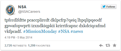
A famous substitution cipher is the Caesar cipher, rotating each letter a number of places.

According to wikipedia, the cipher was reasonably secure at the time because Caesar's enemies would have been illiterate. :-)

The following macro rotates each letter in cell B2 by a number found in cell B8.

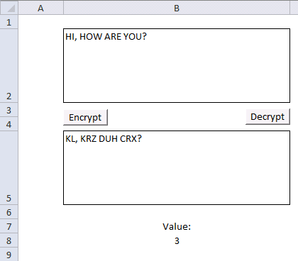
VBA Code

Sub Encrypt()
Dim enc As String
Dim res As String

enc = Range("B2")
For i = 1 To Len(enc)
    If Asc(UCase(Mid(enc, i, 1))) < 91 And Asc(UCase(Mid(enc, i, 1))) > 64 Then
        If (Asc(UCase(Mid(enc, i, 1))) + Range("B8")) > 90 Then
            res = res & Chr(65 + (Asc(UCase(Mid(enc, i, 1))) + Range("B8") - 90))
        ElseIf (Asc(UCase(Mid(enc, i, 1))) + Range("B8")) < 65 Then
            res = res & Chr(90 - (64 - (Asc(UCase(Mid(enc, i, 1))) + Range("B8"))))
        Else
            res = res & Chr(Asc(UCase(Mid(enc, i, 1))) + Range("B8"))
        End If
    Else
        res = res & Mid(enc, i, 1)
    End If
Next i

Range("B5") = res

End Sub

Sub Decrypt()

Dim dec As String
Dim res As String
dec = Range("B5")
For i = 1 To Len(dec)
    If Asc(UCase(Mid(dec, i, 1))) < 91 And Asc(UCase(Mid(dec, i, 1))) > 64 Then
        If (Asc(UCase(Mid(dec, i, 1))) - Range("B8")) > 90 Then
            res = res & Chr(65 + (Asc(UCase(Mid(dec, i, 1))) - Range("B8") - 91))
        ElseIf (Asc(UCase(Mid(dec, i, 1))) - Range("B8")) < 65 Then
            res = res & Chr(90 - (64 - (Asc(UCase(Mid(dec, i, 1))) - Range("B8"))))
        Else
            res = res & Chr(Asc(UCase(Mid(dec, i, 1))) - Range("B8"))
        End If
    Else
        res = res & Mid(dec, i, 1)
    End If
Next i

Range("B2") = res

End Sub

Get excel *.xlsm file

Encrypt message.xlsm

Back to top

12. Transposition cipher

What is a transposition cipher?

A transposition cipher is a way of scrambling the letters in a message so that they appear in a different order. Unlike substitution ciphers, which replace letters with different letters or symbols, a transposition cipher keeps the original letters but rearranges them.

How does the transposition cipher work?

The transposition cipher deploys characters in a grid based on the number of columns entered in cell C3.

Concatenate characters starting from the upper left corner moving down, then continue with the next column, and so on. The formula below adds a | character to show if the last character is the space character.

The transposition cipher can be broken using frequency analysis and anagramming.

Formula in cell C4:

Let's break it down:

1. LEN(C2) returns the length of the text in cell C2. In this example, 16 characters.
2. MOD(LEN(C2), C3) returns the remainder of the division of the length of the text by the value in cell C3.   16/3 = 5,33333 full rows and one character left in the bottom row. The remainder is 1.
3. C3-MOD(LEN(C2), C3) calculates the number of spaces needed to pad the text. This calculates how many containers are empty in the table. 3-1 = 2 containers at the bottom of the table are empty.
4. REPT(" ", ...) repeats the space character to fill empty containers in the table. In this example, 2 space characters.
5. C2&REPT(" ", C3-MOD(LEN(C2), C3)): This part of the formula is padding the text in cell C2 with spaces to make its length a multiple of the value in cell C3. The ampersand & concatenates the original text with the padded spaces.
6. ROUNDUP(LEN(C2)/C3,0) calculates the number of rows needed, rounding up to the nearest whole number.
7. SEQUENCE(..., C3, 1) generates an array of numbers from 1 to the string length in cell C2. It has the same number of columns as specified in cell C3 and rows calculated in step 6.
   
8. MID(..., SEQUENCE(ROUNDUP(LEN(C2)/C3,0), C3, 1), 1): extracts one character from the padded text at each position in the array.
   
9. TRANSPOSE(...): This function transposes the array of characters so rows become columns and columns become rows.
   
10. TEXTJOIN(, FALSE, ...)&"|": This function joins the characters into a single text string, with a "|" delimiter at the end.
    • The first argument , is the delimiter, which is empty in this case, so the characters will be joined without any separator.
    • The second argument FALSE means that the function will ignore empty values.
    • The third argument is the array of characters.
    • &"|" concatenates the "|" delimiter at the end of the joined string.

Step 10 returns "WRNRTKEEDAA AUETC |" which is the encrypted message based on a transposition cipher with 3 columns wide.

The formula in cell C9 decrypts the message and removes the last | character automatically. Change LEN(C7)-1 to Len(C7) to remove that functionality if needed.

Formula in cell C9:

Back to top

13. Columnar transposition cipher

The column transposition cipher uses a key to rearrange the columns in a given order based on the positions of the key characters in the alphabet.

Formula in cell C4:

Let's break it down:

=TEXTJOIN("",FALSE,SORTBY(TRANSPOSE(MID(C2&REPT(" ",MOD(ROUNDUP(LEN(C3&C2)/LEN(C3),0)*LEN(C3),LEN(C2&C3))),SEQUENCE(ROUNDUP(LEN(C2)/LEN(C3),0),LEN(C3)),1)),MID(C3,SEQUENCE(LEN(C3)),1)))

1. LEN(C2) returns the length of the text in cell C2. In this example, "LEMON ORANGE AND APPLES" has 23 characters.
2. ROUNDUP(LEN(C2)/LEN(C3),0) calculates the number of rows needed, rounding up to the nearest whole number. 23/4 = 5.75 which returns 6.
3. SEQUENCE(ROUNDUP(LEN(C2)/LEN(C3), 0), LEN(C3)) generates an array of numbers from 1 to the string length in cell C2. It has the same number of columns as specified in cell C3 and rows calculated in step 2 above.
   
4. C2&REPT(" ",MOD(ROUNDUP(LEN(C3&C2)/LEN(C3),0)*LEN(C3),LEN(C2&C3))): Pads the string in cell C2 with needed space characters to fill the entire table.
5. MID(C2, ... , LEN(C3)), 1): extracts one character from the text in cell C2 at each position in the array.
   
6. TRANSPOSE(...): This function transposes the array of characters so rows become columns and columns become rows.
   
7. SORTBY(..., MID(C3, SEQUENCE(LEN(C3)), 1)): Sorts the rows (which were columns before step 5) based on the specified key in cell C3 which in this example is "PEAR"
   
   The following image shows the columns being sorted based on key "PEAR", however, the arrays are transposed and not in this layout shown below.
   
   
8. TEXTJOIN(, FALSE, ...)&"|": This function joins the characters into a single text string, with a "|" delimiter at the end.
   • The first argument , is the delimiter, which is empty in this case, so the characters will be joined without any separator.
   • The second argument FALSE means that the function will ignore empty values.
   • The third argument is the array of characters.
   • &"|" concatenates the "|" delimiter at the end of the joined string.
9. LET(z,LEN(C3&C2),y,LEN(C3),x,ROUNDUP(z/y,0), ... ): The LET function lets you assign variables to intermediate calculations, this may shorten the formula considerably.

Step 8 concatenates all characters row by row creating this string: "MOGNPSE NAAELNA LOREDP"

The formula in cell C8 decrypts the cipher string in cell C6:

Back to top

14. Double columnar transposition cipher

The double columnar transposition cipher uses two keys instead of one, see section 13 above. In other words, this is simply a columnar transposition applied twice.

This cipher is one of the most secure classic ciphers and was used successfully by both the allies and axis during the second world war. The image above shows only one key, the double columnar transposition cipher uses two keys. This can be done by performing the encryption twice, each time with a different key.

Back to top

15. Vigenere cipher

The Vigenere cipher uses the same key repeatedly across the entire message, here are links to detailed explanations:

• Vigenere cipher
• What is Vigenere Cipher?

The formulas finds the relative position of each character of both plain text message and the code key in the alphabet, provided in cell B10.

They then add the numbers, see image above. The sum is then the position of a different character in the alphabet.

Sometimes the sum is larger than the number of characters in the provided alphabet. The formulas calculate the remainder and use that number to extract a character.

You can change the alphabet in cell B10 to only upper letters if you want a more read-friendly code. Also, replace the FIND function with the SEARCH function in the formulas below or make sure that you only use upper letters in cell C2.

The formula in cell C4 returns an error if a character is not found in cell B10.

Formula in cell C4:

Formula in cell C8:

Explaining formula in cell C4

Step 1 - Count characters

The LEN function returns the number of characters in a cell value.

Function syntax: LEN(text)

LEN(C2) returns 15.

Step 2 - Create an array of numbers from 1 to n horizontally

The SEQUENCE function creates a list of sequential numbers.

Function syntax: SEQUENCE(rows, [columns], [start], [step])

SEQUENCE(,LEN(C2)) returns {1,2,3,... ,15}

Step 3 - Split characters in cell C2

The MID function returns a substring from a string based on the starting position and the number of characters you want to extract.

Function syntax: MID(text, start_num, num_chars)

MID(C2,SEQUENCE(,LEN(C2)),1) returns {"D","E","F","E","N","D","T","H","E","C","A","S","T","L","E"}

Step 4 - Calculate position in alphabet for plain text

The FIND function returns the position of a specific string in another string, reading left to right. Note, the FIND function is case-sensitive.

Function syntax: FIND(find_text,within_text, [start_num])

FIND(MID(C2,SEQUENCE(,LEN(C2)),1),$B$10)-1 returns {3,4,5,... ,4}

Step 5 - Create a repeating sequence

The MOD function returns the remainder after a number is divided by divisor.

Function syntax: MOD(number, divisor)

MOD(SEQUENCE(,LEN(C2))-1, LEN(C3)) returns {0,1,2,3,4,5,6,7,8,9,0,1,2,3,4}

Step 6 - Split characters in code key

The MID function returns a substring from a string based on the starting position and the number of characters you want to extract.

Function syntax: MID(text, start_num, num_chars)

MID(C3,MOD(SEQUENCE(,LEN(C2))-1,LEN(C3))+1,1) returns {"K","I","N","G","A","R","T","H","U","R","K","I","N","G","A"}

Step 7 - Find relative position in alphabet for each character in code key

The FIND function returns the position of a specific string in another string, reading left to right. Note, the FIND function is case-sensitive.

Function syntax: FIND(find_text,within_text, [start_num])

FIND(MID(C3, MOD(SEQUENCE(,LEN(C2))-1, LEN(C3))+1, 1), B10) returns {11,9,14,... ,1}

Step 8 - Add arrays and subtract 1

The plus and minus signs let you add and subtract numbers respectively in an Excel formula.

FIND(MID(C2, SEQUENCE(,LEN(C2)), 1), B10)-1+FIND(MID(C3, MOD(SEQUENCE(,LEN(C2))-1

returns {14,13, ... ,5}

Step 9 - Calculate the remainder

The MOD function returns the remainder after a number is divided by divisor.

Function syntax: MOD(number, divisor)

MOD(FIND(MID(C2,SEQUENCE(,LEN(C2)),1),$B$10)-1+FIND(MID(C3,MOD(SEQUENCE(,LEN(C2))-1,LEN(C3))+1,1),$B$10),LEN(B10))

returns {14,13,19,... ,5}

Step 10 - Get characters

The MID function returns a substring from a string based on the starting position and the number of characters you want to extract.

Function syntax: MID(text, start_num, num_chars)

MID(B10, MOD(FIND(MID(C2, SEQUENCE(LEN(C2)), 1), B10)-1+FIND(MID(C3, MOD(SEQUENCE(LEN(C2))-1, LEN(C3))+1, 1), B10), LEN(B10))+1, 1) returns {"N","M","S",...,"E"}

Step 11 - Join letters

The TEXTJOIN function combines text strings from multiple cell ranges.

Function syntax: TEXTJOIN(delimiter, ignore_empty, text1, [text2], ...)

TEXTJOIN(, TRUE, MID(B10, MOD(FIND(MID(C2, SEQUENCE(LEN(C2)), 1), B10)-1+FIND(MID(C3, MOD(SEQUENCE(LEN(C2))-1, LEN(C3))+1, 1), B10), LEN(B10))+1, 1))

returns "NMSKNUMOYTKAGRE".

Back to top

16. Running key cipher

The running key cipher is a Vigenere cipher with a longer key from a book. The formulas below and above are the same, only the key is different.

The running key cipher is explained here: Running key

Formula in cell C4:

Formula in cell C8:

Back to top

17. One-Time Pad cipher

The One-Time Pad cipher works just like the Vigenere cipher, however, the key must be random and not pseudo-random. It is not possible to crack a One-Time Pad cipher in theory, as long as the keys are only used once hence the name One-Time.

The One-Time Pad cipher is explained here: One-Time Pad

Formula in cell C4:

Formula in cell C7:

Back to top

18. Autokey cipher

The Autokey cipher is a Vigenere cipher, however, it uses the plaintext message concatenated with the real key. I have not yet figured out how to build a formula that can decrypt an Autokey cipher.

The LAMBDA function seems interesting, you can create a recursive function which seems handy in this case. It is still only available for Office Insiders.

Formula in cell C4:

Formula in cell C4:

Back to top

19. Homophonic substitution cipher (1)

The homophonic substitution cipher maps each character to a different character just like the simple substitution cipher, however, some characters are mapped to multiple characters which makes the cipher harder to break using frequency analysis.

I am using the following table to map characters, the formula picks a character randomly if more than one is entered.

Formula in cell B3:

Formula in cell B7:

20. Homophonic substitution cipher (2)

This example is also a homophonic substitution cipher, however, a much larger table is used. It contains three unique digits per cell.

Formula in cell B3:

Formula in cell B7:

Back to top

21. XOR

The formula in cell C3 converts each character to ASCII code and then performs bitwise XOR between the code key and the ASCII code.

Formula in cell C3:

Formula in cell C7:

Back to top

22. Four-square cipher

The four-square cipher is a classic cipher from the 19 century that uses four grids to encrypt and decrypt messages. Two different code keys are used to change two of the grids.

The two first characters in the plain text are "a" and "m", find character "a" in the upper left grid, and find the character "m" in the lower right grid. They form a rectangle across all four grids, the two other characters in the opposite corners of the rectangle are the encrypted characters.

Note that the first code key is in the upper-right grid and the second code key is in the lower-left grid. The formulas below calculate the corresponding characters based on the plain text entered in cell C2.

Formula in cell C5:

Formula in cell C10:

Back to top

23. Straddling checkerboard

The Straddling checkerboard converts letters to digits based on the table shown in the image below.

The table contains numbers distributed above and to the left of a secret alphabet. For example, character "s" is in column 9 and the first row, the first row has no name (blank). The encrypted number for character "s" is 9.

Character "u" is in column 3 and row 6 the encrypted numbers for character "u" is therefore 63.

The straddling checkerboard is broken with frequency analysis.

Formula in cell C5:

Formula in cell C10:

Back to top

24. ADFGVX cipher

The ADFGVX cipher converts each character to two different characters based on a grid, see image below.

A secret alphabet is used, see image above. The formulas below use the text string in cell F2, change this text string to create your own secret alphabet. Note that character "J" is not in the grid, if you have one in your plain text replace that character with I.

Formula in cell C3:

Replace array below {"A", "B", "C", "D", "E";"F", "G", "H", "IJ", "K";"L", "M", "N", "O", "P";"Q", "R", "S", "T", "U";"V", "W", "X", "Y", "Z"} with your secret alphabet. The order is important to successfully encrypt and decrypt messages.

Formula in cell C10:

Back to top

25. Polybius square

The Polybius square encrypts a message by placing each character in a grid. The encrypted text is the column and row number of each character concatenated to a long string.

Formula in cell C3:

Formula in cell C10:

26. Nihilist cipher

Formula in cell C3:

Formula in cell C10:

Back to top

27. Bifid cipher

Formula in cell C3:

Formula in cell C6:

Back to top

28. Trifid

Back to top

29. Frequency analysis

Formula in cell C6:

Formula in cell D6:

Back to top

30. Tabula recta

Formula in cell C5:

Back to top

31. Insert random characters based on a key - LAMBDA function

This formula pads a text string with random letters based on a a given key. The key specifies how many random letters are between each letter in the text string.

Excel 365 formula in cell C4:

Explaining formula

The key "CAD" specifies the number of random characters between each letter in the text string. "C" is the third letter in the alphabet, three random letters are attached to the first letter in the text string. In this example letters "SNL" to "F".

The second letter in the key is "A", it is the first letter in the alphabet, one random letter is needed between the first and second letters in the text string. "SNLF" and "R" becomes "SNLFR".

The third letter in the key is "D", it is the fourth letter in the alphabet. The formula appends four random letters between the second and third letters in the text string. The key is repeated until all characters are padded with random letters.

Step 1 - Count characters in the given text string

The LEN function returns the number of characters in a cell value.

Function syntax: LEN(text)

LEN(C2) returns 11.

Step 2 - Divide character lengths for text and key strings

The division sign lets you divide numbers in an Excel formula.

LEN(C2)/LEN(C3) returns 3.6666666667

Step 3 - Round the number up to its nearest integer

The ROUNDUP function calculates a number rounded up based on the number of digits to which you want to round the number.

Function syntax: ROUNDUP(number, num_digits)

ROUNDUP(LEN(C2)/LEN(C3),0) returns 4.

Step 4 - Repeat key string

The REPT function repeats a specific text a chosen number of times.

Function syntax: REPT(text,number_times)

REPT(C3,ROUNDUP(LEN(C2)/LEN(C3),0)) returns "CADCADCADCAD"

Step 7 - Extract n characters from left

The LEFT function extracts a specific number of characters always starting from the left.

Function syntax: LEFT(text, [num_chars])

LEFT(REPT(C3,ROUNDUP(LEN(C2)/LEN(C3),0)),LEN(C2)) returns "CADCADCADCA".

Step 8 -

The SEQUENCE function creates a list of sequential numbers.

Function syntax: SEQUENCE(rows, [columns], [start], [step])

SEQUENCE(LEN(C2))

Step 9 -

The MID function returns a substring from a string based on the starting position and the number of characters you want to extract.

Function syntax: MID(text, start_num, num_chars)

MID(LEFT(REPT(C3,ROUNDUP(LEN(C2)/LEN(C3),0)),LEN(C2)),SEQUENCE(LEN(C2)),1)

Step 10 -

The SEARCH function returns the number of the character at which a specific character or text string is found reading left to right (not case-sensitive)

Function syntax: SEARCH(find_text,within_text, [start_num])

SEARCH(MID(LEFT(REPT(C3,ROUNDUP(LEN(C2)/LEN(C3),0)),LEN(C2)),SEQUENCE(LEN(C2)),1),"ABCDEFGHIJKLMNOPQRSTUVWXYZ")

Step 11 -

The RANDARRAY function creates an array of random numbers

Function syntax: RANDARRAY([rows], [columns], [min], [max], [whole_number])

RANDARRAY(,b,65,90,1)

Step 12 -

The VSTACK function combines cell ranges or arrays. Joins data to the first blank cell at the bottom of a cell range or array (vertical stacking)

Function syntax: VSTACK(array1,[array2],...)

VSTACK(a,RANDARRAY(,b,65,90,1))

Step 13 -

The LAMBDA function build custom functions without VBA, macros or javascript.

Function syntax: LAMBDA([parameter1, parameter2, …,] calculation)

LAMBDA(a,b,VSTACK(a,RANDARRAY(,b,65,90,1)))

Step 14 -

The REDUCE function shrinks an array to an accumulated value, a LAMBDA function is needed to properly accumulate each value in order to return a total.

Function syntax: REDUCE([initial_value], array, lambda(accumulator, value))

REDUCE("",SEARCH(MID(LEFT(REPT(C3,ROUNDUP(LEN(C2)/LEN(C3),0)),LEN(C2)),SEQUENCE(LEN(C2)),1),"ABCDEFGHIJKLMNOPQRSTUVWXYZ"),LAMBDA(a,b,VSTACK(a,RANDARRAY(,b,65,90,1))))

Step 15 -

The CHAR function converts a number to the corresponding ANSI character determined by your computers character set.

Function syntax: CHAR(text)

CHAR(REDUCE("",SEARCH(MID(LEFT(REPT(C3,ROUNDUP(LEN(C2)/LEN(C3),0)),LEN(C2)),SEQUENCE(LEN(C2)),1),"ABCDEFGHIJKLMNOPQRSTUVWXYZ"),LAMBDA(a,b,VSTACK(a,RANDARRAY(,b,65,90,1)))))

Step 16 -

The DROP function removes a given number of rows or columns from a 2D cell range or array.

Function syntax: DROP(array, rows, [columns])

DROP(CHAR(REDUCE("",SEARCH(MID(LEFT(REPT(C3,ROUNDUP(LEN(C2)/LEN(C3),0)),LEN(C2)),SEQUENCE(LEN(C2)),1),"ABCDEFGHIJKLMNOPQRSTUVWXYZ"),LAMBDA(a,b,VSTACK(a,RANDARRAY(,b,65,90,1))))),1)

Step 17 -

The IFERROR function if the value argument returns an error, the value_if_error argument is used. If the value argument does NOT return an error, the IFERROR function returns the value argument.

Function syntax: IFERROR(value, value_if_error)

IFERROR(DROP(CHAR(REDUCE("",SEARCH(MID(LEFT(REPT(C3,ROUNDUP(LEN(C2)/LEN(C3),0)),LEN(C2)),SEQUENCE(LEN(C2)),1),"ABCDEFGHIJKLMNOPQRSTUVWXYZ"),LAMBDA(a,b,VSTACK(a,RANDARRAY(,b,65,90,1))))),1),"")

Step 18 -

MID(C2,SEQUENCE(LEN(C2)),1)

Step 19 -

The HSTACK function combines cell ranges or arrays. Joins data to the first blank cell to the right of a cell range or array (horizontal stacking)

Function syntax: HSTACK(array1,[array2],...)

HSTACK(IFERROR(DROP(CHAR(REDUCE("",SEARCH(MID(LEFT(REPT(C3,ROUNDUP(LEN(C2)/LEN(C3),0)),LEN(C2)),SEQUENCE(LEN(C2)),1),"ABCDEFGHIJKLMNOPQRSTUVWXYZ"),LAMBDA(a,b,VSTACK(a,RANDARRAY(,b,65,90,1))))),1),""),MID(C2,SEQUENCE(LEN(C2)),1))

Step 20 -

The TEXTJOIN function combines text strings from multiple cell ranges.

Function syntax: TEXTJOIN(delimiter, ignore_empty, text1, [text2], ...)

TEXTJOIN("",1,HSTACK(IFERROR(DROP(CHAR(REDUCE("",SEARCH(MID(LEFT(REPT(C3,ROUNDUP(LEN(C2)/LEN(C3),0)),LEN(C2)),SEQUENCE(LEN(C2)),1),"ABCDEFGHIJKLMNOPQRSTUVWXYZ"),LAMBDA(a,b,VSTACK(a,RANDARRAY(,b,65,90,1))))),1),""),MID(C2,SEQUENCE(LEN(C2)),1)))

Excel 365 formula in cell C8:

Back to top

Get the Excel file

Working-with-ciphers.xlsx

Excel categories

Comments (14)