How to return a value if lookup value is in a range
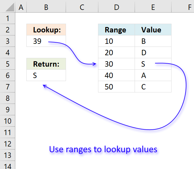
In this article, I will demonstrate four different formulas that allow you to lookup a value that is to be found in a given range and return the corresponding value on the same row. If you need to return multiple values because the ranges overlap then read this article: Return multiple values if in range.
What's on this page
- If value in range then return value - LOOKUP function
- If value in range then return value - INDEX + SUMPRODUCT + ROW
- If value in range then return value - VLOOKUP function
- If value in range then return value - INDEX + MATCH
- Match a range value containing both text and numerical characters
- Return multiple values if in range
- Create numbers based on numerical ranges - Excel 365
- Create numbers based on numerical ranges - earlier Excel versions
- Distribute values across numerical ranges
They all have their pros and cons and I will discuss those in great detail, they can be applied to not only numerical ranges but also text ranges and date ranges as well.
I have made a video that explains the LOOKUP function in context to this article, if you are interested.
There is a file for you to get, at the end of this article, which contains all the formula examples in a worksheet each.
You can use the techniques described in this article to calculate discount percentages based on price intervals or linear results based on the lookup value.
The following table shows the differences between the formulas presented in this article.
| Formula | Range sorted? | Array formula | Get value from any column? | Two range columns? |
| LOOKUP | Yes | No | Yes | No |
| INDEX + SUMPRODUCT + ROW | No | No | Yes | Yes |
| VLOOKUP | Yes | No | No | No |
| INDEX + MATCH | Yes | No | Yes | No |
Some formulas require you to have the lookup range sorted to function properly, the INDEX+SUMPRODUCT+ROW alternative is the only way to go if you can't sort the values.
The disadvantage with the INDEX+SUMPRODUCT+ROW formula is that you need start and end values, the other formulas use the start values also as end range values.
The VLOOKUP function can only search the leftmost column, you must rearrange your table to meet this condition if you are going to use the VLOOKUP function.
1. If value in range then return value - LOOKUP function
To better demonstrate the LOOKUP function I am going to answer the following question.
Hi,
What type of formula could be used if you weren't using a date range and your data was not concatenated?
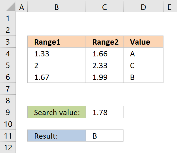
ie: Input Value 1.78 should return a Value of B as it is between the values in Range1 and Range2
Range1 Range2 Value
1.33 1.66 A
1.67 1.99 B
2.00 2.33 C
The next image shows the table in greater detail.
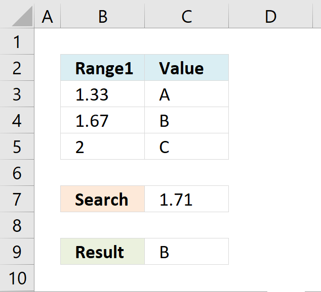
The picture above shows data in cell range B3:C5, the search value is in C7 and the result is in C9.
Cell range B3:B5 must be sorted in ascending order for the LOOKUP function to work properly.
If an exact match is not found the largest value is returned as long as it is smaller than the lookup value.
The LOOKUP function then returns a value in a column on the same row.
The formula in cell C9:
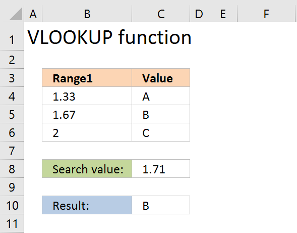
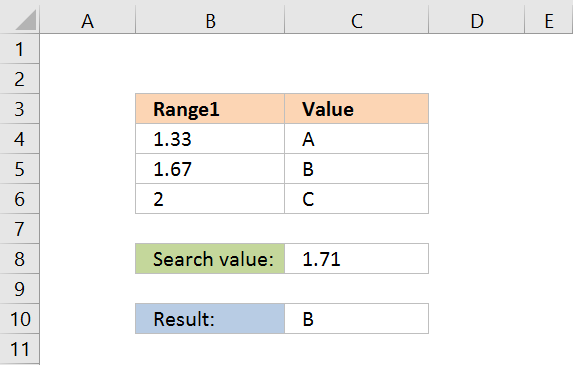
Example, Search value 1.71 has no exact match, the largest value that is smaller than 1.71 is 1.67. The returning value is found in column C on the same row as 1.67, in this case, B.
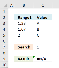 If the search value is smaller than the smallest value in the lookup range the function returns #N/A meaning Not Available or does not exist.
Example in the picture to the right, search value is 1 in the and the LOOKUP function returns #N/A.
To solve this problem simply add another number, for example 0. Cell range B3:B6 would then contain 0, 1.33, 1.67, 2.
A search value greater than the largest value in the lookup range matches the largest value. Example in above picture, search value is 3 and the returning value is C.
Watch video below to see how the LOOKUP function works:
Learn more about the LOOKUP function, recommended reading:
Recommended articles
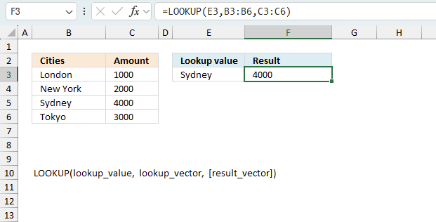
Finds a value in a sorted cell range and returns a value on the same row.
Tip! - You can quickly sort a cell range, follow these steps:
- Press with right mouse button on on a cell in the cell range you want to sort
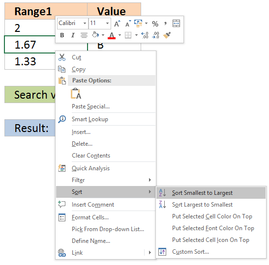
- Hover with mouse cursor over Sort
- Press with mouse on "Sort Smallest to Largest"
2. If the value is in the range then return value - INDEX + SUMPRODUCT + ROW
The following formula is slightly larger but you don't need to sort cell range B4:B6.
The formula in cell C11:
The ranges don't need to be sorted however you need a start (Range1) and an end value (Range2).
Explaining formula in cell C11
You can easily follow along, go to tab "Formulas" and press with left mouse button on "Evaluate Formula" button. Press with left mouse button on "Evaluate" button to move to next step.
Step 1 - Calculate first condition
The bolded part is the the logical expression I am going to explain in this step.
=INDEX(D4:D6, SUMPRODUCT(--($D$8<=C4:C6), --($D$8>=B4:B6), ROW(A1:A3)))
Logical operators
= equal sign
> less than sign
< greater than sign
The greater than sign combined with the equal sign <= means if value in cell D8 is smaller than or equal to the values in cell range C4:C6.
returns {0;1;1}.
The double minus signs convert the boolean value TRUE or FALSE to the corresponding number 1 or 0 (zero).
Step 2 - Calculate second criterion
=INDEX(D4:D6, SUMPRODUCT(--($D$8<=C4:C6), --($D$8>=B4:B6), ROW(A1:A3)))
returns {1;1;0}
Step 3 - Create row numbers
=INDEX(D4:D6, SUMPRODUCT(--($D$8<=C4:C6), --($D$8>=B4:B6), ROW(A1:A3)))
ROW(A1:A3) returns {1;2;3}
Step 4 - Multiply criteria and row numbers and sum values
=INDEX(D4:D6, SUMPRODUCT(--($D$8<=C4:C6), --($D$8>=B4:B6), ROW(A1:A3)))
SUMPRODUCT(--($D$8<=C4:C6), --($D$8>=B4:B6), ROW(A1:A3))
returns number 2.
Step 5 - Return a value of the cell at the intersection of a particular row and column
=INDEX(D4:D6, SUMPRODUCT(--($D$8<=C4:C6), --($D$8>=B4:B6), ROW(A1:A3)))
returns "B".
Functions in this formula: INDEX, SUMPRODUCT, ROW
3. If value in range then return value - VLOOKUP function
The VLOOKUP function requires the table to be sorted based on range1 in an ascending order.
Explaining the VLOOKUP formula in cell C10
The VLOOKUP function looks for a value in the leftmost column of a table and then returns a value in the same row from a column you specify.
VLOOKUP(
lookup_value,
table_array,
col_index_num, [range_lookup]
)
The [range_lookup] argument is important in this case, it determines how the VLOOKUP function matches the lookup_value in the table_array.
The [range_lookup] is optional, it is either TRUE (default) or FALSE. It must be TRUE in our example here so that VLOOKUP returns an approximate match.
In order to do an approximate match the table_array must be sorted in an ascending order based on the first column.
=VLOOKUP($D$8,$B$4:$D$6,3,TRUE)
becomes
=VLOOKUP(1,78,{1,33, 1,66, "A";1,67, 1,99, "B";2, 2,33, "C"},3,TRUE)
1,67 is the next largest value and the VLOOKUP function returns "B".
4. If value in range then return value - INDEX + MATCH
Formula in cell C10:
The lookup range must be sorted, just like the LOOKUP and VLOOKUP functions. Functions in this formula: INDEX and MATCH
Thanks JP!
Explaining INDEX+MATCH in cell D10
=INDEX($D$4:$D$6,MATCH(D8,$B$4:$B$6,1))
Step 1 - Return the relative position of an item in an array
The MATCH function returns the relative position of an item in an array or cell range that matches a specified value
MATCH(
lookup_value,
lookup_array,
[match_type])
)
The [match_type] argument is optional. It can be either -1, 0, or 1. 1 is default value if omitted.
The match_type argument determines how the MATCH function matches the lookup_value with values in lookup_array.
We want it to do an approximate search so I am going to use 1 as the argument.
This will make the MATCH find the largest value that is less than or equal to lookup_value. However, the values in the lookup_array argument must be sorted in an ascending order.
To learn more about the [match_type] argument read the article about the MATCH function.
=INDEX($D$4:$D$6,MATCH(D8,$B$4:$B$6,1))
MATCH(D8,$B$4:$B$6,1)
becomes
MATCH(1.78,{1.33;1.67;2},1)
1.67 is the largest value that is less than or equal to lookup_value. 1.67 is the second value in the array. MATCH function returns 2.
Step 2 - Return a value of the cell at the intersection of a particular row and column
=INDEX($D$4:$D$6,MATCH(D8,$B$4:$B$6,1))
returns "B".
5. Match a range value containing both text and numerical characters
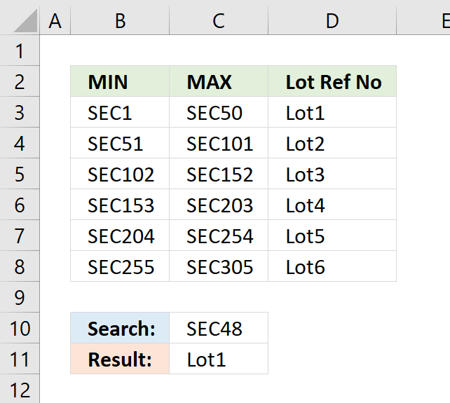
This section demonstrates how to match a value containing both text and digits to ranges. The search value is specified in cell C10, cell range B3:B8 contains the start values for the ranges and C3:C8 contains the end values for the ranges.
The formula matches the numerical part of the value in cell C10 to the start and end numbers for each range, it returns a corresponding value from cell range D3:D8.
For example, cell C10 contains SEC48. The numerical part is 48, 48 is larger than the numerical part in cell B3 and lower than C3. The corresponding value from D3:D8 is cell D3 which is returned to cell C11.
Array formula in cell C11:
How to enter an array formula
Excel 365 users can ignore the following steps.
This formula is an array formula. To enter an array formula, type the formula in a cell then press and hold CTRL + SHIFT simultaneously, now press Enter once. Release all keys.
The formula bar now shows the formula with a beginning and ending curly bracket telling you that you entered the formula successfully. Don't enter the curly brackets yourself.
Explaining formula in cell C11
Step 1 - Extract number from search value
The MID function returns a given number of characters from a value. This allows us to extract only the numbers from the value.
MID(C10,4,999)
returns "48".
This is still a text value so in order to use that, we must first convert it to a numerical value.
MID(C10,4,999)*1
returns 48.
Step 2 - Extract numbers from lookup range
The second argument in the LOOKUP function is the lookup list. This list must also be converted into numbers. I will use the same technique described in the previous step to extract and convert the numbers from cell range B3:B8.
MID(B3:B8,4,999)*1
returns {1;51;102;153;204;255}.
Step 3 - Return corresponding value on the same row as the matching value
The LOOKUP function matches the lookup value to a list of range values and returns the corresponding value. Remember that the list of values must be sorted in an ascending order for it to work.
LOOKUP(MID(C10,4,999)*1,MID(B3:B8,4,999)*1,D3:D8)
returns "Lot1" in cell C11.
Get Excel *.xlsx file
Match text and numbers combined.xlsx
Alternative formula
Back to top
Quickly lookup a value in a numerical range
You can also do lookups in date ranges, dates in Excel are actually numbers.
6. Return multiple values if in range
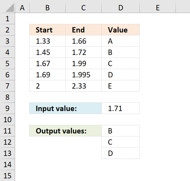
The image above shows a formula in cell C11 that extracts values from column D if the number in cell D9 is in a range specified in B3:B7 and C3:C7. This formula extracts multiple values if multiple ranges match.
The example above extracts B, C and D because 1.71 is between 1.45 - 1.72 (B), 1.67-1.99 (C) and 1.69-1.995 (D).
Array formula in cell C11:
Explaining formula in cell C11
Step 1 - Check if number is larger than or equal to numbers in column B
The less than sign and the equal sign compares the numbers, if a number in column B is smaller than or equal to number in cell D9 then it evaluates to TRUE, if not FALSE.
$B$3:$B$7<=$D$9
returns {TRUE; TRUE; TRUE; TRUE; FALSE}.
Step 2 - Check if number is smaller than or equal to numbers in column C
$C$3:$C$7>=$D$9
returns {FALSE; TRUE; TRUE; TRUE; TRUE}
Step 3 - AND logic
Now we multiply the arrays, both logical expression must evaluate to TRUE in order to get the correct value(s). The parentheses are there to make sure that the correct calculation order is maintained.
($B$3:$B$7<=$D$9)*($C$3:$C$7>=$D$9)
returns {0;1;1;1;0}.
Step 4 - Replace TRUE with row number
The IF function returns a unique number if boolean value is TRUE. FALSE returns "" (nothing).
IF(($B$3:$B$7<=$D$9)*($C$3:$C$7>=$D$9), MATCH(ROW($D$3:$D$7), ROW($D$3:$D$7)), "")
returns {"";2;3;4;""}.
Step 5 - Extract k-th smallest row number
The SMALL function lets you calculate the k-th smallest value from a cell range or array. SMALL( array, k)
SMALL(IF(($B$3:$B$7<=$D$9)*($C$3:$C$7>=$D$9), MATCH(ROW($D$3:$D$7), ROW($D$3:$D$7)), ""), ROWS($A$1:A1))
returns 2.
Step 6 - Get corresponding value
The INDEX function returns a value based on row number (and column number if needed)
INDEX($D$3:$D$7, SMALL(IF(($B$3:$B$7<=$D$9)*($C$3:$C$7>=$D$9), MATCH(ROW($D$3:$D$7), ROW($D$3:$D$7)), ""), ROWS($A$1:A1)))
returns "B" in cell C11.
Get Excel *.xlsx file
Return multiple values if in range.xlsx
7. Create numbers based on numerical ranges - Excel 365
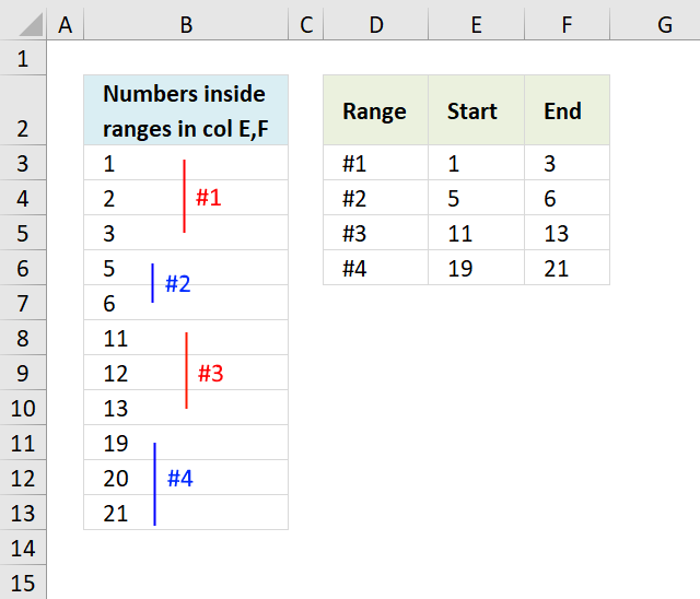
The image above demonstrates a formula in cell B3 that lists numbers from 1 to 21 only if they meet the numerical ranges specified in cell range E3:F6.
The first numerical range is 1 to 3, the second is 5 to 6, the third is 11 to 13, and the last one is 19 to 21. The numbers that meet these criteria are listed in cell B3 and cells below as far as needed. They are 1, 2, 3, 5, 6, 11, 12, 13, 19, 20, and 21. The numbers that don't meet the criteria in cell range E3:F6 are 4, 7, 8, 9, 10, 14, 15, 16, 17, and 18.
Excel 365 dynamic array formula in cell B3:
1.2 Explaining the formula
Step 1 - Build an array containing numbers from 1 to 21
The ROW function calculates the row number of a cell reference.
Function syntax: ROW(reference)
ROW(A1:A21)
returns
{1; 2; ... ; 21}
Step 2 - Check numbers that meet criteria
The COUNTIFS function calculates the number of cells across multiple ranges that equals all given conditions.
Function syntax: COUNTIFS(criteria_range1, criteria1, [criteria_range2, criteria2]…)
COUNTIFS($E$3:$E$6, "<="&ROW(A1:A21),$F$3:$F$6, ">="&ROW(A1:A21))
becomes
COUNTIFS({1;5;11;19}, "<="&{1; 2; ... ; 21},{3;6;13;21}, ">="&{1; 2; ... ; 21})
and returns
{1; 1; 1; 0; 1; 1; 0; 0; 0; 0; 1; 1; 1; 0; 0; 0; 0; 0; 1; 1; 1}
Step 3 - Filter numbers based on array
The FILTER function extracts values/rows based on a condition or criteria.
Function syntax: FILTER(array, include, [if_empty])
FILTER(ROW(A1:A21),COUNTIFS($E$3:$E$6, "<="&ROW(A1:A21),$F$3:$F$6, ">="&ROW(A1:A21)))
returns {1; 2; 3; 5; 6; 11; 12; 13; 19; 20; 21}
Step 4 - Shorten formula
The LET function lets you name intermediate calculation results which can shorten formulas considerably and improve performance.
Function syntax: LET(name1, name_value1, calculation_or_name2, [name_value2, calculation_or_name3...])
ROW(A1:A21) is repeated three times in the formula.
FILTER(ROW(A1:A21),COUNTIFS($E$3:$E$6, "<="&ROW(A1:A21),$F$3:$F$6, ">="&ROW(A1:A21)))
x - ROW(A1:A21)
LET(x,ROW(A1:A21),FILTER(x,COUNTIFS($E$3:$E$6, "<="&x,$F$3:$F$6, ">="&x)))
8. Create numbers based on numerical ranges - earlier Excel versions
The image above shows an array formula in cell B3 that calculates numbers based on the numerical ranges in cell range E3:F6.
Array formula in B3:
To enter an array formula, type the formula in a cell then press and hold CTRL + SHIFT simultaneously, now press Enter once. Release all keys.
The formula bar now shows the formula with a beginning and ending curly bracket telling you that you entered the formula successfully. Don't enter the curly brackets yourself.
Explaining formula in cell B3
Step 1 - Create a sequence
The ROW function returns a row number based on a cell reference, if the cell reference has multiple rows then the row function returns an array of numbers.
ROW($1:$21)
returns
{1; 2; 3; 4; 5; 6; 7; 8; 9; 10; 11; 12; 13; 14; 15; 16; 17; 18; 19; 20; 21}
Step 2 - Check if number is in sequence
The COUNTIFS function checks if a number is larger or equal to the start value and smaller or equal to the end value. If both conditions are met the COUNTIFS function returns 1.
COUNTIFS($E$3:$E$6, "<="&ROW($1:$21),$F$3:$F$6, ">="&ROW($1:$21))
returns {1; 1; 1; 0; 1; 1; 0; 0; 0; 0; 1; 1; 1; 0; 0; 0; 0; 0; 1; 1; 1}
Tip! Use an Excel defined Table to create dynamic cell references that you don't have to adjust if more ranges are added or deleted.
Step 3 - Return number if in range
The IF function has three arguments, the first one must be a logical expression. If the expression evaluates to TRUE then one thing happens (argument 2) and if FALSE another thing happens (argument 3).
IF(COUNTIFS($E$3:$E$6, "<="&ROW($1:$21),$F$3:$F$6, ">="&ROW($1:$21)), ROW($1:$21))
returns {1; 2; 3; FALSE; 5; 6; FALSE; FALSE; FALSE; FALSE; 11; 12; 13; FALSE; FALSE; FALSE; FALSE; FALSE; 19; 20; 21}.
Step 4 - Extract k-th smallest number
The ROWS function keeps track of the numbers based on an expanding cell reference. It will expand as the formula is copied to the cells below.
SMALL(IF(COUNTIFS($E$3:$E$6, "<="&ROW($1:$21),$F$3:$F$6, ">="&ROW($1:$21)), ROW($1:$21)), ROWS($A$1:A1))
becomes SMALL({1; 2; ... ; 21}, 1) and returns 1 in cell B3.
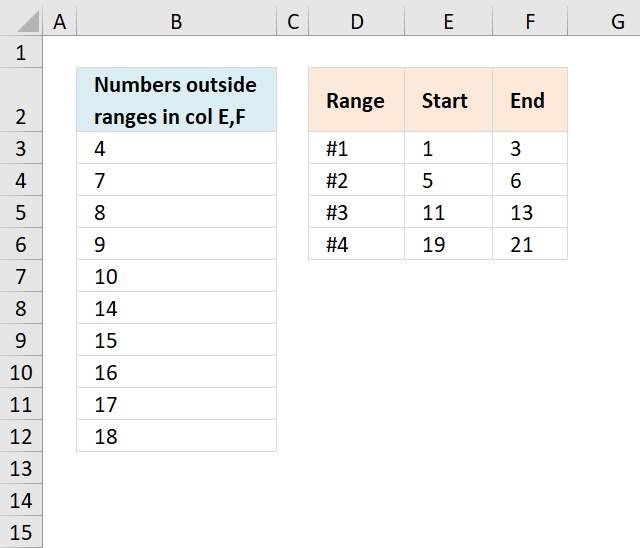
The array formula in cell B3 lists numbers not in ranges specified in cell range E3:F6.
Array formula in B3:
9. Distribute values across numerical ranges
This article demonstrates how to distribute values into specific ranges with possible overlapping ranges. I have written articles about filter rows based on a range criteria and extract records between two dates if you are interested in how to perform lookups based on ranges.
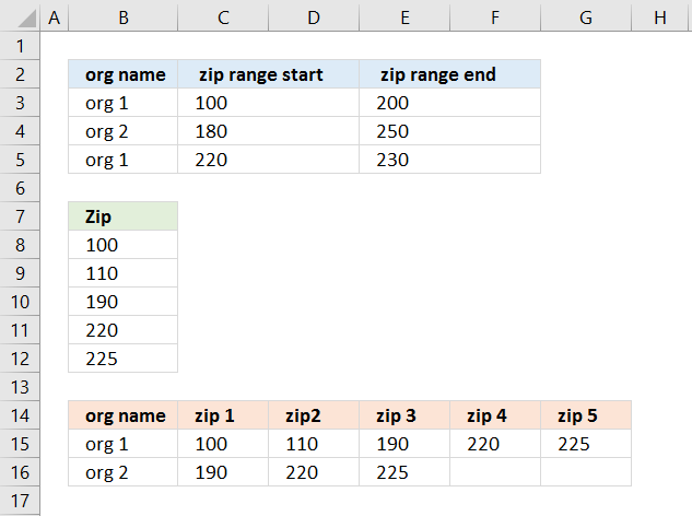
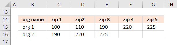
This example, demonstrated in the image above, shows ranges defined in cell B2:F5, note that range "org2" 180-250 partially overlaps "org1" 100-200 and 220-230.
Example values are in cell range B8:B12, they are 100, 110, 190, 220, and 225.
There are two formulas, the first one creates a unique distinct list in cell B15 and cells below. The second formula distributes values across ranges based on item names on the same row in column B, a value may exist in two or more ranges simultaneously.
Value 100 is only in item name "org 1", however, value 190 is in both "org 1" and "org 2". Value 190 matches both range 100-200 and 180-250.
9.1. Question
Thank you *so* much for your detailed examples and for actively replying to users! I have a problem, which I've tried solving by editing your formula examples for 20+ hours without success although I thought I could do it myself but apparently not, so here goes:I have a long list of organizations that work in specific zip areas defined by zip ranges (start and end). One org might have multiple zip ranges and there can be overlap between organizations (i.e. one zip might "belong" to >1 org). Then there's another list that has got all the possible existing zips. I would need to have all existing zips falling inside the zip range of the organization added to separate columns on the matching row of the first list.First list:
org name | zip range start | zip range end
org 1 | 00100 | 00200
org 2 | 00180 | 00250
org 1 | 00220 | 00230Second list:
00100
00110
00190
00220
00225Desired result:
org name | zip1 | zip2 | zip3 | zip n...
org 1 | 00100 | 00110 | 00190
org 2 | 00190 | 00220 | 00225
org 1 | 00220 | 00225Perfect result:
org name | zip1 | zip2 | zip3 | zip n...
org 1 | 00100 | 00110 | 00190 | 00220 | 00225
org 2 | 00190 | 00220 | 00225This would be of HUGE help if you could solve the problem. Thank you very much already for all the help, your examples have provided me with tons of new Excel wizardry skills.Best wishes,
Eero
Thank you for a great question. The first list is in cell range B2:F5, second list is in B7:B11.
9.2. Excel formulas
Formula in cell B15:
Copy cell B15 and paste to cells below as far as needed. This formula extracts unique distinct values, you can read about the formula in more detail here: How to extract a unique distinct list
Dynamic array formula in cell B15:
The formula above works only in Excel 365, read more about the UNIQUE function.
Array formula in cell C15:
Copy cell C15 and paste to adjacent cells to the right and then to cells below. This formula has the ability to use more than one numerical range simultaneously as criteria.
Example, org 1 has two ranges 100-200 and 220-230. org 2 has only one numerical range, 180 -250.
9.3. Explaining array formula in cell C15
Step 1 - Filter start range values
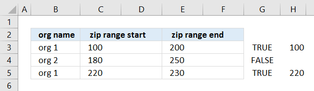
The IF function allows you to filter values, in this case a condition applied to cell range B3:B5 and return corresponding values in cell range C3:C5
IF($B15=$B$3:$B$5, $C$3:$C$5, "")
becomes
IF("org 1 "={"org 1 ";"org 2 ";"org 1 "},{100;180;220},"")
becomes
IF({"TRUE";"FALSE";"TRUE"},{100;180;220},"")
and returns the following array: {100; ""; 220}
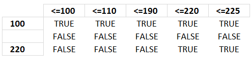
Step 2 - Compare with list
IF($B15=$B$3:$B$5, $C$3:$C$5, "")<=TRANSPOSE($B$8:$B$12)
becomes
{100; ""; 220}<=TRANSPOSE($B$8:$B$12)
becomes
{100; ""; 220}<={100,110,190,220,225}
and returns {TRUE, TRUE, TRUE, TRUE, TRUE; FALSE, FALSE, FALSE, FALSE, FALSE; FALSE, FALSE, FALSE, TRUE, TRUE}
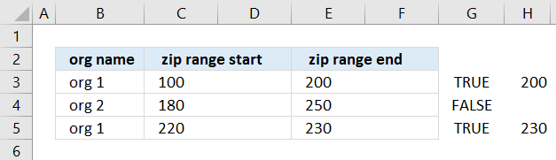
Step 3 - Filter end range values
IF($B15=$B$3:$B$5, $E$3:$E$5, "")
becomes
IF("org 1 "={"org 1 ";"org 2 ";"org 1 "},{200;"";230},"")
becomes
IF({"TRUE";"FALSE";"TRUE"},{200;"";230},"")
and returns the following array: {200;"";230}
Step 4 - Compare with list
IF($B15=$B$3:$B$5, $E$3:$E$5, "")>=TRANSPOSE($B$8:$B$12)
becomes
{200;"";230}>=TRANSPOSE($B$8:$B$12)
becomes
{200;"";230}>={100,110,190,220,225}
and returns {FALSE, FALSE, FALSE, TRUE, TRUE;FALSE, FALSE, FALSE, FALSE, FALSE;FALSE, FALSE, FALSE, FALSE, FALSE}
Step 5 - Filter values
Multiplying both logical expressions gives this formula:
IF((IF($B15=$B$3:$B$5, $C$3:$C$5, "")<=TRANSPOSE($B$8:$B$12))*(IF($B15=$B$3:$B$5, $E$3:$E$5, "")>=TRANSPOSE($B$8:$B$12)), TRANSPOSE($B$8:$B$12), "")
becomes
IF({TRUE, TRUE, TRUE, TRUE, TRUE; FALSE, FALSE, FALSE, FALSE, FALSE; FALSE, FALSE, FALSE, TRUE, TRUE}*{FALSE, FALSE, FALSE, TRUE, TRUE;FALSE, FALSE, FALSE, FALSE, FALSE;FALSE, FALSE, FALSE, FALSE, FALSE}, TRANSPOSE($B$8:$B$12), "")
becomes
IF({1,1,1,0,0;0,0,0,0,0;0,0,0,1,1}, TRANSPOSE($B$8:$B$12), "")
becomes
IF({1,1,1,0,0;0,0,0,0,0;0,0,0,1,1}, {100,110,190,220,225}, "")
and returns this array:
{100,110,190,"","";"","","","","";"","","",220,225}
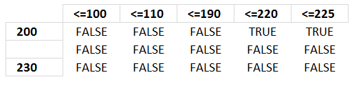
The following picture shows an index table that has values horizontally and what range they are in.
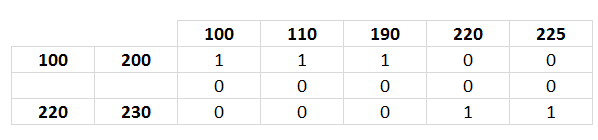
Example, values in range 100-200 are 100, 110 and 190 because the array has number 1 (TRUE) in those locations.
Step 6 - Find the k-th smallest value
SMALL(IF((IF($B15=$B$3:$B$5, $C$3:$C$5, "")<=TRANSPOSE($B$8:$B$12))*(IF($B15=$B$3:$B$5, $E$3:$E$5, "")>=TRANSPOSE($B$8:$B$12)), TRANSPOSE($B$8:$B$12), ""), COLUMNS($A$1:A1))
becomes
SMALL({100,110,190,"","";"","","","","";"","","",220,225}, COLUMNS($A$1:A1))
becomes
SMALL({100,110,190,"","";"","","","","";"","","",220,225}, 1)
and returns 100 in cell C15.
9.4. Excel *.xlsx file
More than 1300 Excel formulasExcel categories
30 Responses to “How to return a value if lookup value is in a range”
Leave a Reply
How to comment
How to add a formula to your comment
<code>Insert your formula here.</code>
Convert less than and larger than signs
Use html character entities instead of less than and larger than signs.
< becomes < and > becomes >
How to add VBA code to your comment
[vb 1="vbnet" language=","]
Put your VBA code here.
[/vb]
How to add a picture to your comment:
Upload picture to postimage.org or imgur
Paste image link to your comment.
Great post, Oscar. There are simpler formulas to do this, though.
=VLOOKUP($D$8,$B$4:$D$6,3,TRUE)
or
=INDEX($D$4:$D$6,MATCH(D8,$B$4:$B$6,1))
will also return B.
Thumbs up!!
I guess the columns must be sorted ascending in order for the formulas to work properly.
Thanks for your contribution!
[...] Return value if in range in excel, Oscar shows us a formula for returning values in a column based on a number range. Let's review [...]
happened upon this while calulating rating scores for timed surgical evaluation... needed formula to output score based upon time ranges... "formula in cell D10" worked perfectly! Thanks SO much!!!!
~charmain~,
I am happy you found it useful!
I am looking at a way to create a Bring Forward system witht the dates of the calendar.
It would be the first wednesday of the year like 2012-01-04 to 2012-01-18 would return the value of 1, and 2012-01-19 to 2012-02-01 would return the value of 2, etc...
Hi Oscar,
I came across this amazing formula when i was trying get a value return in a range:
INDEX(D4:D6, SUMPRODUCT(--($D$8=B4:B6), ROW(A1:A3))) + ENTER
But could not understand the usage of "--" in the sumproduct and also the logic behind using sumproduct itself.
Could you please help me to understand
Logical function (i.e. =46) you will always get numeric value 0. You can not convert FALSE to anything else other than numeric value 0.
It is not common to use more than two dashes since it can mess up your TRUE result (i.e. =---------------(TRUE) will return numeric value -1)
Logical function (i.e. =4 is less than 6) will return TRUE or FALSE value.
If you add one dash (-) in front of this logical function the result is the opposite (negative) value in numeric form; in this case result is -1
So if you add two dashes (--) in front of this logical function - the result is the opposite of the opposite (negative of the negative) in numeric form; in this case result is 1
The whole point is to easily convert result TRUE to numeric value 1, or convert result FALSE to numeric value 0.
p.s. of course, if you add as many dashes in front of logical function which results FALSE (i.e. =4 is more than 6) you will always get numeric value 0. You can not convert FALSE to anything else other than numeric value 0.
It is not common to use more than two dashes since it can mess up your TRUE result (i.e. =---------------(TRUE) will return numeric value -1)
Brilliant solution
I'm using the first formulation, but it assumes that the value fits between exactly 1 of the ranges. If it fits none, it returns the same value (which is not a big problem). If it fits on several ranges, it returns an error.
How do get it to provide at least one of the possible ranges instead of an error when there are several possible ranges?
Thanks!
Karl,
Array formula:
Attached file:
Return-value-if-in-range-karl.xls
Good day sir.
=INDEX(Calculate!D2:D6,SUMPRODUCT(--(Calculate!$D$9=B2:B6),ROW(Calculate!A1:A5)))
As you can see, I'm trying to put the formula to another sheet. Unfortunately I'm getting #value error.
Please advice, thank you.
Maybe oversimplifying it but wouldn't this solve your vlookup problem?
https://www.excelvlookuphelp.com/how-do-i-use-a-vlookup-where-the-range_lookup-is-true-rather-than-looking-for-an-exact-value-looking-for-a-range/
I have been searching for such formula...
May i know hot to do if value columns are more than one like Value-I, Value-II,Value-III and inputs are number and value type
Data is Range-I|Range-II|Value-I|Value-II|Value-III
Inputs are Number|Value-I
A formula which matches range of numberical input and match value type and copies the intersecting value...
To be simple two way lookup.
Hi
What if I want to use the same formula, but to change the range of the two columns B and C to be date range (07/01/2006 , 06/30/2007), and to change the value of column D to be a percentage (%450)
How can I use this formula please?
Alternatively this formula can also be applied:-
=LOOKUP(2,1/(($A$1:$A$3=F2)),$C$1:$C$3)
The first '2' represents the number of column to be searched for.
the expression '1/' represents the column number in the array.
'*' represents AND command.
The command will check the condition of whether F2 is greater than or equal to the values mentioned in the column 1. and then checks the condition that F2 is less than the value mentioned in the column 2 in the same row. Then displays the value corresponding to the same row in the column C.
Thank you all
It worked
I mean this: "=VLOOKUP($D$8,$B$4:$D$6,3,TRUE)"
I think it was the best solution
Hi All
I need some help to add rows to a spreadsheet based on the input of the user.
I ask the user to input the number of rows they need to add by inputting the value into a cell k6. Ideally I'd like them to press a nacro button which would the add the specified number of rows below row 8, keeping the same formulas in E8, G8, H8 and I8.
Can anyone assist?
ian
Hi Ian,
I made a workbook for you:
https://www.get-digital-help.com/wp-content/uploads/2010/01/Ian-inset-rows.xlsm
I continue to get #NAME? result using the first formula
My formula is:
=INDEX(F77:F80, SUMPRODUCT(--($D$83=D77:D80), ROW(A1:A4))) + ENTER
$D$83 is the Weight of a product, in numerical format.
Where F77:F80 is a list of prices (based on weight breaks)
D77:D80 is the min weight in a weight range
E77:E80 is the max weight in a weight range
As example of what would be in D77:F80
200,000 | 299,999 | 14.05
300,000 | 349,999 | 13.10
400,000 | 449,999 | 15.60
350,000 | 399,999 | 13.50
IF D83 is 330,327.
The result should be 13.10
Any advice?
I'm trying to create a formula in 4 different cells ”G3 – G6”, to search a column “B3 – B32” (ie: 4/1/17 – 4/30/17) filled w/dates and add a value from column “C3 – C32” if the date falls between the specified date range (ie: cell G3 reads column "B" for dates between 4/1-4/7, cell G4 reads column "B" for dates between 4/8-4/14, cell G5 reads column "B" for dates between 4/15-4/21 & cell G6 reads column "B" for dates between 4/22-4/30).
Hi. Can you please help me. I already have the IF formula where i want to generate a specific value from a column if between two dates.
Example:
Column A1 Start Date, Column B1 End Date, Column C1 Headcount
Data in 2nd row: Start date Jan. 1, 2014 up to Jan.31, 2015, headcount of 7.
FOrmula in Column D2:
=IF(AND(D1>=A2, D1 <= B2, C2, "")
The formula is working fine but the problem is when there is blank or no date in End date column, no value is returned. I would like to return the value in C2 whether there is end date or not. I would like to make use of one formula only that will work whether the End date has data or not.
Your help is very much appreciated. Thanks
JD,
Try this formula:
=IF((D1>=A2)*(D1<=B2)+(D1=""), C2, "")
i have query regarding returning multiple value against multiple checking and where i found value yes i have to return header row value by concatenate . example value
Mismatch - Recipient GSTIN Mismatch - GSTIN of the Supplier Mismatch - Invoice/Debit Note/ Credit Note (No) Mismatch - Invoice/Debit Note/ Credit Note (Date) Mismatch - Original Invoice No Mismatch - Original Invoice Date Mismatch - POS Mismatch - Supply attract reverse charge Mismatch - Total GST Rate Mismatch - Taxable Value Mismatch - IGST (Amt) Mismatch - CGST (Amt) Mismatch - SGST/UTGST (Amt) Mismatch - Cess(Amount)
No No No No No Yes Yes No No No Yes Yes Yes No
No No No yes No Yes Yes No No No Yes Yes Yes No
Hello Oscar,
I hope you are healthy and well in these troubled times.
re: https://www.get-digital-help.com/return-multiple-values-if-in-range-in-excel/
This doesn't work in Excel 2013 (or whichever one uses "|" instead of "," to separate arguments). Can you give me an update on what an updated version of your formula would be? Thank you very much!
great , this article is and excel file was the exact help i was looking for thanks for this brilliant article
Hi Oscar
I have two columns of numbers one is lower and one is higher. I have a third column with single numbers. I want to see if the third number is within the range of the two columns. If it is I just want it to say true. But I want check all of the ranges not just the ones across from them.
Any help would be very appreciated.
I have a range of data in 3 columns (B2:G6) and I want to find a value within B2:D6 and return a value that is exactly 4 cells to the right. How can I accomplish that?
Thanks in advance!