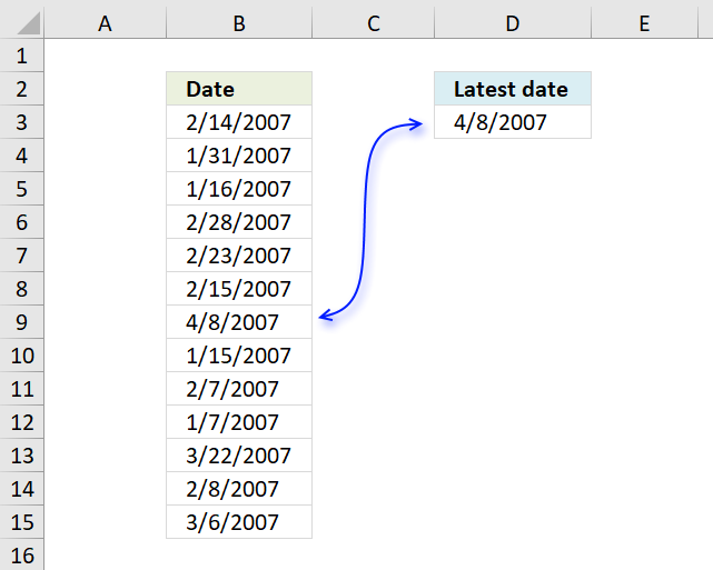
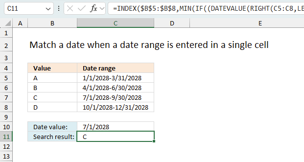
Find the most recent date that meets a particular condition

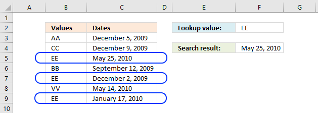
This article demonstrates how to return the latest date based on a condition using formulas or a Pivot Table. The condition is specified in cell F2 and the result is in cell F4.
For example, the condition is met in cells B5, B7, and B9. The corresponding dates in column C on the same row are 8/1/2022, 9/6/2022, and 7/29/2022.
The formula returns 9/6/2022 in cell F4 which is the last date of these dates.
Table of contents
- Lookup a value and find the most recent date
- Lookup a value and find the most recent date (Pivot Table)
- Lookup all values and find the most recent dates
- Lookup and find the most recent date using multiple conditions
- Lookup and find the most recent date on multiple sheets
- Lookup and find the most recent date, return another value on the same row
- Find the most recent date in a list
- List values with past date
- Lookup the nearest date
- Lookup min max values within a date range
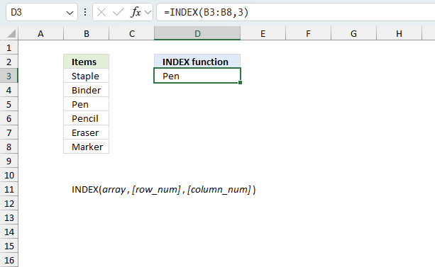
1. Lookup a value and find the most recent date
The picture above shows you values in column B (B3:B9) and dates in column C (C3:C9). The formula in cell F4 lets you search for value and return the latest date in an adjacent or corresponding column for that value.
1.0.1 Regular formula
Update, 2017-08-15! Added a regular formula.
The following formula is a regular formula, it is somewhat more complicated to understand, however, regular formulas are not prone to errors like array formulas. For example, inexperienced Excel users may easily break array formulas.
Formula in cell F4:
1.0.2 Array formula
The following formula is an array formula, section 1.2 explains how to enter an array formula.
Array formula in F4:
Section 1.3 explains how the formula above works in great detail.
How to create an array formula
1.0.3 Excel 2019 - regular formula
Formula in cell F4 (Excel 2019):
The MAXIFS function was introduced in Excel 2019, it is entered as a regular formula. You need Excel 2019 or a later Excel version to use this function.
1.0.4 Excel 365 formula
Update, 2021-09-09! Added an Excel 365 formula.
Formula in cell F4 (Excel 365):
The FILTER function is a new great function introduced in Excel 365.
1.1 Watch a video where I explain the formulas
Recommended article:
Recommended articles
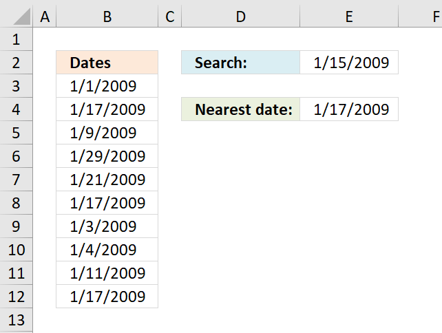
Table of Contents Lookup the nearest date Lookup min max values within a date range 1. Lookup the nearest date […]
1.2 How to create an array formula
The formula in 1.0.2 is an array formula and here are the steps to enter an array formula:
- Double press with left mouse button on cell C5.
- Copy / Paste above array formula.
- Press and hold Ctrl + Shift simultaneously.
- Press Enter.
- Release all keys.
The formula changes and now begins and ends with a curly bracket, don't enter these characters yourself. They appear automatically.
Recommended article:
Recommended articles

Array formulas allows you to do advanced calculations not possible with regular formulas.
1.3 Explaining array formula in cell C5
You can follow along if you select cell C5 and go to tab "Formulas" on the ribbon and then press with left mouse button on "Evaluate Formula" button. Press with left mouse button on "Evaluate" button, shown on the dialog box, to move to next step.
Step 1 - Find values equal to lookup value
The equal sign is a logical operator that lets you compare value to value, in this case, a comparison value to values is performed. The output is an array of boolean values.
C3=A8:A14
returns {FALSE; FALSE; ... ; TRUE}
Boolean values are either True or False, their numerical equivalents are True - 1 , False - 0 (zero).
Step 2 - Convert boolean values to corresponding dates
The IF function returns one value if the logical test is TRUE and another value if the logical test is FALSE.
IF(logical_test, [value_if_true], [value_if_false])
IF(C3=A8:A14, B8:B14)
returns {FALSE; FALSE; 40323; FALSE; 40149; FALSE; 40195}
Step 3 - Return the largest value
The MAX function allows you to calculate the largest number in a cell range. It ignores text, boolean and empty values, however, not error values.
MAX(number1, [number2], ...)
MAX(IF(C3=A8:A14, B8:B14))
returns 40323 formatted as 2010-05-25.
1.4 Excel file
2. Lookup a value and find the most recent date (Pivot Table)
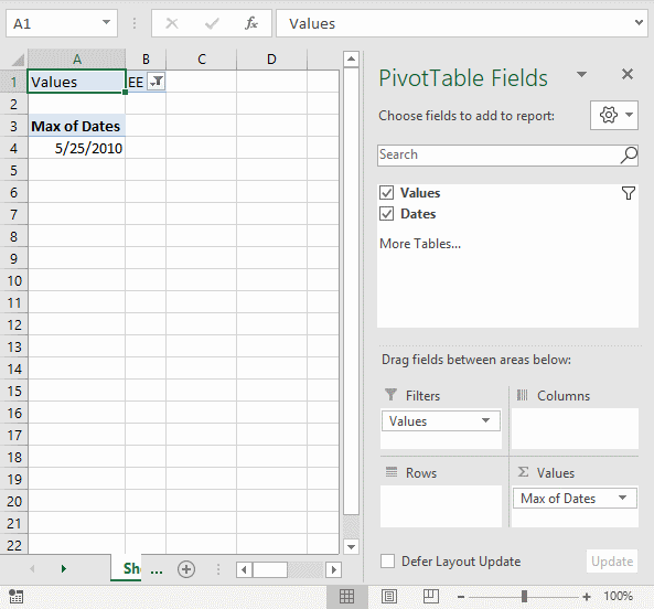
The formulas demonstrated in this article may be too slow or taking too much memory if you work with huge amounts of data. The Pivot Table is an excellent option in such cases, it is remarkably fast even with lots of data.
2.1 How to set up Pivot Table
- Select the cell range containing the data.
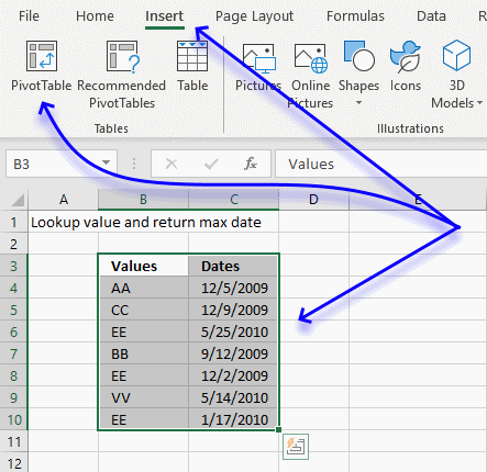
- Go to tab "Insert" on the ribbon.
- Press with mouse on "Pivot Table" button.
- A dialog box appears.
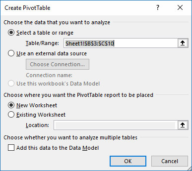
I usually place the Pivot Table on a new worksheet so it doesn't hide parts of the data set while filtering etc. - Press with left mouse button on OK button.
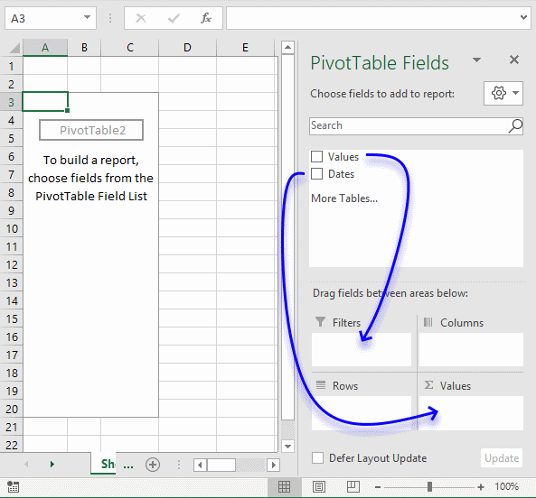
- Press with mouse on Values and drag to Filters field, see blue arrow above.
- Press with mouse on Dates and drag to Values field.
- Press with mouse on "Count of Dates".
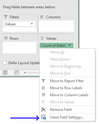
- Press with mouse on "Value Field Settings...".
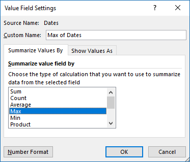
- Press with mouse on "Max" to select it.
- Press with mouse on "Number Format" button.
- Press with mouse on category "Date" and select a type.
- Press with left mouse button on OK button.
- Press with left mouse button on OK button.
Press with mouse on cell B1 to filter the latest date based on the selected value, the image above shows value EE selected and the latest date based on that value is 5/25/2010.
3. Lookup all values and find the most recent date
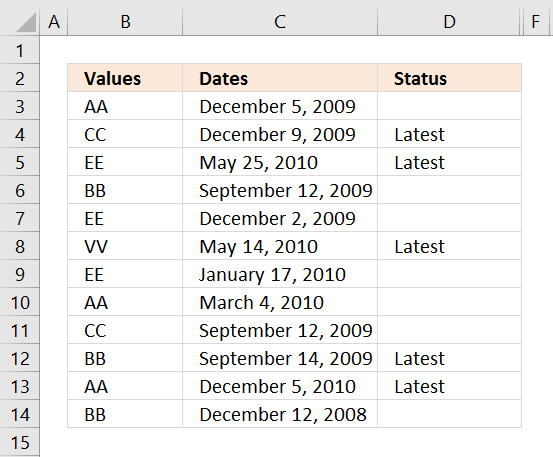
The following formula looks in column C for the most recent date based on the value in column B on the same row.
For example, cell B3 contains "AA". Cells B10 and B13 also contain "AA". The corresponding cells on the same row are C3, C10, and C13. They contain these dates "December 9, 2009", "March 4, 2010", and "December 5, 2010".
Cell D3 is not populated with the text "Latest", cell C3 is not the latest date. Cell C13 contains the last date based on the value "AA" in column B on the same row.
The following formula is a regular formula if you prefer that.
Formula in cell D3:
The next formula is an array formula, section 1.2 explains how to enter an array formula.
Array formula in cell D3:
The last formula contains an Excel 2016 function, MAXIFS function.
Formula in cell D3:
3.1 Watch a video explaining the formula above
3.2 How to copy array formula
- Copy cell C2
- Select cell range C3:C8
- Paste
3.3 Explaining formula
This section explains the array formula.
Step 1 - Identify cells that meet condition
The equal sign is a logical operator that compares value to value, it returns boolean values True or False.
B3=$B$3:$B$14
returns
{TRUE; FALSE; FALSE; ... ; FALSE}.
Step 2 - Replace boolean value with corresponding dates
The IF function returns one value if the logical test is TRUE and another value if the logical test is FALSE.
IF(logical_test, [value_if_true], [value_if_false])
IF(B3=$B$3:$B$14, $C$3:$C$14)
returns
{44554; FALSE; FALSE; ... ; FALSE}
Step 3 - Extract latest date
The MAX function allows you to calculate the largest number in a cell range. It ignores text, boolean and empty values, however, not error values.
MAX(number1, [number2], ...)
MAX(IF(B3=$B$3:$B$14, $C$3:$C$14))
returns 44559.
Step 4 - Compare with corresponding date on the same row
MAX(IF(B3=$B$3:$B$14, $C$3:$C$14))=C3
returns False.
Step 5 - Return "Latest" if True
IF(MAX(IF(B3=$B$3:$B$14, $C$3:$C$14))=C3, "Latest", "")
returns "" nothing in cell D3.
3.4 Excel file
4. Lookup and find the most recent date using multiple conditions

This example demonstrates a formula that uses two conditions to filter the latest date.
For example, the first condition is "Ram" and the second condition is "Pen". The formula calculates the latest date from column E if both conditions are true on the same row.
The first condition and the second condition are both found on rows 2 and 15, they are highlighted in the image above. The corresponding dates are 4/10/2017 and 11/1/2014, the latest date is 4/10/2017 which is returned in cell H3.
Formula in cell H3:
Array formula in cell H3:
How to create an array formula
4.1 Explaining array formula
Step 1 - First condition
The equal sign is a logical operator that compares value to value, it returns boolean values True or False.
D3:D30=I2
returns
{TRUE; FALSE; TRUE; ... ; TRUE}.
Step 2 - Second condition
E3:E30=I3
returns
{TRUE; TRUE; FALSE; ... ; FALSE}
Step 3 - Multiply arrays - AND logic
The asterisk lets you multiply arrays, this performs AND-logic meaning if both values are TRUE then return TRUE or their numerical equivalent 1. All other combinations return FALSE or 0 (zero).
The parenthesis lets you control the order of calculation, we want to compare values before we multiply the arrays.
(D3:D30=I2)*(E3:E30=I3)
returns
{1; 0; 0; ... ; 0}.
Step 4 - Replace boolean values with corresponding dates
The IF function returns one value if the logical test is TRUE and another value if the logical test is FALSE.
IF(logical_test, [value_if_true], [value_if_false])
IF((D3:D30=I2)*(E3:E30=I3),F3:F30,"")
returns
{42835; ""; ""; ... ; ""}.
Step 5 - Extract latest date
The MAX function allows you to calculate the largest number in a cell range. It ignores text, boolean and empty values, however, not error values.
MAX(number1, [number2], ...)
MAX(IF((D3:D30=I2)*(E3:E30=I3),F3:F30,""))
returns 42835 (4/10/2017) which is the largest number in the array.
4.2 Excel file
5. Lookup and find the most recent date on multiple sheets
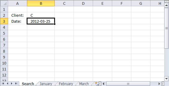
The picture above shows a workbook with 4 worksheets named "Search", January, February, and March. The formula in cell B3 looks for the latest date in all three worksheets using the condition in cell B2.
Unfortunately, it is not possible to use 3d references with IF functions. The formula contains three IF functions to make it possible to search all three worksheets.
Array formula in cell B3:
Update! Excel 365 dynamic array formula:
5.1 Explaining array formula
Step 1 - Logical test
The equal sign is a logical operator that lets you compare value to value. It is also possible to compare a value to multiple values in the same calculations, the result is an array of boolean values TRUE or FALSE.
B2=January!$B$2:$B$10
returns {FALSE; FALSE; ... ; TRUE}.
Step 2 - Filter dates from the worksheet named January
The IF function returns one value if the logical test is TRUE and another value if the logical test is FALSE.
Function syntax: IF(logical_test, [value_if_true], [value_if_false])
IF(B2=January!$B$2:$B$10, January!$A$2:$A$10, "")
returns {""; ""; 40929; ... ; 40914}.
Step 3 - Logical test
B2=February!$B$2:$B$10
returns {FALSE; FALSE; TRUE; ... ; TRUE}
Step 4 - Filter dates from the worksheet named February
The IF function returns one value if the logical test is TRUE and another value if the logical test is FALSE.
Function syntax: IF(logical_test, [value_if_true], [value_if_false])
IF(B2=February!$B$2:$B$10, February!$A$2:$A$10, "")
returns {""; ""; 40962; ""; ""; 40950; ""; ""; 40966}.
Step 5 - Logical test
B2=March!$B$2:$B$10
returns {FALSE; FALSE; TRUE; ... ; TRUE}
Step 6 - Filter dates from worksheet named March
The IF function returns one value if the logical test is TRUE and another value if the logical test is FALSE.
Function syntax: IF(logical_test, [value_if_true], [value_if_false])
IF(B2=March!$B$2:$B$10, March!$A$2:$A$10, "")
returns
{""; ""; 40993; ""; ""; 40981; ""; ""; 40970}.
Step 7 - Calculate largest number from three arrays
The MAX function calculate the largest number in a cell range.
Function syntax: MAX(number1, [number2], ...)
MAX(IF(B2=January!$B$2:$B$10, January!$A$2:$A$10, ""), IF(B2=February!$B$2:$B$10, February!$A$2:$A$10, ""), IF(B2=March!$B$2:$B$10, March!$A$2:$A$10, ""))
returns 40993. (3/25/2012)
5.2 Lookup and find the most recent date on multiple sheets - Excel 365
Excel 365 dynamic array formula in cell B3:
5.3 Explaining Excel 365 dynamic array formula
Step 1 - Create 3D reference
Here is how to create a 3D reference in cell B3:
- Select cell B3.
- Type the equal sign (=) to start creating the formula.
- Select cell range A2:A10 from the first worksheet (January).
- Press and hold CTRL key.
- Press with left mouse button on the sheet tab of the last worksheet (March) that you want to reference.
Note: To create a 3D reference, all the worksheets must be in the same workbook.
This is what the cell reference should look like in cell B3.
=January:March!A2:A10
Step 2 - Merge values from given cell ranges
The VSTACK function combines cell ranges or arrays. Joins data to the first blank cell at the bottom of a cell range or array (vertical stacking)
Function syntax: VSTACK(array1,[array2],...)
VSTACK(January:March!A2:A10)
returns
{40935; 40912; 40929; ... ; 40970}
Step 3 - Create a logical array containing TRUE or FALSE based on the condition specified in cell B2
This part of the formula merges the values in cell ranges B2:B10 in worksheets from January to March.
The equal sign compares the values to the specified condition in cell B2, the result is a boolean array containing TRUE or FALSE.
VSTACK(January:March!B2:B10)=B2
becomes
{"A"; "B"; "C"; ... "C"}="C"
and returns
{FALSE; FALSE; TRUE; ... ; TRUE}.
The semicolon ; is a row delimiting character in Excel arrays.
Step 3 - Filter dates based on the condition specified in cell B2
The FILTER function extracts values/rows based on a condition or criteria.
Function syntax: FILTER(array, include, [if_empty])
FILTER(VSTACK(January:March!A2:A10),VSTACK(January:March!B2:B10)=B2)
returns {40929; 40920; 40914; 40962; 40950; 40966; 40993; 40981; 40970}.
Step 4 - Get the latest date
The MAX function calculate the largest number in a cell range.
Function syntax: MAX(number1, [number2], ...)
MAX(FILTER(VSTACK(January:March!A2:A10),VSTACK(January:March!B2:B10)=B2))
returns 40993. 40993 represents the date 3/25/2012 in Excel.
5.4 Get Excel file
6. Lookup and find the most recent date, return the corresponding value on the same row
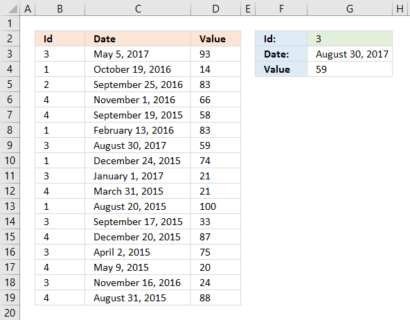
Enter a condition in cell G3, the formula extracts the latest date. Another formula in cell G3 gets the corresponding value on the same row from column D.
Array formula in cell G3:
If you prefer a regular formula in G3:
Update! New array formula in cell G4:
Excel 365 formula in cell G4:
Old Formula in cell G4:
6.1 Watch a video explaining the formulas above
6.2 Explaining formula in cell G4
Formulas in cell G3 are explained in section 1 above.
Step 1 - First condition
The equal sign is a logical operator that lets you compare value to value or in this case value to an array of values. The result is an array of boolean values TRUE and FALSE.
This logical expression compares the condition specified in cell G2 to the values in B3:B19.
B3:B19=G2
returns {TRUE; FALSE; FALSE; ... ; FALSE}.
Step 2 - Second condition
C3:C19=G3
returns {FALSE; FALSE; FALSE; ... ; FALSE}
Step 3 - Multiply arrays to perform AND logic
The asterisk character lets you multiply numbers in an Excel formula. The parentheses lets you control the order of operation.
(B3:B19=G2)*(C3:C19=G3)
returns {0; 0; 0; ... ; 0}
Step 4 - Find the relative position
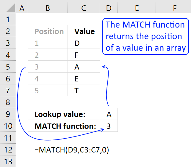
The MATCH function returns the relative position of an item in an array that matches a specified value in a specific order.
Function syntax: MATCH(lookup_value, lookup_array, [match_type])
MATCH(1,(B3:B19=G2)*(C3:C19=G3),0)
returns 7. Number 1 is in position 7 in the array.
Step 5 - Get value based on the relative position
The INDEX function returns a value or reference from a cell range or array, you specify which value based on a row and column number.
Function syntax: INDEX(array, [row_num], [column_num])
INDEX(D3:D19,MATCH(1,(B3:B19=G2)*(C3:C19=G3),0))
returns the value in cell D9 which is 59.
Find the most recent date in a list
The image above shows a formula in cell D3 that extracts the most recent date in cell range B3:B15.
The MAX function returns the largest number since Excel treats dates as numbers this will work fine. Number 1 is 1/1/1900 and 1/1/2000 is 36526. 1/2/2000 is 36527.
To extract the earliest date use the MIN function:
This returns 1/7/2007 from the list shown above.
To get the 3rd latest date use the following formula:
The LARGE function extracts the k-th largest number in a cell range. k is the second argument in the LARGE function.
To get the second earliest date use the SMALL function:
1/15/2007 is the second earliest date.
![]()
If you want to know where specific date is compared to the other dates in a list use the RANK function , in other words, if you were to sort the dates from largest to smallest where in the list would a specific date be located?
For example, 2/14/2007 would be the seventh date if the list shown above were sorted from largest to smallest.
Formula in cell B3:
The first argument in the rank function is the value you want to know the rank of. The second argument is the values you want it to be compared with.
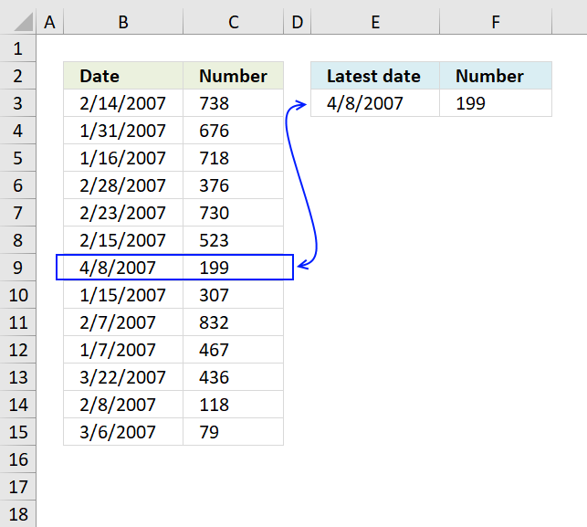
The image above demonstrates a formula in cell F3 that returns the corresponding value on the same row as the latest date is found.
The MATCH function returns the position of the value in cell E3 in cell range B3:B15. It returns 7 because 4/8/2007 is in the seventh position in cell range B3:B15.
INDEX(C3:C15, MATCH(E3,B3:B15,0))
becomes
INDEX(C3:C15, 7)
The INDEX function then returns the value in the seventh position in cell range C3:C15 which is 199.
8. List values with past date

Excel 365 dynamic array formula in cell E6:
Array formula (older Excel versions) in E6:
Formula (older Excel versions) in F6:
To enter an array formula, type the formula in a cell then press and hold CTRL + SHIFT simultaneously, now press Enter once. Release all keys.
The formula bar now shows the formula with a beginning and ending curly bracket telling you that you entered the formula successfully. Don't enter the curly brackets yourself.
Explaining formula in cell E6
Step 1 - Find rows in cell range with date past
Dates in Excel are numbers formatted as dates. 1/1/1900 is 1. 1/1/2000 is 36526. If you enter a date in a cell Excel automatically converts and formats the date, however, if you enter a date in a formula you need to use the DATE function to convert the date to an Excel date.
$C$3:$C$13<$F$3
returns {FALSE; FALSE; TRUE; ... ; TRUE}.
Step 2 - Convert TRUE to corresponding row number
The following IF function returns the row number if date number is less than number in cell F3. FALSE returns "" (nothing).
IF($C$3:$C$13<$F$3,ROW($C$3:$C$13)-MIN(ROW($C$3:$C$13))+1,"")
returns {"";"";3; 4;"";"";""; "";9;10; 11}
Step 3 - Extract k-th smallest row number
The SMALL function makes sure that a new value is returned in each row, the second argument $F$6:F6 is expanding when you copy the cell and paste to cells below. This adds 1 to the second argument for each cell below.
SMALL(IF($C$3:$C$13<$F$3, ROW($C$3:$C$13)-MIN(ROW($C$3:$C$13))+1, ""), ROWS($F$6:F6))
becomes
SMALL({"";"";3;4; "";"";"";"";9; 10;11}, 1) and returns 3.
Step 4 - Return value
The INDEX function returns a value based on a row and column number. Our cell range is only one column so we need only the row number to get the correct value.
INDEX($B$3:$B$13,SMALL(IF($C$3:$C$13<$F$3,ROW($C$3:$C$13)-MIN(ROW($C$3:$C$13))+1,""),ROWS($F$6:F6)))
returns "Williams" in cell E6.
Explaining formula in cell F6
Step 1 - Find adjacent value in cell range
COUNTIF(E6,$B$3:$B$13)
returns
{0;0;1;... ;1}
Step 2 - Find rows with date past today
($C$3:$C$13<$F$3)
returns
{FALSE; FALSE; TRUE; ... ; TRUE}
Step 3 - Multiply arrays
COUNTIF(E6,$B$3:$B$13)*($C$3:$C$13<$F$3)
returns {0;0;1;... ;1}.
Step 4 - Replace TRUE with corresponding row number
IF(COUNTIF(E6,$B$3:$B$13)*($C$3:$C$13<$F$3), MATCH(ROW($B$3:$B$13), ROW($B$3:$B$13)),"")
returns {"";"";3;... ;11}.
Step 5 - Extract correct row number
The second argument in the SMALL function contains the COUNTIF function, it is designed to count how many times the adjacent value has been displayed before. The first cell reference in the COUNTIF function expands as the cell is copied to cells below. This lets the formula keep track of previous values, we want it to return the correct date value even if there are duplicates in column B.
SMALL(IF(COUNTIF(E6, $B$3:$B$13)*($C$3:$C$13<$F$3), MATCH(ROW($B$3:$B$13), ROW($B$3:$B$13)), ""), COUNTIF($E$6:E6,E6))
returns 3.
Step 6 - Return date value
INDEX($C$3:$C$13, SMALL(IF(COUNTIF(E6, $B$3:$B$13)*($C$3:$C$13<$F$3), MATCH(ROW($B$3:$B$13), ROW($B$3:$B$13)), ""), COUNTIF($E$6:E6, E6)))
returns "10-Aug" in cell F6.
Get Excel *.xlsx file
List names whos date has pastv2.xlsx
9. Lookup the nearest date
The image above demonstrates an array formula in cell E4 that searches for the closest date in column A to the date in cell E2.
Array formula in E4:
Recommended articles:
Recommended articles
Table of Contents Find date range based on a date Sort dates within a date range Create date ranges that […]
Recommended articles
This article explains how to search for a specific date and identify a date range in which it falls between […]
How to enter an array formula
- Select cell E4
- Type or copy/paste above array formula to formula bar
- Press and hold Ctrl + Shift
- Press Enter
Learn more about array formulas:
Recommended articles
Array formulas allows you to do advanced calculations not possible with regular formulas.
Explaining array formula in cell E4
You can easily follow along, select cell E3. Go to tab "Formulas" and press with left mouse button on "Evaluate formula".
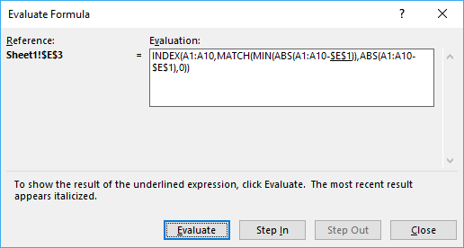
Press with left mouse button on "Evaluate" button to move to next step.
Step 1 - Subtract dates with search date
B3:B12-$E$2
returns {-14;2;-6;14;6;2;-12;-11;-4;2}
Step 2 - Convert numerical values to absolute values
The ABS function converts a negative number to a positive.
ABS(B3:B12-$E$2) returns {14;2;6;14;6;2;12;11;4;2}
Step 3 - Find smallest numerical value in array
The MIN function returns the smallest number in a cell range or array.
MIN(ABS(B3:B12-$E$2)) returns 2.
Step 4 - Find position in array
The MATCH function returns the relative position of a given value in an array or cell range.
MATCH(MIN(ABS(B3:B12-$E$2)), ABS(B3:B12-$E$2), 0)
returns 2. Numerical value 2 has position 2 in the array.
Learn more about the MATCH function:
Recommended articles
Identify the position of a value in an array.
Step 5 - Return value
INDEX(B3:B12, MATCH(MIN(ABS(B3:B12-$E$2)), ABS(B3:B12-$E$2), 0))
returns 39830 or 1-17-2009 in cell E4.
Learn more about the INDEX function:
Recommended articles
Gets a value in a specific cell range based on a row and column number.
Get excel example file
find-nearest-date.xls
(Excel 97-2003 Workbook *.xls)
Recommended articles:
Recommended articles
This article explains how to find the smallest and largest value using two conditions. In this case they are date […]
Recommended articles
This article demonstrates how to return the latest date based on a condition using formulas or a Pivot Table. The […]
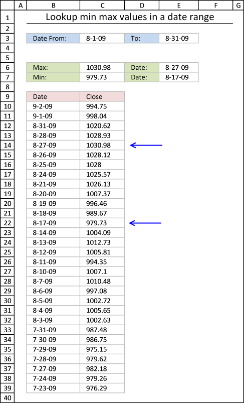
10. Lookup min max values within a date range
This article explains how to find the smallest and largest value using two conditions. In this case they are date conditions but they can be whatever you like, displayed in cell C3 and E3.
The maximum value in that date range is calculated in cell C6, The minimum value in cell C7. There is also a formula that finds these values and return their corresponding date, in cell E6 and E7.
Formula in cell C6:
The MAXIFS function returns the largest number from max_range ($C$10:$C$39) based on a condition or criteria.
MAXIFS(max_range, criteria_range1, criteria1, [criteria_range2, criteria2], ...)
The first condition $B$10:$B$39, "<="&$E$3 identifies rows whose date is smaller than or equal to date in cell E3.
The second condition $B$10:$B$39, ">="&$C$3 identifies rows whose date is larger than or equal to date in cell C3.
Formula in cell C7:
The MINIFS function works exactly the same as the MAXIFS function, however, the smallest number is instead returned.
Formula in cell E6:
This formula is a simple lookup formula, it returns only a single value from column B if the value in column C matches the contents of cell C6.
INDEX($B$10:$B$39,MATCH(C6,$C$10:$C$39,0))
The MATCH function returns the relative position of a value in a cell range or array.
INDEX($B$10:$B$39,MATCH(1030.98,$C$10:$C$39,0))
becomes
INDEX($B$10:$B$39,5)
The INDEX function returns a value based on a row (and column number if needed).
and returns 8-27-09 in cell E6.
Formula in cell E7:
Get excel *.xlsx file
Lookup min max values in a date range.xlsx
Dates category
Question: I am trying to create an excel spreadsheet that has a date range. Example: Cell A1 1/4/2009-1/10/2009 Cell B1 […]
This article explains how to search for a specific date and identify a date range in which it falls between […]
This article demonstrates a formula that points out row numbers of records that overlap the current record based on a […]
Dates basic formulas category
Question: I am trying to create an excel spreadsheet that has a date range. Example: Cell A1 1/4/2009-1/10/2009 Cell B1 […]
This article explains how to search for a specific date and identify a date range in which it falls between […]
Excel categories
161 Responses to “Find the most recent date that meets a particular condition”
Leave a Reply
How to comment
How to add a formula to your comment
<code>Insert your formula here.</code>
Convert less than and larger than signs
Use html character entities instead of less than and larger than signs.
< becomes < and > becomes >
How to add VBA code to your comment
[vb 1="vbnet" language=","]
Put your VBA code here.
[/vb]
How to add a picture to your comment:
Upload picture to postimage.org or imgur
Paste image link to your comment.
This is a great example. I was attempting to figure out how to get the greatest date based on a log on ID. This example fit the bill perfectly. Many thanks!!
Thanks for your comment!
Excellent example and explanation. This helped me tremendously and saved me a LOT of time. Thank you so much!
Brent,
Thanks for commenting!
Totally agree, I haven't used arrays before and this was a great intro. Thanks!
JS,
thanks! I wrote an explanation.
Great info. My scenario is slightly different. I'd like the result to come up in each row in column C. If the date is MAX for that rows value(column A) then say "Newest" else blank.
ie. C8 would result "Newest" AA is the only instance on the list. C10 would result "Newest" as it has the MAX date for all the EE's. Consequently C12 and C14 would result Blanks as it is not the MAX date.
Any help would be appreciated.
Albert S,
Great question, I added new content to this post: Lookup all values and find max date
Hello,
Just stumbled across your post trying to find a solution and this was just perfect !
Thank you very much.
- Jyri
Jyri,
Thanks for commenting!
Thanks, this is just what I was after!
You are welcome!
Thank you! This is a lovely neat little formula.
Thank you for commenting!
Hi,
I am in desperate need of some help. I have column A with multiple dates against which I have REGISTRATIONS of FLEET CARS. I want to find and match the most recent date or the last date that a REG took a passengers fair. Any help would be much appreciated.
DATE CAB REG
1/26/2012 LT61ZND
1/26/2012 LT61ZND
2/25/2012 BO51CAB
2/25/2012 LM56FCO
2/25/2012 LM56FCO
2/25/2012 LP10FXU
2/25/2012 LP10FXU
2/25/2012 LL07FYV
2/26/2012 LS60YLG
2/26/2012 LM06WKD
2/26/2012 LG02UPP
2/26/2012 LT61ZND
2/26/2012 W198WGH
2/26/2012 LS51BKG
2/26/2012 LF53EVC
2/26/2012 LS51BKG
HI,
I forgot to mention that the Registrations of fleet cars are in column B.
many thanks,
Natway :-)
Natway,
I this what you are looking for?
This has been very helpful, however I need to be able to look through several sheets for the most recent date. Is that possible? I have my workbook set up with each month on a separate sheet. I'm trying to find the last appointment date for each of my clients.
erica,
Is that possible?
I am not sure, you would have to change the formula every time you add a sheet, unless you are allowed to use vba?
I wouldn't be adding any more sheets. I'm not sure how to wright the formula to look through all the sheets. I'm a bit of a novice at excel. I'm not sure what vba is either.
erica,
https://www.get-digital-help.com/lookup-a-value-and-find-max-date-in-excel/#multiplesheets
Eureka! Thank you, thank you. I knew there had to be a way.
Hello, this is great but i need to get the most recent value in a list of dates. For example, in the ist below I need to be able to get the most recent value (either 1,2,or 3) posted for the quarter.
Quarter Date Value
4 12/5/2012 1
4 12/5/2012 3
1 1/3/2012 2
1 2/15/2012 3
2 4/13/2012 1
2 3/12/2012 3
3 7/25/2012 1
3 9/2/2012 2
Here is the formula I am currently using which is averaging the numbers, dont need to do that anymore. I only need to get the most recent value for a given quarter.
=SUM(IF(COUNTIF(Q127:Q130,1)=0,1,AVERAGEIF(Q127:Q530,1,S127:S530)))
Eugenious1,
https://www.get-digital-help.com/lookup-a-value-and-find-max-date-in-excel/#return
Hello oscar, i have tried your second example, but everytime i try it i only get a newest entered where the cells is equal to EE, all other values show a blank, unlike yours where each unique value of the A column shows that to be the newest entry. Why is that?
Subash,
Did you enter the formula as an array formula?
=IF(MAX(IF(A2=$A$2:$A$8, $B$2:$B$8))=B2, "Newest", "")
The formula returns "Newest" if it is the latest record.
Example,
EE has three entries and only the latest date returns "Newest". The other values are unique and returns "Newest".
Below is the formula I am using. Can you tell me what I did wrong?
Column O is the value I want to look up (103046)
Column C is the range I am looking O up in
Column E is the result I want (which should be the most recent date) (answer is 8/20/12)
The answer for this should give me 8/20/12 and I keep getting 12/13/12. I have formatted both date columns the same.
=MAX(IF(O3=C3:C50,E3:E50,""))
So I believe it is giving me the max date in column E not the maximum date in E that relates to the value I am looking up. Any help with a formula?
Column C Column E
103046 8/20/12
103046 6/10/11
103046 1/10/11
108003 12/13/12
108139 12/12/12
122007 5/06/11
122007 8/1/12
Angie,
Your array formula is fine, I don´t think you have entered the formula as an array formula.
See array formula instructions above in this post.
Hello Oscar,
Thanks again, i did realize that mistake i was making and got it corrected, it worked perfectly. :-)
Hi Oscar,
I am trying your formula
=MAX(IF(D38=B4:B32,J4:J32))
but I am getting #value error
Also I use
=MAX(IF(D39='Sheet1'!$B$4:$B$32,'Sheet1'!$J$4:$J$32))
Then also I am getting same error
Nevermind its working now !!
when I followed these steps
3.Press and hold Ctrl + Shift
4.Press Enter
Now can you tell me why these steps are necessary and why it does not work without it ?
Hi Oscar, i am regularly following your site, really helped.
Name Target Announced Date Beneficiary Proceeds
Kiran Microsoft 2/13/2013 500
Kiran Microsoft 2/14/2013 200
Kiran Google 2/12/2013 500
Sriram Microsoft 2/12/2013 500
Sitaram Microsoft 2/12/2013 500
Based on Name, Target, latest date i need beneficiary Proceeds in a column.
I am trying in this way: 1) identifying latest date =MAX(IF($L$2:$L$50=L2,$M$2:$M$50))--But not getting for two column critria
2) Indexing based in latest date: =INDEX($S$2:$S$13,MATCH(1,($L$2:$L$13=L2)*($M$2:$M$13=X2)*($K$2:$K$13=K2),0))
2nd one is perfect and first one i am unable to get value based on two columns criteria.
Is there any alternate way to display Value based on multiple criteria (atleast 2) with latest entry.
Kiran,
Array formula in cell A12:
=MAX((A2:A6=A9)*(B9=B2:B6)*C2:C6)
Array formula in cell B12:
=INDEX($D$2:$D$6,MATCH(1,($A$2:$A$6=A9)*(B9=$B$2:$B$6)*(A12=C2:C6),0))
Dear oscar,
I need newest receiving date of any article when i have more than 500 articles.
Please suggest for it.
For exp
A 12-03-21
B 12-04-13
A 15-03-25
I have used above formula which was
=if(max(if a=a1:a3 etc
But it showing the last date in from the date column.
Pls help
This is absolutely great function. Many thanks for this.
However, if the any of the datevalues are blank or not properly formatted. The function wont work.
Perhaps could be easily fixed.
This has saved days of my work. I really appreciate your several contributions specially with Array functions.
Best wishes
Aziz
Aziz,
The formula works with blank datevalues.
Thank you for commenting!
Hi Oscar
I opened the excel file you provided and copied the exact same formula =INDEX(A1:A10, MATCH(MIN(ABS(A1:A10-$E$1)), ABS(A1:A10-$E$1), 0)).....it simply doesn't work for me, what is wrong with my input??
I would be appreciated if you could help ..do I have to be mindful of some settings?
Andrew,
You need to enter the formula as an array formula. Sorry for not being clear.
1. Paste the formula to the formula bar
2. Press and hold CTRL + SHIFT
3. Press Enter simultaneously
4. Release all keys
The formula in the formula bar should now have curly brackets, like this:
{=INDEX(A1:A10, MATCH(MIN(ABS(A1:A10-$E$1)), ABS(A1:A10-$E$1), 0))}
What if I need to return a date equal to or greater than the search date instead of the "nearest date"? Then, what if the dates don't contain a date that is equal or greater than the search date, can I pull back a blank?
Jeremy,
Array formula:
=INDEX(A1:A10, MATCH(MIN(IF(A1:A10-$D$1>=0, A1:A10-$D$1, "")), A1:A10-$D$1, 0))
Thank you for commenting!
Life saver just changed range to $A$2:$A$999 same for other.
Thanks
Zuber,
I am happy you find it useful.
I am looking for the formula where i can find maximum from column h based on values found matching in column c and column d.
I tried formula given by oscar but it didnot work and give error.
Please suggest
PARDEEP,
Did you enter the formula as an array formula?
Hi Oscar, i am regularly following your site.
how i pick the 37 & 34 & 18 & 15 ID series data with name and latest date visit other duplicates should be deleted.
ID Name ADD1 ADD2 ADD3 interview date
3706 jagdambaenim sdfsdfsd sdfsdf 7/16/2010
3405 ravi kaun sdfsdfsd sdfsdf 7/19/2012
1804 chandan jay sdfsdfsd sdfsdf 7/15/2011
1504 vikash sdf sdfsdfsd sdfsdf 1/18/2010
3706 jagdambajay sdfsdfsd sdfsdf 7/15/2010
3405 ravi enim sdfsdfsd sdfsdf 7/25/2012
1804 chandan sdf sdfsdfsd sdfsdf 7/15/2011
1504 vikash jay sdfsdfsd sdfsdf 1/5/2013
3706 jagdamba nima sdfsdfsd sdfsdf 7/19/2010
3405 ravi dfsdf sdfsdfsd sdfsdf 7/19/2012
1804 chandan nima sdfsdfsd sdfsdf 7/29/2011
1504 vikash dfsdf sdfsdfsd sdfsdf 7/15/2013
3706 jagdamba nima sdfsdfsd sdfsdf 7/13/2010
3405 ravi dfsdf sdfsdfsd sdfsdf 7/19/2012
Deepak,
I can´t come up with a solution for searching multiple text strings.
This one let´s you search for a single text string:
Array formula in cell A20:
Get the Excel *.xlsx file
Search-for-a-text-string-and-find-latest-records.xlsx
Oscar hi ,
I have tried all but I got #value error...why?
Sorry works with ctrl+shift+enter
but what is array formula ? Why do we need that ?
For along time excel user that is the first time I see
Thanks & Regards
jeam,
but what is array formula ? Why do we need that ?
You can do more complicated calculations. Try to lookup a value and find max date using regular formulas in one cell only.
How about finding a oldest date if the value is greater than 500for example.(see below)
Column A Column B
22-2-12 200
21-2-12 501
30-3-12 502
20-2-12 503
in this example, there is 3 items which is greater than 500 ( 501, 502, 503) with different date. And the oldest date seems to be 20-2-12. how can i show the oldest date using formula?
Please help, thank you
Louie,
Array formula in cell E2:
=MIN(IF(B1:B4>E1,A1:A4,""))
Thank you for commenting!
Fun fact I am proud of, as this thread introduced me to the array formula concept just a couple of hours ago, and it took a while to understand what parts of the formula returned what values. I wanted to use this to find nearest future date from a horizontal array (3 columns, 1 row). I made it work in your vertical array example by the array formula: =INDEX(A1:A10,MATCH(0,A1:A10-$E$1,-1),1). Then I copied, transposed, and pasted the date array into A12:J12 and changed the formula to: =INDEX(A12:J12,1,MATCH(0,A12:J12-$E$1,-1)). YAY!
Kris,
I wanted to use this to find nearest future date from a horizontal array (3 columns, 1 row). I made it work in your vertical array example by the array formula: =INDEX(A1:A10,MATCH(0,A1:A10-$E$1,-1),1)
Yes, you don´t need the ABS function in your example. Great!
Hi Oscar
I have a similar problem but with a twist.I have two worksheets and I need to lookup a date in a nearest date range.y data looks soething like this.
Data Date Data Date Result date
A 1/1/2013 A 1/5/2013 1/1/2013
A 2/1/2013 B 4/6/2013 4/1/2013
A 3/1/2013
B 4/1/2013
B 5/1/2013
So as you can see the formulae forst needs to match the two data columns like(A-A)and only then pick the nearest date corresponding to dates pertainig to that data point.
Hope I am clear.Kindly request you to help
Murtuza Vasanwala,
I am sorry, I don´t understand. Can you describe in greater detail?
Hi Oscar sorry for such a late reply but let me explain myself in greater detail.Basically I have two columns of data containing the same entries so assume column A and column C are two such columns.and column B and column D have certain dates corresponding to these entries.I need a formulae which will first match the entries in column A wih entries in column C .then compare the date in column D with the dates in column B and then throw up the nearest date.So my data sheet looks something like this:
Col A Col B Col C Col D Col E(result)
A 1/2/2013 A 5/1/2013 4/3/2013
A 2/2/2013 B 5/2/2013 5/5/2013
A 4/3/2013
B 5/5/2013
B 9/10/2013
As you can see the formulae first compares the entries in col C (A) with the entries in col A (all the A's) then it matches the date in col D (5/1/2013) with the dates pertaining to value A in col B.The closest date then is 4/3/2013 which is the answer.
Hope I have made myself amply clear this time waiting for your response
Murtuza vasanwala,
Read this:
https://www.get-digital-help.com/excel-find-closest-value/#criterion
I need to write a formula where I type in a date and it looks through a column and sees which date is it greater than but closest to.
Robert,
=INDEX(A1:A10, MATCH(MIN(ABS(If(A1:A10>=E1,A1:A10-E1,""))), ABS(If(A1:A10>=E1,A1:A10-E1,"")), 0))
Thank you for your excellent explanation!
Just had a slight moment of doubt, all the formula returned were zeros, but it was due to format of the values, I had them as Text.
As soon as I modified them to date it worked perfectly!
I was trying to work out a formula similar to this in that I had 2 columns on each sheet one column had names and the other dates same style on the other sheet. I want to find dates that were closest to each other for a specific name, but didnt work out. How can I tweak this formula to pull that off? It seems a bit tricky cause I couldnt resolve what to do in place of the $E$1 cell? Any suggestions?
Hi Oscar, i am regularly following your site.
how i pick the earliest date in the below given dates in 'A' for value more than 0 in 'B':
Date [A] Value[B]
03-11-2014 702,000.00
23-09-2014 0.00
07-10-2014 283,000.00
02-09-2014 0.00
08-12-2014 346,752.00
28-10-2014 347,375.00
05-11-2014 288,960.00
18-11-2014 290,298.18
17-09-2014 0.00
22-09-2014 0.00
15-09-2014 0.00
25-11-2014 286,383.00
22-12-2014 252,000.00
I have a cell at the top of my spreadsheet that mirrors the expiry date closest to today.
I am wondering if there is a way to have it link to the cell it is mirroring, rather than scrolling down through thousands of rows to find the highlighted cell in question?
To my opinion there is a much simpler NON-Array formula that achieves the same:
Michael (Micky) Avidan
=LOOKUP(2,1/FREQUENCY(0,ABS(A1:A10-E1)),A1:A10)
“Microsoft® Answers" - Wiki author & Forums Moderator
“Microsoft®” MVP – Excel (2009-2015)
ISRAEL
Micky,
thanks for sharing!
This worked like a charm. Thanks
How would you go about doing the above while excluding any values that happen to be zero?
Thomas
=MIN(IF((Date_col<=$E$3)*(Date_col>=$C$3)*(Close_col<>0), Close_col, ""))
Hi, I have 15 rows of varying dates. And I have a separate date on the 16th row. How can I determine the closest start date and the closest end date range that the 16th row date falls in?
Any help is much appreciated. Thank you.
-Bishnu
Example:
1.01/28/16
2.10/24/16
3.01/18/17
4.01/29/18
5.06/05/18
6.08/06/18
7.09/05/18
8.01/14/19
9.07/17/19
10.01/21/20
11.09/04/20
12.09/05/22
13.01/24/23
14.01/17/24
15.01/21/25
(Above varying dates)
16.3/26/2019
(To determine where this above date falls in between closest to)
17. Start Date =09/05/18
18. End date = 07/17/19
(How do I figure out 17. and 18.) Thanks, hope this example helps to understand the problem a bit more.
@Mayetreyee,
I would suggest as following formulas:
1) To determine the Lowest Closest date:
=MAX((A1:A15=0,A1:A15))
*** Both s=are Array-Formulas !!!
------------------------------
Michael (Micky) Avidan
“Microsoft® Answers" - Wiki author & Forums Moderator
“Microsoft®” MVP – Excel (2009-2015)
ISRAEL
@Mayetreyee,
Something went wrong in my previous reply.
I would suggest as following formulas:
1) To determine the Lowest Closest date:
=MAX((A1:A15=0,A1:A15))
2) To determine the Highest Closest date:
=MIN(IF(A1:A15-A16>=0,A1:A15))
*** Both are Array-Formulas !!!
------------------------------
Michael (Micky) Avidan
“Microsoft® Answers" - Wiki author & Forums Moderator
“Microsoft®” MVP – Excel (2009-2015)
ISRAEL
Hi
I have a problem. I need a formula that returns me the Code associated to the most recent date that has occurred for a particular ID number (the sheet is very long and will have the same ID multiple times. If I could get a formula to return the code for the most recent occurrence that would be amazing!
ID Date Code
1234 12/12/2013 F
2345 15/09/2013 R
3456 21/08/2014 R
1234 01/01/2014 P
I would want the code to bring back the code P.
I am using this Array formula at the moment but it does return the correct code for all, sometimes it picks up other codes.
=INDEX($C:$C,MATCH(MAX(IF(A2=$A:$A,$B:$B)),$B:$B,0))
Unsure, please help.
I went about this a little differently, no arrays needed
Find how many numbers are bigger then the one you are looking for with CountIf()
Then I used =Large this will find the nth dates in a list we have the nth we are looking for in the countIF()
=LARGE(A:A,COUNTIF(A:A,">="&TODAY()))
for the highest closest date =LARGE(A:A,COUNTIF(A:A,">="&TODAY()+1))
for the lowest closest date =LARGE(A:A,COUNTIF(A:A,">="&TODAY()-1))
https://www.excelireland.com
Dear all,
your advices are really helpful, I need the opposite of the comment (Jan, 30,2014) so smaller but closet to.
Thanks
Hello Oscar,
thank you for sharing you knowledge and helping us with these excellent formulas.
I have a case i could really need your help with:
The following Table shows a history of names, stati and the date the satus was acquired. BUT: people can acquire the same status more than just once (or at least report it). Now I want to know, when each person (peter, sarah & luke) have acquired their individual highest status.
Name Date Status
peter 30.01.2015 5
sarah 30.01.2015 5
peter 28.01.2015 5
sarah 28.01.2015 4
peter 24.01.2015 5
peter 22.01.2015 5
sarah 22.01.2015 3
luke 22.01.2015 4
peter 20.01.2015 3
sarah 20.01.2015 3
sarah 18.01.2015 2
peter 18.01.2015 2
luke 18.01.2015 3
luke 16.01.2015 3
luke 14.01.2015 2
peter 14.01.2015 2
peter 12.01.2015 1
sarah 12.01.2015 2
peter 10.01.2015 1
sarah 10.01.2015 2
sarah 08.01.2015 1
answers have to be :
Names latest status in status since
Peter 5 22.01.2015
sarah 5 30.01.2015
luke 4 22.01.2015
I would really appreciate your help.
Greetings.
Denis,
I made a post for you:
https://www.get-digital-help.com/find-the-highest-status-and-when-it-was-acquired/
[…] Denis asks: […]
Dear Oscar
I want to search Max date on Monthly and yearly basis
I used MAX with array but failed to get the desired results
Date Result I want Result I am getting
1-Jan-14 12-Dec-15
2-Jan-14 2-Jan-14 12-Dec-15
15-May-15 15-May-15 12-Dec-15
12-Dec-15 12-Dec-15
12-Dec-15 12-Dec-15 12-Dec-15
Regards,
Thanks for sharing how to find the nearest date. But I'm stuck with another condition that is I have another lookup value (some user ids) and only if that matches then I have to search for the nearest newest dates for that row. Please note that there are duplicate user ids.
Regards,
Ehsan
Dear Oscar
I need to return the earliest date for each ID number and would really appreciate your help as if I use any of the above calculations I can't get it to work.
ID No Date
2816746 16/06/2015
2816746 25/06/2015
2816746 16/07/2015
2816746 22/07/2015
2816746 28/07/2015
5269339 11/08/2015
5269339 14/08/2015
5269339 30/09/2015
7088617 22/06/2015
7088617 21/07/2015
7451444 15/06/2015
7451444 30/07/2015
7608629 15/07/2015
7608629 10/08/2015
7608629 11/09/2015
7608629 06/10/2015
8183184 06/08/2015
8261932 14/10/2015
Kind regards
You are a lifesaver! I've been trying to figure this out for hours, until I came across your site.
What does the asterisk do in the formula? I know it's not multiplying anything, but I have never seen it this way.
=MIN(IF((Date_col=$C$3)*(Close_col0), Close_col, ""))
Mark McPherson,
Thank you!
The asterisk multiplies two arrays.
Example, (TRUE, TRUE, FALSE)*(TRUE, FALSE, FALSE) equals (1,0,0).
1 = TRUE
0 = FALSE
We are a bunch of volunteers and starting a new scheme in our community.
Your site provided us with helpful info to work on. You have performed
an impressive task and our whole group might be grateful to you.
This is what i've been trying to figure out for a while. eloquent statement, detailed explanation...you've really opened my eyes to the power of arrays!
do you have a paypal that i can leave a MODEST donation?
Excellent :)
=MAX(IF((C3=A8:A14;D3=C8:C14);B8:B14;0))
no work in code with muli cons.
=MAX(IF((C3=A8:A14;D3=C8:C14);B8:B14;0))
Lookup value and return max date
Lookup value: EE ok
Search result: #VALUE!
Values Dates
AA 05/12/2009 yes
CC 09/12/2009 no
EE 25/05/2010 no
BB 12/09/2009 no
EE 09/03/2016 yes
VV 14/05/2010 no
EE 17/01/2010 no
=MAX(IF(AND(C3=A8:A14;D3=C8:C14);B8:B14;0))
Hi Oscar, Thanks for your useful post. I have a question...
MY DATE: 2016/02/03
A B C= quantity
1 2016/02/01 BAG 10
2 2016/02/02 BAG 20
3 2016/02/02 Tie 30
4 2016/02/03 BAG 70
5 2016/02/03 BAG 65
6 2016/02/03 BAG 50
7 2016/02/04 BAG 60
I want to lookup LAST quantity from Bag goods at 2016/02/03, in the other hand cell C6=50
Thanks in advance your Reply
Alex,
Array formula in cell B10:
=INDEX($C$1:$C$7, MAX(IF(A10=$A$1:$A$7, MATCH(ROW($A$1:$A$7), ROW($A$1:$A$7)), "")))
This is incredible info. Thank you!
If there are repeated values in the close column, the expression returns the first occurrence of the value, regardless of the identified data range. how do we modify the formula to return the value in the date range identified?
Hi I try this formula. But it is not work for me. It shows True rather than {True,False,False,True} format.
thanks a lot! I am actually learning a lot in this website! Now my Excel skills are surely definitely improved ;) this website is so good!
For example: I say, 01.03.2016 - 31.05.2016 between the dates the book 5 usd. 01.06.2016-31.07.2016 between the dates the book 10 usd.How do you write a formula that he wrote any date range (05.04 2016 or 08.06.2016), and wrote the book price will come automatically.
Thanks for the great tips!!
Is it possible to nest this to exclude matches with a "Closed" status in another column?
I have the ranges "Helper1Date" in column A, "woRef" (result data) in column D, and "Status" in column I and I need to return the WORef # for items dated today or older that do not have the status "Closed" (value "Closed" pasted to C1).
I also have a couple other status labels pasted to D1 and E1 that I'd like to exclude, but if I can at least exclude C1 "Closed" that would help a lot!
Hi Oscar,
Please help me.
I need to get the most latest expiration date of my projects but i dont know how to do it.
https://postimg.org/image/gvxln5ww3/
Assuming the columns are a through e. Also assume that the first line of data is on row 5:
=max(if(d5=a5:a20,b5:b20))
Press ctrl shifty enter
Drag down as needed
*consider using data as tables...it makes updates seamless...because you'd be referencing a column not a range that had to be updated
Hi Oscar
I am trying to lookup the nearest activity date to a target date based on ID number. For ID 01 the closest date would be 05/07/2016. Therefor everytime the ID changes the range to lookup and compare will be different. Are you able to advise on solving this task.
ID Target Date ActvityDate
01 12/07/2016 05/07/2016
01 12/07/2016 15/08/2016
01 12/07/2016 10/06/2016
02 11/07/2016 20/07/2016
02 11/07/2016 08/07/2016
02 11/07/2016 15/07/2016
Stephe
Stephen,
Array formula in cell D2:
=INDEX($C$2:$C$7, MATCH(MIN(ABS(IF(A2=$A$2:$A$7, $C$2:$C$7-B2, 0-B2))), ABS(IF(A2=$A$2:$A$7, $C$2:$C$7-B2, 0-B2)), 0))
Thanks Oscar the script seems to work well however, If the same ID has more than one Target date the formula fails to provide the closest Activity date to the Target date as it is looking at the whole range associated with the ID rather than activity date related to id and new Target date.
Stephen
Stephen,
I see, try this:
=INDEX($C$2:$C$7, MATCH(MIN(ABS(IF((A2=$A$2:$A$7)*(B2=$B$2:$B$7), $C$2:$C$7-B2, 0-B2))), ABS(IF((A2=$A$2:$A$7)*(B2=$B$2:$B$7), $C$2:$C$7-B2, 0-B2)), 0))
@Oscar,
Any particular reason why my suggestion was removed from this page ?
--------------------------
Michael (Micky) Avidan
“Microsoft® Answers" - Wiki author & Forums Moderator
“Microsoft®” MVP – Excel (2009-2017)
ISRAEL
Hi Michael
I have not removed your comment, I searched all comments marked as spam and could not find a comment from you. When did you comment?
I allow everyone to comment as long as it is not spam and I am happy that you commented. Please try again.
Hi,
As far as I recall it was 2 days ago.
My solution was presented within an attched picture.
So, here we go again:
https://s21.postimg.org/xqs2eg6s7/OSCAR_1.png
--------------------------
Michael (Micky) Avidan
“Microsoft® Answers" - Wiki author & Forums Moderator
“Microsoft®” MVP – Excel (2009-2017)
ISRAEL
Thanks Oscar this has worked. I am taking my time to see how the formula works. It feels almost magical. thanks again
Stephen
@Oscar,
Hmmm..., I wonder...
What would YOU prefer as a solution.
A short regular formula or שמ Array Formula almost TWICE as long ?
The fact that Stephen didn't refer to my suggestion seems a little wierd to me BUT as from you I was expecting at least for a short comment.
Here, again, is my formula:
https://s15.postimg.org/x6wsgxtl7/NONAME.png
--------------------------
Michael (Micky) Avidan
“Microsoft® Answers" - Wiki author & Forums Moderator
“Microsoft®” MVP – Excel (2009-2017)
ISRAEL
Michael
What would YOU prefer as a solution.
A short regular formula or שמ Array Formula almost TWICE as long ?
A short regular formula, of course.
The fact that Stephen didn't refer to my suggestion seems a little wierd to me BUT as from you I was expecting at least for a short comment.
Your formula seems to only look for the ID and not the target Date, the same functionality my first array formula had. I was not sure what to say about it so I wrote nothing. But I am thankful for your comment, your approach is interesting and inspiring and a regular formula is better.
Michael,
I changed your formula so it also considers the Target Date.
Regular formula in cell E2:
=LOOKUP(2,1/FREQUENCY(0,ABS((A$2:A$7=A2)*(B$2:B$7=B2)*(C$2:C$7)-INDEX(B:B,MATCH(A2,A:A)))),C$2:C$7)
Thanks again.
Hello,
I am struggling to create a function that gives me the date one bigger than the one specified for a specific number in a different column. I need to look at a date in Table 1 and find the corresponding date in Table 2 that is just greater than that date that also matches with the number listed.
Any help would be greatly appreciated. Thank you in advance.
Example:
Table 1
Number Date
9 10/6/2016 16:15
10 10/6/2016 15:18
8 10/8/2016 11:03
9 10/12/2016 21:54
10 10/12/2016 21:17
8 10/15/2016 14:14
Table 2
Reading Date Number
10/6/2016 19:11:15 8
10/6/2016 19:11:25 9
10/6/2016 19:11:35 10
10/7/2016 18:29:07 8
10/7/2016 18:29:12 9
10/7/2016 18:29:15 10
10/7/2016 20:37:12 8
10/7/2016 20:38:55 9
10/7/2016 20:39:45 10
10/9/2016 14:06:32 8
10/9/2016 14:06:45 9
10/9/2016 14:06:59 10
10/9/2016 20:36:32 8
10/9/2016 20:36:51 9
10/9/2016 20:37:19 10
10/10/2016 11:34:40 8
10/10/2016 11:34:05 9
10/10/2016 11:34:11 10
10/11/2016 5:34:19 8
10/11/2016 5:34:14 9
10/11/2016 5:34:33 10
10/11/2016 17:24:20 8
10/11/2016 17:24:50 9
10/11/2016 17:24:44 10
10/12/2016 13:14:21 8
10/12/2016 13:14:12 9
10/12/2016 13:18:17 10
10/13/2016 15:47:49 8
10/13/2016 15:47:16 9
10/13/2016 15:47:20 10
10/14/2016 4:22:14 8
Tyler
Array formula in cell C1:
=MIN(IF(($A1<$F$2:$F$32)*($B1=$E$2:$E$32),$F$2:$F$32,""))
Thank you very much!
its so heplful! thank you so much
Hi OSCAR ,
I have a problem , please help me
Example Question ,
ID Name VisitDate
1 I-00001 22/2/2016
1 I-00001 30/3/2016
1 I-00001 1/4/2016
2 I-00003 1/5/2016
2 I-00003 1/6/2016
How to write formula I need First Visit Date ???? .Sample ..
ID Name VisitDate FirstVisitDate
1 I-00001 22/2/2016 First
1 I-00001 30/3/2016 Second
1 I-00001 1/4/2016 Third
2 I-00003 1/5/2016 First
2 I-00003 1/6/2016 Second
I need to FirstVisitDate for formula ..Please help me OSCAR and others ....
Thanks and Regards
Yan Aung
Yan Naing
You don't tell me if you want to use a formula or a feature included in excel?
This post describes how to sort a table using an array formula:
https://www.get-digital-help.com/sort-a-table-with-an-array-formula/
This web page demonstrates excels all built-in sorting capabilities:
https://support.office.com/en-us/article/Sort-data-in-a-range-or-table-62d0b95d-2a90-4610-a6ae-2e545c4a4654
how i can get first calling status and last calling status from below mention table.
Name Date Mobile number Status Last Status First Status
Clark 19-06-2017 10:28 5214521520 Not Decided Call Later New
Clark 19-06-2010 10:28 5214521520 Not Interested
Clark 19-06-2011 10:28 5214521520 Not Decided
Alen 11-03-2016 10:20 9987848254 New Call Later ADC
Alen 11-03-2012 11:50 9987848254 ADC
Alen 11-03-2012 23:50 9987848254 Not Interested
Alen 11-03-2016 23:50 9987848254 Call Later
Ashish
Do you want to search by name and get first and last calling status?
Array formula in cell A12:
=INDEX($A$2:$F$8, MATCH(SMALL(IF(($A$2:$A$8=$B$10), $B$2:$B$8, ""), 1), IF(($A$2:$A$8=$B$10), $B$2:$B$8, ""), 0), COLUMN(A1))
Copy cell (not formula) and paste to cell range B12:F12
Array formula in cell A14:
=INDEX($A$2:$F$8, MATCH(LARGE(IF(($A$2:$A$8=$B$10), $B$2:$B$8, ""), 1), IF(($A$2:$A$8=$B$10), $B$2:$B$8, ""), 0), COLUMN(A1))
Copy cell (not formula) and paste to cell range B14:F14
Hi Oscar,
I am searching from contact number, I have a unique contact number in sheet1, and searching first and last call date and disposition from sheet2.
I have use below formula for first and last calling date but it's not working in larger data
{=MAX(IF(C4= SHEET2!$A$1:$A6$,SHEET2!$B$1:$B$6,MAX(IF(SHEET1!C4=SHEET3!$A$1:$A$5,SHEET3!$B$1:$B$5,""))))}
NOTE : Data size up to 5 lakh and his formula Woking only small data.
Hi Oscar,
My data size is too large. I can use array formula.pls let me know
Hi,
i have data where Consumer Orders are present with their delivery dates. there is a condition that a consumer could have purchased multiple devices so there may be duplicate consumers. i require the last date when a particular device was delivered to a consumer.
Consumer ID Consumer Name Device Delivery Date
1000 1000 Ram Pen 10-04-2017
2000 2000 Shyam Pen 20-10-2013
1000 1000 Ram Pencil 20-10-2013
4000 4000 Rocky Pen 01-11-2014
6000 6000 John Rubber 01-11-2014
2000 2000 Shyam Pencil 04-04-2016
4000 4000 Rocky Pencil 10-04-2017
9000 9000 Lalit Pen 20-11-2013
3000 3000 Sita Pen 20-10-2013
4000 4000 Rocky Rubber 26-12-2015
8000 8000 Alex Pen 01-04-2017
7000 7000 Peter Pencil 26-12-2015
8000 8000 Alex Pencil 10-04-2017
1000 1000 Ram Pen 01-11-2014
1000 1000 Ram Pencil 26-12-2015
2000 2000 Shyam Rubber 20-12-2015
1000 1000 Ram Pencil 20-10-2013
4000 4000 Rocky Pen 15-07-2013
6000 6000 John Pen 10-04-2017
2000 2000 Shyam Pencil 20-06-2016
4000 4000 Rocky Pencil 20-10-2013
9000 9000 Lalit Rubber 07-08-2014
3000 3000 Sita Pen 10-04-2017
4000 4000 Rocky Rubber 15-07-2013
8000 8000 Alex Rubber 02-02-2013
7000 7000 Peter Rubber 04-04-2016
8000 8000 Alex Pen 26-12-2015
1000 1000 Ram Pencil 04-04-2016
Priyanka S
Read Lookup and find last date using multiple conditions
Hi Oscar
Very nice example, thank a lot for your help
I have used this formula for an excel file contain more than 35000 rows and working but the problem that file become very slow , almost impossible
Is it possible to add this array formula in VBA code
=IF(MAX(IF(A2=$A$2:$A$8, $B$2:$B$8))=B2, "Newest", "")
Thanks in advance for your help
Array formulas are resource monsters. I have used them with hundreds rows and it still takes a while.
Good day Oscar,
Please help me for this.
Item Trasmittal No Date Location
1 08848 12/3/2016 A
2 08850 16/3/2016 D
3 08852 25/3/2016 C
4 08960 4/4/2017 A
5 08965 11/4/2017 C
Let say if I need to look for the final location of the item according to the date, what formula I can use? (In this case, the final location is C).
Thanks for your help.
Hi Oscar,
I have 5 lakh data and I am using this formula but it's not working for all
Thanks, this one was giving me a headache!
Hi,
I need the formula to find out the most recent date for the same data. Example:
Date 1Jan. 2Jan. 3Jan. 4Jan. 5.Jan
Rate 0.57 0.28 0.36 0.57 0.19
Please provide me the formula which gives me the result as Rate 0.57 and date 4Jan.
Saleem Ahmed
Is not this what you are looking for?
https://www.get-digital-help.com/lookup-a-value-and-find-max-date-in-excel/#all
U all are really amazing I am working as Demand Planner and all ur formulas really helpful to me.
Ravi
Thank you for commenting.
Hi Oscar, thank you so much for this blog. Lots of great valuable information you've provided!
For your first example on this page:
=MAX(IF(C3=A8:A14, B8:B14))
How would I combine an error formula with the array formula? I want the result to be blank if no such result is found.
Thank you again
this is simply great. Amazing. Saved a lot of time.
thank you!
Trista,
thank you!
Hello Oscar,
I am attempting to make a formula that will show me the date that an Employee's next point will fall off, and when his last point will fall off. I have looked up several formulas, most with no success and a few that worked but only partially. Do you have any suggestions?
https://postimg.org/image/uu4r9vqqx/
Selina
What determines when a point falls of and when his last point will fall off?
Hello
I tried this myself but it eats a lot of memory when there are large number of rows. I also put the formula in VBA but it caused a "not enough memory" error. I think array functions are great but not suitable for larger datasets. Any idea how to loop this in VBA without using array functions?
Stefan,
great question!
I have added a section for your particular issue in the article:
https://www.get-digital-help.com/lookup-a-value-and-find-max-date-in-excel/#pivot
Hi Oscar, first of all thank you for taking your time on helping us !
I need your help, if you could please:
Line 1: column b (jan), c (feb), d(mar), e(apr), f(may) ....
Line 2: column b (qty for jan = 10), c (qty for feb= 8), d (qty for mar = 3), e(qty for april = 0), f(qty for may = 0)...
I'm looking for a formula that returns the month in which at least 1 unit was sold: in the example above, the formula would return with the "value": Mar, as the item sold 0 in april and 0 in may...
Would you be able to help me, please?
eD
I believe this article explains how to extract values based on a condition.
Hello sir, thank you for helping us.
I need your help, if you could please:
https://postimg.cc/w1p3m4qg
Lucky
Array formula in cell D2:
=INDEX($H$2:$H$21, MATCH(MAX(IF((A2=$F$2:$F$21)*(B2=$G$2:$G$21)*(C2>$H$2:$H$21), $H$2:$H$21, "")), IF((A2=$F$2:$F$21)*(B2=$G$2:$G$21)*(C2>$H$2:$H$21), $H$2:$H$21, ""), 0))
Get the Excel file
Lucky.xlsx
Hi Oscar,
I have read through all the comments to see if my problem was already answered but I don't believe it has. Here goes:
I have a list of ID numbers and a list of effective dates (with reason codes). I see your examples show how to pull back the most recent date or value for one particular ID but is there a way to do this for each individual ID number? What I mean is I'm trying to be able to basically create a list of ID numbers, with no duplicates, bringing back the most recent effective date, all listed in one place without having to change the ID number each time to find the information needed. I see the examples show how to pick an ID and pull back a date but my data is so massive that there's no way I can manually enter for each ID to find the date.
Does that make sense?
'Lookup and find latest date, return corresponding value on same row'
=INDEX($J$6:$J$66, SUMPRODUCT((B6:B66=M41)*(M36=A6:A66)*MATCH(ROW(B6:B66), ROW(B6:B66))))
I am trying to use the above formula in a simple 'Income-Expense worksheet' to find the values at the end of a given month.The 'B' column equates to the 'ID' column but only has 2 'ID's'-"Cash & Bank", the 'A' column is my Date column. It works until it comes across 2 identical dates & 2 Identical ID's:-
A B
1. 31/01/20 Bank(or Cash)
2. 31/01/20 Bank(or Cash)
The formula then returns '0.00 €'or sometimes '#REF'. What I need the formula to do is to find the last entry-Line 2-when it finds this situation. Can you help please?
Kind regards Mick Foulstone
Array formula in cell C9:
=INDEX($D$3:$D$6, MAX(IF($C$3:$C$6=MAXIFS($C$3:$C$6, $B$3:$B$6, C8), MATCH(ROW(D3:D6), ROW(D3:D6)), "")))
Use this regular formula if you are an Excel 365 subscriber:
=INDEX($D$3:$D$6, MAX(IF($C$3:$C$6=MAXIFS($C$3:$C$6, $B$3:$B$6, C8), SEQUENCE(ROWS(D3:D6)), "")))
or
=XLOOKUP(C8,IF(C3:C6=MAXIFS($C$3:$C$6,$B$3:$B$6,C8),B3:B6),D3:D6,,,-1)
Hi Oscar, thank you for your reply, when I saw the picture you had emailed me-https://www.get-digital-help.com/MIC........NE.png">- I thought that is just what I am looking for, so I copied the formula that you sent - 'Array formula in cell C9:
=INDEX($D$3:$D$6, MAX(IF($C$3:$C$6=MAXIFS($C$3:$C$6, $B$3:$B$6, C8), MATCH(ROW(D3:D6), ROW(D3:D6)), "")))'- pasted it to the relevant worksheet, changed the cell references to match my worksheet columns, but it came up with the '#NAME' error. When I evaluated the formula, it underlined MAXIFS as the cause of the #NAME error. After doing some research I found that my version of Excel(2010) doesn't support the MAXIFS function. Unfortunately my knowledge of FUNCTIONS is not good enough to convert the MAXIFS to a MAX(IF....! If you can help I would greatly appreciate it. Many thanks for the other links you sent me.
Kind regards Mick
Mick,
try this array formula:
=INDEX($D$3:$D$6,MAX(IF($C$3:$C$6=MAX(IF($B$3:$B$6=C8, $C$3:$C$6,"")),MATCH(ROW(D3:D6),ROW(D3:D6)),"")))
It should work with Excel 2010.
Oscar, thank you so much for your help & patience with my query. the last correction formula - =INDEX($D$3:$D$15,MAX(IF(($C$3:$C$15=MAX(IF($B$3:$B$15=F9, $C$3:$C$15,"")))*(F9=$B$3:$B$15),MATCH(ROW(D3:D15),ROW(D3:D15)),""))) - works! I did remember to press 'CTRL_SHIFT_ENTER' to make it an Array formula. Once again many thanks to you.
Kind regards.......Mick
Thank you so much!
I have been doing my head in trying to find a way to do this (it seems like it would be a simple enough request but have still struggled until now). I've adapted your formula slightly to fit my purpose, but basically I had to be looking up max flood levels that occurred within a certain date range of a storm event, in my case: the date +-2 days. Instead of having the date range sitting separately, I nested it into my forumlas. This allows me to see the max height of a flood at multiple different flood gauges across s river system as the storm and flows pass through the system which can take days.
=MAXIFS($F$3:$F$40000,$E$3:$E$40000, "="&(AE34-2))
F = flood height (max values I need)
E = list of dates corresponding to the flood height
AE = specific date (the +- 2 searches 2 days before or after the event).
Thank you again.
Excellent post Oscar and your replies to comments are great. I'm hoping you'll be able to help with my question:
I have a list of clientIDs in column A. In column B I have a list of dates they have been contacted. Each client can be contacted multiple times. Using the formulas above, I can identify the first and last dates of contact, but I'd really like to be able to put a contact number next to each client. For example:
ClientID (A) Date of Contact (B) Contact Number (C)
Mr Apple 01/04/2020 1
Mrs Banana 01/04/2020 1
Mr Apple 07/04/2020 2
Mr Apple 10/04/2020 3
Mrs Banana 12/04/2020 2
Thank you in advance for any help you can offer :)
Donna,
I believe the last section in this article answers your question:
https://www.get-digital-help.com/create-number-sequences-in-excel-2007/
Hello,
I need to do exactly this, excpet in the example you have the "close" column, but i have 48 columns to seek the MIN from.
I have 1 day per row data from May 2019 with 48 data points per row to the present day and i wish to extract the MIN.
I had been manualy naming a range then doing =MIN(named_range) but its tedious. Being able to do by date is much better but most solutions are hampered by a need for the range and data range to be the same size and shape.
Any tips?
Many thanks,
Stuart
=INDEX(B3:B12, MATCH(MIN(ABS(B3:B12-$E$2)), ABS(B3:B12-$E$2), 0))
This formula worked PERFECTLY for my needs. Thank you so much for sharing your knowledge on the topic.
Thanks Oscar. Still helping folks a decade later!
how to pick the previous date or value if the criteria date or value is not available in range.
The formula in "1.0.4 Excel 365 formula" is wrong, if using the provided example image at the top.
it should be =MAX(FILTER(C3:C9,B3:B9=F2))
Philip McGeehan,
Thank you. I changed the formula.
I believe MAXIFS function is introduced after Excel 2016.
AG,
you are right. Thank you!
Column a has date, b has product name, c has qty, d has purchase price, e has qty*purchase price, f has buy or sell, h has based on buy and sell i am getting remain value, now my ask is if the particular product is brought on jan of 50 qty and sold before march 50 qty multiple times now that product become equal, now i am buying same product on Jun, then i might buy the same product on jul, then sold few qty in sep also, now i need to get the June date, in between during Jan the other product which purchased has not been sold, when i run the formula against the product i need to get the date, scenario -1 i need to get the jun date, for the other product i need to get the Jan date, kindly help with the excel formula please