How to use the WEEKDAY function
What is the WEEKDAY function?
The WEEKDAY function converts a date to a number from 1 to 7 corresponding to a weekday or weekend day. You can customize the function so the week starts with any weekday.
Table of Contents
1. Introduction
What is a weekday?
A weekday refers to the days of the week that are typically considered work days or business days in parts of the world that follow a Monday to Friday work week. Saturday and Sunday are usually considered weekend days, not weekdays.
What is a weekend day?
A weekend day is Saturday and Sunday in most calendars. A weekend day refers to the days of the week that are typically considered non-work days in parts of the world that follow a standard Monday to Friday work week.
2. Syntax
WEEKDAY(serial_number,[return_type])
| serial_number | Required. The Excel date value you want to extract the WEEKDAY number from. |
| return_type | Optional. Determines the type of return value, see table below. |
Why is the date a serial number?
The Excel date system uses a serial number system to represent dates, where each day is represented by a unique number. This system makes it easier to perform calculations and comparisons with dates. The serial number for January 1, 1900 is 1, and each subsequent day is represented by a serial number that increases by 1.
| Return_type | Number returned |
| 1 or omitted | Numbers 1 to 7 for Sunday to Saturday. |
| 2 | Numbers 1 to 7 for Monday to Sunday. |
| 3 | Numbers 0 to 6 for Monday to Sunday. |
| 11 | Numbers 1 to 7 for Monday to Sunday. |
| 12 | Numbers 1 to 7 for Tuesday to Monday. |
| 13 | Numbers 1 to 7 for Wednesday to Tuesday. |
| 14 | Numbers 1 to 7 for Thursday to Wednesday. |
| 15 | Numbers 1 to 7 for Friday to Thursday . |
| 16 | Numbers 1 to 7 for Saturday to Friday . |
| 17 | Numbers 1 to 7 for Sunday to Saturday. |
3. Example 1
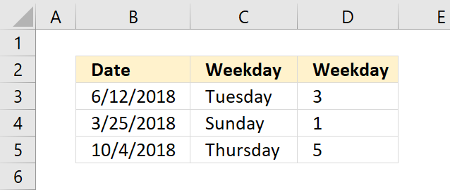
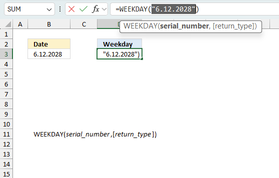
The WEEKDAY function shown in cell D3 in the image above calculates a number based on a date. The number represents a given weekday based on the provided value in the second argument.
The formula below has no second argument, it defaults to 1 meaning the week begins with a Sunday.
Formula in cell D3:
The formula in cell D3 returns 3 which corresponds to a Tuesday if the week starts with a Sunday which corresponds to 1. Number 2 represents Monday. Cell C3 calculates the weekday name and that shows that the date 6/12/2018 is a Tuesday.
Cell B4 contains 3/25/2018, cell C4 shows a "Sunday", and cell D4 returns 1 which corresponds to Sunday if the week starts with a Sunday. As mentioned befroe, the second argument defines when the week begins.
Cell B5 contains 10/4/2018, cell C5 shows "Thursday", and cell D5 returns 5 which corresponds to Thursday if the week starts with a Sunday. 4 is Wednesday, and 5 is Thursday.
4. Function not working
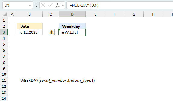
The WEEKDAY function returns
- #VALUE! error if you use an invalid date.
- #NAME? error if you misspell the function name.
- propagates errors, meaning that if the input contains an error (e.g., #VALUE!, #REF!), the function will return the same error.
How do I know the date is recognized as an Excel date?
Check the "Format Cells" dialog box and press with left mouse button on category "General". You should see a number and not a date.
How do I convert a date to an Excel date?
Try using the DATEVALUE function to convert a text date to an Excel date. Read this article if it is not working.
4.1 Troubleshooting the error value
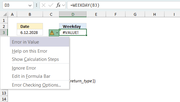
When you encounter an error value in a cell a warning symbol appears, displayed in the image above. Press with mouse on it to see a pop-up menu that lets you get more information about the error.
- The first line describes the error if you press with left mouse button on it.
- The second line opens a pane that explains the error in greater detail.
- The third line takes you to the "Evaluate Formula" tool, a dialog box appears allowing you to examine the formula in greater detail.
- This line lets you ignore the error value meaning the warning icon disappears, however, the error is still in the cell.
- The fifth line lets you edit the formula in the Formula bar.
- The sixth line opens the Excel settings so you can adjust the Error Checking Options.
Here are a few of the most common Excel errors you may encounter.
#NULL error - This error occurs most often if you by mistake use a space character in a formula where it shouldn't be. Excel interprets a space character as an intersection operator. If the ranges don't intersect an #NULL error is returned. The #NULL! error occurs when a formula attempts to calculate the intersection of two ranges that do not actually intersect. This can happen when the wrong range operator is used in the formula, or when the intersection operator (represented by a space character) is used between two ranges that do not overlap. To fix this error double check that the ranges referenced in the formula that use the intersection operator actually have cells in common.
#SPILL error - The #SPILL! error occurs only in version Excel 365 and is caused by a dynamic array being to large, meaning there are cells below and/or to the right that are not empty. This prevents the dynamic array formula expanding into new empty cells.
#DIV/0 error - This error happens if you try to divide a number by 0 (zero) or a value that equates to zero which is not possible mathematically.
#VALUE error - The #VALUE error occurs when a formula has a value that is of the wrong data type. Such as text where a number is expected or when dates are evaluated as text.
#REF error - The #REF error happens when a cell reference is invalid. This can happen if a cell is deleted that is referenced by a formula.
#NAME error - The #NAME error happens if you misspelled a function or a named range.
#NUM error - The #NUM error shows up when you try to use invalid numeric values in formulas, like square root of a negative number.
#N/A error - The #N/A error happens when a value is not available for a formula or found in a given cell range, for example in the VLOOKUP or MATCH functions.
#GETTING_DATA error - The #GETTING_DATA error shows while external sources are loading, this can indicate a delay in fetching the data or that the external source is unavailable right now.
4.2 The formula returns an unexpected value
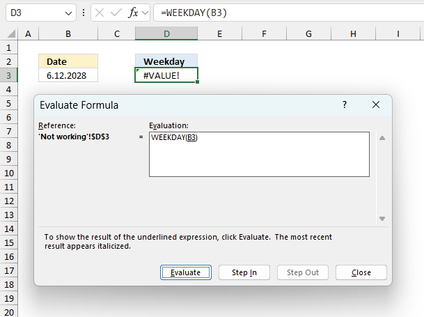
To understand why a formula returns an unexpected value we need to examine the calculations steps in detail. Luckily, Excel has a tool that is really handy in these situations. Here is how to troubleshoot a formula:
- Select the cell containing the formula you want to examine in detail.
- Go to tab “Formulas” on the ribbon.
- Press with left mouse button on "Evaluate Formula" button. A dialog box appears.
The formula appears in a white field inside the dialog box. Underlined expressions are calculations being processed in the next step. The italicized expression is the most recent result. The buttons at the bottom of the dialog box allows you to evaluate the formula in smaller calculations which you control. - Press with left mouse button on the "Evaluate" button located at the bottom of the dialog box to process the underlined expression.
- Repeat pressing the "Evaluate" button until you have seen all calculations step by step. This allows you to examine the formula in greater detail and hopefully find the culprit.
- Press "Close" button to dismiss the dialog box.
There is also another way to debug formulas using the function key F9. F9 is especially useful if you have a feeling that a specific part of the formula is the issue, this makes it faster than the "Evaluate Formula" tool since you don't need to go through all calculations to find the issue.
- Enter Edit mode: Double-press with left mouse button on the cell or press F2 to enter Edit mode for the formula.
- Select part of the formula: Highlight the specific part of the formula you want to evaluate. You can select and evaluate any part of the formula that could work as a standalone formula.
- Press F9: This will calculate and display the result of just that selected portion.
- Evaluate step-by-step: You can select and evaluate different parts of the formula to see intermediate results.
- Check for errors: This allows you to pinpoint which part of a complex formula may be causing an error.
The image above shows cell reference B3 converted to hard-coded value using the F9 key. The WEEKDAY function requires valid Excel dates which is not the case in this example. We have found what is wrong with the formula.
Tips!
- View actual values: Selecting a cell reference and pressing F9 will show the actual values in those cells.
- Exit safely: Press Esc to exit Edit mode without changing the formula. Don't press Enter, as that would replace the formula part with the calculated value.
- Full recalculation: Pressing F9 outside of Edit mode will recalculate all formulas in the workbook.
Remember to be careful not to accidentally overwrite parts of your formula when using F9. Always exit with Esc rather than Enter to preserve the original formula. However, if you make a mistake overwriting the formula it is not the end of the world. You can “undo” the action by pressing keyboard shortcut keys CTRL + z or pressing the “Undo” button
4.3 Other errors
Floating-point arithmetic may give inaccurate results in Excel - Article
Floating-point errors are usually very small, often beyond the 15th decimal place, and in most cases don't affect calculations significantly.
5. Example 2 - show weekday name

The WEEKDAY function returns only a number and not the actual weekday name, however, the TEXT function can do that for you. The TEXT function allows you to format cell values as you prefer, the first argument is value or cell reference. The second argument is the format code you want to use, it provides a wide range of options for customizing the appearance of the cell value.
Formula in cell C3:
The downside using the TEXT function is that you cant perform calculations to the output value since it is a text value. To fix this problem use cell formatting instead. Here is how:
- Select the cell you want to format.
- Press shortcut keys CTRL + 1 (not the plus key). A dialog box appears.
- Go to tab "Number" located on the dialog box if you are not already there.
- You have here a wide range of settings you can choose from. The "Custom" category, in particular, allows you to specify custom format codes, similar to the second argument used in the TEXT function. This gives you a high degree of control over how the cell values are displayed.
- Press with left mouse button on the "OK" button to apply changes and dismiss the dialog box.
Explaining the formula in cell C3
Step 1 - TEXT function
The TEXT function lets you format values. TEXT(value, format_text)
- value - The string you want to format. You can use a cell reference here or use a text string.
- format_text - Formatting code allowing you to change the way, for example, a date or a number is displayed to the Excel user.
Step 2 - Populate arguments
The TEXT function has two arguments.
- value - B3
- format_text - "dddd"
"dddd" returns the weekday. Lower and upper case letters make no difference.
Check out this article to learn more about formatting codes in the TEXT function.
Step 3 - Evaluate TEXT function
TEXT(B3, "dddd") becomes TEXT(43263, "dddd") and returns "Tuesday".

This example shows an entirely different formula that returns the exact same thing as the TEXT function in the example above. The formula calculates the weekday number and uses that to get the correct weekday name from an array. The order of values in the array is very important for this to work.
The weekday number represents the position of the weekday name in the array, the downside with this formula is that it is larger than needed since you need to specify the weekday names and you cant perform calculations to the result.
Formula in cell C4:
The formula in cell C4 returns "Sunday" which is the first value in the array. You need to adjust the formula if you use another value in the second argument in the WEEKDAY function. For example, if you specify an argument that represents a wekk that starts with a Monday instead you also need to rearragne the weekday names in the array so the match a week that begins with a Monday.
Explaining formula
Step 1 - Calculate number representing a weekday
WEEKDAY(B4,1)
becomes
WEEKDAY(43184, 1)
and returns 1.
Step 2 - Return weekday name based on position in array
The INDEX function returns a value in a cell range or array based on a row and column number (optional).
INDEX(array, [row_num], [column_num], [area_num])
INDEX({"Sunday";"Monday";"Tuesday";"Wednesday";"Thursday";"Friday";"Saturday"}, WEEKDAY(B4,1))
becomes
INDEX({"Sunday";"Monday";"Tuesday";"Wednesday";"Thursday";"Friday";"Saturday"}, 1)
and returns "Sunday". "Sunday" is the first value in the array.
6. Example 3 - count days between two given weekdays and two dates

The image above shows an Excel 365 formula that counts days between two dates and also if they are between two given weekdays.
The start date is specified in cell K3, end date is in cell K4. The start weekday is 3 which represents Tuesday, the table in J11:K18 shows the numbers and corresponding weekday names. The end weekday is 5 which represents Thursday.
The calendar in cell range B4:H9 shows which days (bolded) meet the criteria. Cell K9 displays the result, there are six bolded days in the calendar.
Excel 365 dynamic array formula in cell K6:
=LET(x,SEQUENCE(K4-K3+1,,0),y,WEEKDAY(x+K3,1),COUNT(FILTER(x,(y<=K7)*(y>=K6))))
Explaining formula
COUNT(FILTER(SEQUENCE(K4-K3+1,,0),(WEEKDAY(SEQUENCE(K4-K3+1,,0)+K3,1)<=K7)*(WEEKDAY(SEQUENCE(K4-K3+1,,0)+K3,1)>=K6)))
Step 1 - Calculate the number of days and add one
The minus and plus signs let you perform arithmetic operations in an Excel formula
K4-K3+1
44648 - 44631 +1
equals 18.
Step 2 - Create a sequence of numbers from 0 to 18
The SEQUENCE function creates a list of sequential numbers to a cell range or array. It is located in the Math and trigonometry category and is only available to Excel 365 subscribers.
SEQUENCE(rows, [columns], [start], [step])
SEQUENCE(K4-K3+1,,0)
becomes
SEQUENCE(18,,0)
and returns
{0; 1; 2; 3; 4; 5; 6; 7; 8; 9; 10; 11; 12; 13; 14; 15; 16; 17}.
Step 3 - Add date to sequence of numbers
The plus sign lets you perform add numbers in an Excel formula.
SEQUENCE(K4-K3+1,,0)+K3
becomes
{0; 1; 2; 3; 4; 5; 6; 7; 8; 9; 10; 11; 12; 13; 14; 15; 16; 17} + 44631
and returns
{44631; 44632; 44633; 44634; 44635; 44636; 44637; 44638; 44639; 44640; 44641; 44642; 44643; 44644; 44645; 44646; 44647; 44648}.
Step 4 - Calculate weekday
WEEKDAY(SEQUENCE(K4-K3+1,,0)+K3,1)
becomes
WEEKDAY({44631; 44632; 44633; 44634; 44635; 44636; 44637; 44638; 44639; 44640; 44641; 44642; 44643; 44644; 44645; 44646; 44647; 44648},1)
and returns
{6; 7; 1; 2; 3; 4; 5; 6; 7; 1; 2; 3; 4; 5; 6; 7; 1; 2}.
Step 5 - Check if number is less than seven
The less than and larger than characters let you check if a value is smaller or larger than a condition, the result is a boolean value TRUE or FALSE. The equal sign and the less than character combined compare if values are equal or smaller than a condition.
WEEKDAY(SEQUENCE(K4-K3+1,,0)+K3,1)<=K7
becomes
{6; 7; 1; 2; 3; 4; 5; 6; 7; 1; 2; 3; 4; 5; 6; 7; 1; 2}<=5
and returns
{FALSE; FALSE; TRUE; TRUE; TRUE; TRUE; TRUE; FALSE; FALSE; TRUE; TRUE; TRUE; TRUE; TRUE; FALSE; FALSE; TRUE; TRUE}.
Step 6 - Check if weekday is larger than one
WEEKDAY(SEQUENCE(K4-K3+1,,0)+K3,1)>=K6
becomes
{6; 7; 1; 2; 3; 4; 5; 6; 7; 1; 2; 3; 4; 5; 6; 7; 1; 2}>=3
and returns
{TRUE; TRUE; FALSE; FALSE; TRUE; TRUE; TRUE; TRUE; TRUE; FALSE; FALSE; TRUE; TRUE; TRUE; TRUE; TRUE; FALSE; FALSE}.
Step 7 - Multiply arrays
The asterisk character lets you multiple values in an Excel formula. Multiplying boolean values always return their numerical equivalents.
TRUE -> 1
FALSE -> 0 (zero)
(WEEKDAY(SEQUENCE(K4-K3+1,,0)+K3,1)<7)*(WEEKDAY(SEQUENCE(K4-K3+1,,0)+K3,1)>1)
becomes
{FALSE; FALSE; TRUE; TRUE; TRUE; TRUE; TRUE; FALSE; FALSE; TRUE; TRUE; TRUE; TRUE; TRUE; FALSE; FALSE; TRUE; TRUE}*{TRUE; TRUE; FALSE; FALSE; TRUE; TRUE; TRUE; TRUE; TRUE; FALSE; FALSE; TRUE; TRUE; TRUE; TRUE; TRUE; FALSE; FALSE}
and returns
{0; 0; 0; 0; 1; 1; 1; 0; 0; 0; 0; 1; 1; 1; 0; 0; 0; 0}.
Step 8 - Filter numbers based on condition
The FILTER function is a new function available to Excel 365 subscribers. It lets you extract values based on a condition or criteria.
FILTER(array, include, [if_empty])
FILTER(SEQUENCE(K4-K3+1,,0),(WEEKDAY(SEQUENCE(K4-K3+1,,0)+K3,1)<7)*(WEEKDAY(SEQUENCE(K4-K3+1,,0)+K3,1)>1))
becomes
FILTER({0; 1; 2; 3; 4; 5; 6; 7; 8; 9; 10; 11; 12; 13; 14; 15; 16; 17},{0; 0; 0; 0; 1; 1; 1; 0; 0; 0; 0; 1; 1; 1; 0; 0; 0; 0})
and returns
{4; 5; 6; 11; 12; 13}.
Step 9 - Count numbers in the array
The COUNT function counts all numbers in a cell range or array.
COUNT(value1, [value2], ...)
COUNT(FILTER(SEQUENCE(K4-K3+1,,0),(WEEKDAY(SEQUENCE(K4-K3+1,,0)+K3,1)<7)*(WEEKDAY(SEQUENCE(K4-K3+1,,0)+K3,1)>1)))
becomes
COUNT({4; 5; 6; 11; 12; 13})
and returns 6. There are six numbers in the array.
Step 10 - Shorten formula
The LET function allows you to name intermediate calculation results which can shorten formulas considerably and improve performance.
LET(name1, name_value1, calculation_or_name2, [name_value2, calculation_or_name3...])
LET(x, SEQUENCE(K4-K3+1, , 0), y, WEEKDAY(x+K3, 1), COUNT(FILTER(x, (y<7)*(y>1))))
x - SEQUENCE(K4-K3+1,,0)
y - WEEKDAY(x+K3,1)
7. Example 4 - how to calculate a date based on specific weekday in a month
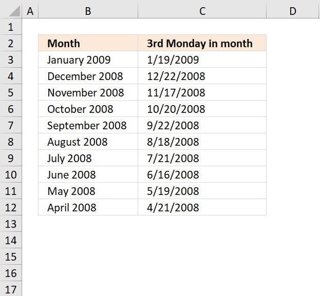
Question: How to calculate the date of the third Monday of a given month?
Answer: Column B contains dates of the first date of a month in the image above, however, they are formatted as Month and year. This makes it possible to use the corresponding cell value in our formula.
Cell range C3:C12 contains the result, they calculate the date of the third Monday in the given month specified on the same row in column B.
The following formulas calculates the same thing, the first one works only in Excel 365 and the next one works also in previous versions.
Excel 365 dynamic array formula in cell C3:
Excel 365 dynamic arrays spill to adjacent cells a s far as needed, in this case, to cells below. Note that this formula is entered as a regular formula and the formula below as an array formula.
Array formula in cell C3:
To enter an array formula, type the formula in cell C3 then press and hold CTRL + SHIFT simultaneously, now press Enter once. Release all keys.
 The formula bar now shows the formula with a beginning and ending curly bracket telling you that you entered the formula successfully.
Don't enter the curly brackets yourself, they appear automatically.
Explaining array formula in cell C3
Step 1 - Create an array of numbers corresponding to days in month
The EOMONTH function calculates the last date in a given month, the DAY function then returns the day of that date.
ROW(INDIRECT( "$1:$"&DAY( EOMONTH(B3, 0))))-1)
becomes
ROW(INDIRECT( "$1:$"&DAY( EOMONTH(39814, 0))))-1)
becomes
ROW(INDIRECT( "$1:$"&DAY( 39844)))-1)
becomes
ROW(INDIRECT( "$1:$"&DAY( 39844)))-1)
becomes
ROW(INDIRECT("$1:$"&31))-1
The INDIRECT function converts a text string to a cell reference that an Excel function then can use.
ROW(INDIRECT($1:$31))-1
becomes
ROW($1:$31)-1
The ROW function then returns the row numbers of each cell in the cell reference.
ROW($1:$31)-1
becomes
{1; 2; 3; 4; 5; 6; 7; 8; 9; 10; 11; 12; 13; 14; 15; 16; 17; 18; 19; 20; 21; 22; 23; 24; 25; 26; 27; 28; 29; 30; 31} - 1
and returns {0; 1; 2; 3; 4; 5; 6; 7; 8; 9; 10; 11; 12; 13; 14; 15; 16; 17; 18; 19; 20; 21; 22; 23; 24; 25; 26; 27; 28; 29; 30}
Step 2 - Check if date is a Monday
The array in the step before is now going to be added to the first date in the given month.
WEEKDAY(B3 +ROW(INDIRECT( "$1:$"&DAY( EOMONTH(B3, 0))))-1)=2
becomes
WEEKDAY(B3 +{0; 1; 2; 3; 4; 5; 6; 7; 8; 9; 10; 11; 12; 13; 14; 15; 16; 17; 18; 19; 20; 21; 22; 23; 24; 25; 26; 27; 28; 29; 30})=2
becomes
WEEKDAY({39814; 39815; 39816; 39817; 39818; 39819; 39820; 39821; 39822; 39823; 39824; 39825; 39826; 39827; 39828; 39829; 39830; 39831; 39832; 39833; 39834; 39835; 39836; 39837; 39838; 39839; 39840; 39841; 39842; 39843; 39844})=2
It is worth mentioning that Excel treats dates as numbers. For example, number 1 is 1/1/1900 and 1/1/2000 is 36526. 1/2/2000 is 36527. The numbers you see above in the array are dates.
The WEEKDAY function converts the dates to their corresponding weekdays in numbers. 1 is Sunday and 7 is Saturday.
WEEKDAY({39814; 39815; 39816; 39817; 39818; 39819; 39820; 39821; 39822; 39823; 39824; 39825; 39826; 39827; 39828; 39829; 39830; 39831; 39832; 39833; 39834; 39835; 39836; 39837; 39838; 39839; 39840; 39841; 39842; 39843; 39844})=2
becomes
{5;6;7;1;2;3;4;5;6;7;1;2;3;4;5;6;7;1;2;3;4;5;6;7;1;2;3;4;5;6;7}=2
To identify Mondays in this array I will compare the numbers with 2.
{5;6;7;1;2;3;4;5;6;7;1;2;3;4;5;6;7;1;2;3;4;5;6;7;1;2;3;4;5;6;7}=2
returns the following boolean array:
{FALSE; FALSE; FALSE; FALSE; TRUE; FALSE; FALSE; FALSE; FALSE; FALSE; FALSE; TRUE; FALSE; FALSE; FALSE; FALSE; FALSE; FALSE; TRUE; FALSE; FALSE; FALSE; FALSE; FALSE; FALSE; TRUE; FALSE; FALSE; FALSE; FALSE; FALSE}
Boolean values are TRUE and FALSE.
Step 3 - Return corresponding date if Monday
The IF function lets you evaluate a logical expression and if TRUE one thing happens and if FALSE another thing happens.
The logical expression in this example evaluates to TRUE if date is a Monday.
IF(WEEKDAY(B3+ROW(INDIRECT("$1:$"&DAY(EOMONTH(B3,0))))-1)=2,B3+ROW(INDIRECT("$1:$"&DAY(EOMONTH(B3,0))))-1,"")
becomes
IF({FALSE; FALSE; FALSE; FALSE; TRUE; FALSE; FALSE; FALSE; FALSE; FALSE; FALSE; TRUE; FALSE; FALSE; FALSE; FALSE; FALSE; FALSE; TRUE; FALSE; FALSE; FALSE; FALSE; FALSE; FALSE; TRUE; FALSE; FALSE; FALSE; FALSE; FALSE},B3+ROW(INDIRECT("$1:$"&DAY(EOMONTH(B3,0))))-1,"")
If the value is TRUE then return the corresponding date. Since months have different number of days we must build an array that takes that into account.
It works just like the array we created in step 1.
IF({FALSE; FALSE; FALSE; FALSE; TRUE; FALSE; FALSE; FALSE; FALSE; FALSE; FALSE; TRUE; FALSE; FALSE; FALSE; FALSE; FALSE; FALSE; TRUE; FALSE; FALSE; FALSE; FALSE; FALSE; FALSE; TRUE; FALSE; FALSE; FALSE; FALSE; FALSE},B3+ROW(INDIRECT("$1:$"&DAY(EOMONTH(B3,0))))-1,"")
becomes
IF({FALSE; FALSE; FALSE; FALSE; TRUE; FALSE; FALSE; FALSE; FALSE; FALSE; FALSE; TRUE; FALSE; FALSE; FALSE; FALSE; FALSE; FALSE; TRUE; FALSE; FALSE; FALSE; FALSE; FALSE; FALSE; TRUE; FALSE; FALSE; FALSE; FALSE; FALSE},{39814; 39815; 39816; 39817; 39818; 39819; 39820; 39821; 39822; 39823; 39824; 39825; 39826; 39827; 39828; 39829; 39830; 39831; 39832; 39833; 39834; 39835; 39836; 39837; 39838; 39839; 39840; 39841; 39842; 39843; 39844},"")
and returns
{""; ""; ""; ""; 39818; ""; ""; ""; ""; ""; ""; 39825; ""; ""; ""; ""; ""; ""; 39832; ""; ""; ""; ""; ""; ""; 39839; ""; ""; ""; ""; ""}
Step 3 - Filter third Monday
The SMALL function lets you return the third largest number in array because we are looking for the third Monday in a given month.
SMALL(IF(WEEKDAY(B3 +ROW(INDIRECT( "$1:$"&DAY( EOMONTH(B3, 0))))-1)=2, B3+ROW( INDIRECT("$1:$"&DAY( EOMONTH(B3, 0))))-1, ""), 3)
becomes
SMALL({""; ""; ""; ""; 39818; ""; ""; ""; ""; ""; ""; 39825; ""; ""; ""; ""; ""; ""; 39832; ""; ""; ""; ""; ""; ""; 39839; ""; ""; ""; ""; ""}, 3)
and returns 39832 in cell C3 which is the same as 1/19/2009 if formatted as a date in Excel.
Get Excel *.xlsx file
'WEEKDAY' function examples
This article explains how to calculate an overlapping time ranges across multiple days. This can be very useful in situations […]
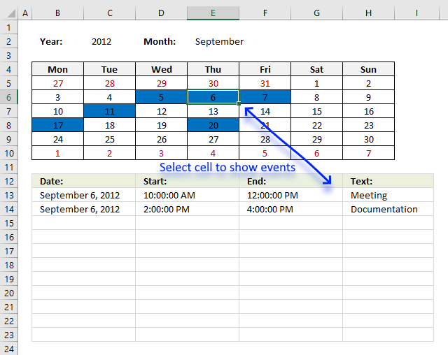
Table of Contents Excel monthly calendar - VBA Calendar Drop down lists Headers Calculating dates (formula) Conditional formatting Today Dates […]
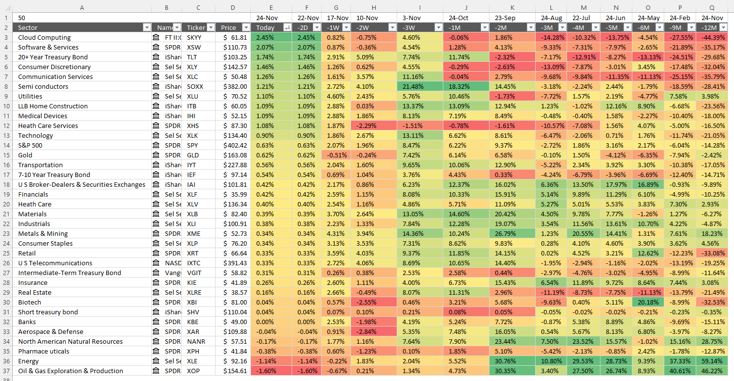
The image above shows the performance across industry groups for different date ranges, conditional formatting makes the table much easier […]
Functions in 'Date and Time' category
The WEEKDAY function function is one of 22 functions in the 'Date and Time' category.
How to comment
How to add a formula to your comment
<code>Insert your formula here.</code>
Convert less than and larger than signs
Use html character entities instead of less than and larger than signs.
< becomes < and > becomes >
How to add VBA code to your comment
[vb 1="vbnet" language=","]
Put your VBA code here.
[/vb]
How to add a picture to your comment:
Upload picture to postimage.org or imgur
Paste image link to your comment.
Contact Oscar
You can contact me through this contact form