How to track sector performance in the stock market – Excel template

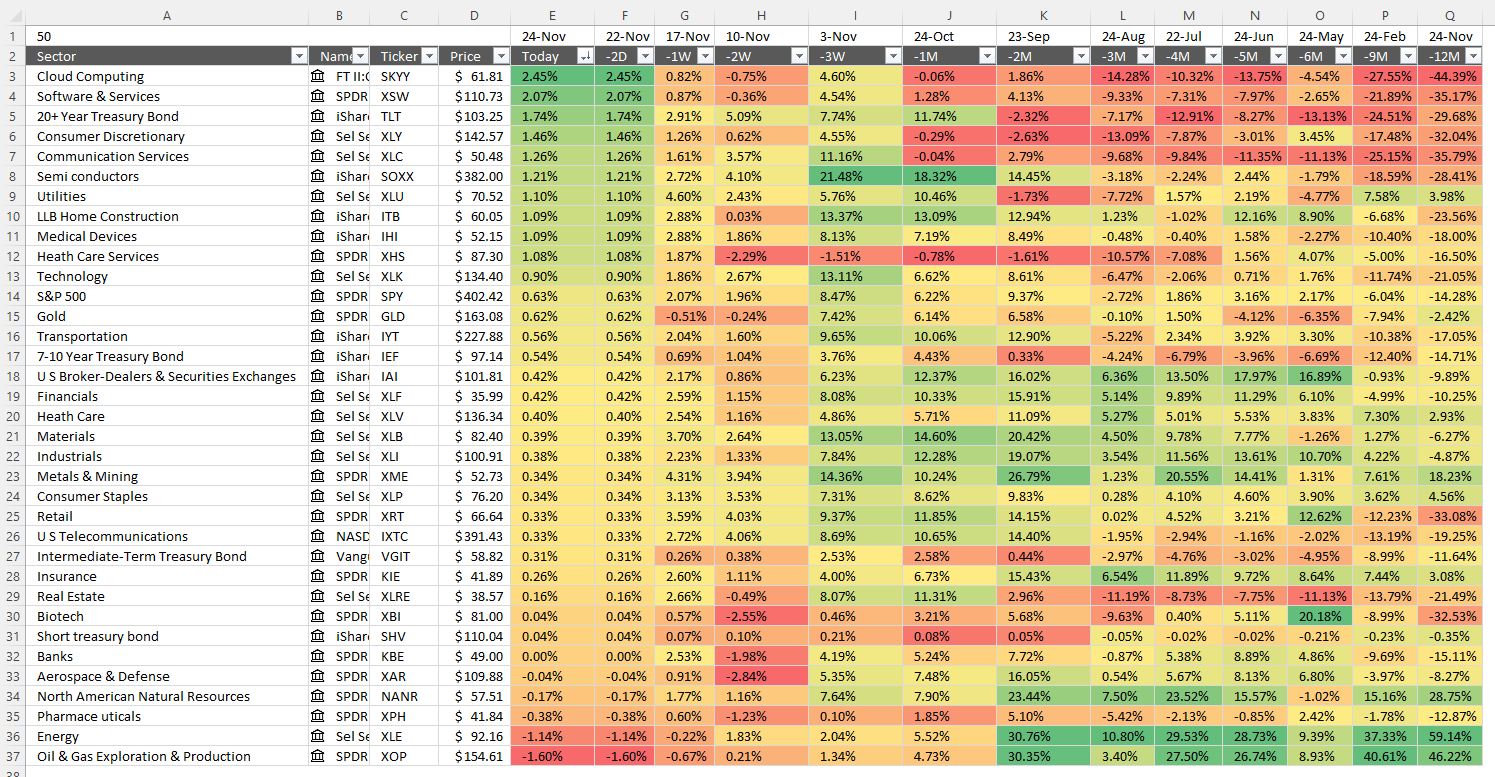
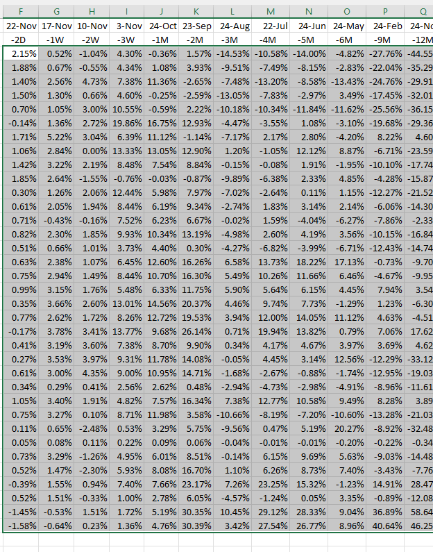
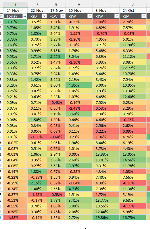
The image above shows the performance across industry groups for different date ranges, conditional formatting makes the table much easier to read. Press with left mouse button on the image to see a larger version.

I will in this post demonstrate how I built it and there is also a link to the workbook. The worksheet is easy to customize, you can add individual stocks och indexes that you find interesting.

The whole table refreshes automatically no need to adjust anything, however, Excel 365 is needed. The STOCKHISTORY function is used in order to fetch historical stock prices.

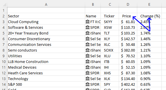
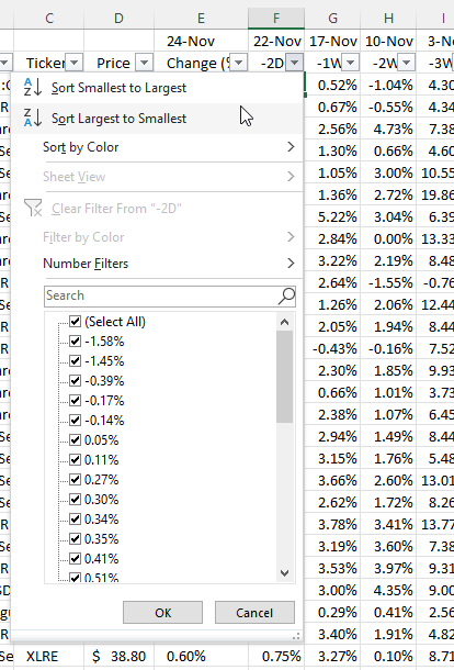
There are arrows next to each column header allowing you to sort the column you find most interesting.

1. Introduction

• Why track sector performance?
  Every new bull market (a growing economy) has one or a few more sectors that advances quicker than the remaining sectors. You want to own the best performing stocks in these leading sectors. The table above lets you identify these sectors when the market turns up.
• What is a sector?
  A sector refers to a group of companies that operate in the same industry or have similar business activities. The stock market is divided into sectors to help categorize businesses and investments. Examples of sectors include Technology, Healthcare, Finance, Energy, Consumer Goods, and Industrials.
• What is a stock market?
  The stock market is a marketplace where investors buy and sell stocks (shares of ownership in companies). It includes stock exchanges like the New York Stock Exchange (NYSE), Nasdaq, London Stock Exchange (LSE), and Tokyo Stock Exchange (TSE). The stock market allows companies to raise capital and provides investors with opportunities to profit from stock price movements.
  
• What is a stock?
  A stock represents ownership in a company. When you buy a stock, you own a small part of that company, known as a share. Stocks can be classified into:
  • Common stocks – Give voting rights and potential dividends.
  • Preferred stocks – Usually offer fixed dividends but limited voting rights.
• What is a stock symbol?
  A stock symbol (ticker symbol) is a unique abbreviation used to identify a publicly traded company on a stock exchange. It consists of letters or a combination of letters and numbers. Examples:
  • AAPL – Apple Inc. (Nasdaq)
  • TSLA – Tesla, Inc. (Nasdaq)
  • GOOGL – Alphabet Inc. (Nasdaq)
  • MSFT – Microsoft Corporation (Nasdaq)
    Stock symbols help investors and traders quickly find and track company stocks.
• What is a bull market?
  A bull market refers to a period of rising stock prices, typically by 20% or more after a previous decline. It signals strong investor confidence, economic growth, and increasing demand for stocks. Bull markets can last for months or even years.
• What is a bear market?
  A bear market is a period of declining stock prices, typically defined as a 20% or more drop from recent highs. It is associated with negative investor sentiment, economic slowdown, and reduced market confidence. Bear markets can last for weeks, months, or even years.
• What is the stock data type?
  In Microsoft Excel, the Stock data type allows users to retrieve real-time stock market data from the internet. It includes details like ticker symbols, company names, latest prices, 52-week highs/lows, market capitalization, and more. You can convert a stock symbol into this data type by selecting it and choosing "Stocks" from the Data tab in Excel.
• What is conditional formatting?
  Conditional formatting in Excel (and other spreadsheet software) is a feature that applies automatic formatting (such as color changes, bold text, or icons) to cells based on certain conditions or rules. For example:
  • Highlighting all sales above $10,000 in green.
  • Making negative numbers appear in red.
  • Applying a color gradient based on value ranges.
• What is an Excel 365 dynamic array formula?
  A dynamic array formula in Excel 365 is a formula that automatically "spills" results into multiple cells based on available data. Unlike traditional formulas, dynamic arrays resize automatically when data changes.
• How do I enter an Excel 365 dynamic array formula?
  To enter a dynamic array formula in Excel 365:
  • Select a single cell where you want the results to start.
  • Type your formula.
  • Press Enter (no need to press Ctrl+Shift+Enter as in older versions).
  • Excel will "spill" the results into multiple cells automatically.
• What is Autofilter in Excel?
  Autofilter in Excel is a feature that allows you to filter and sort data quickly based on specific criteria. It is commonly used to display only the rows that meet certain conditions while hiding the rest.

2. Add sectors, names, and tickers to the worksheet

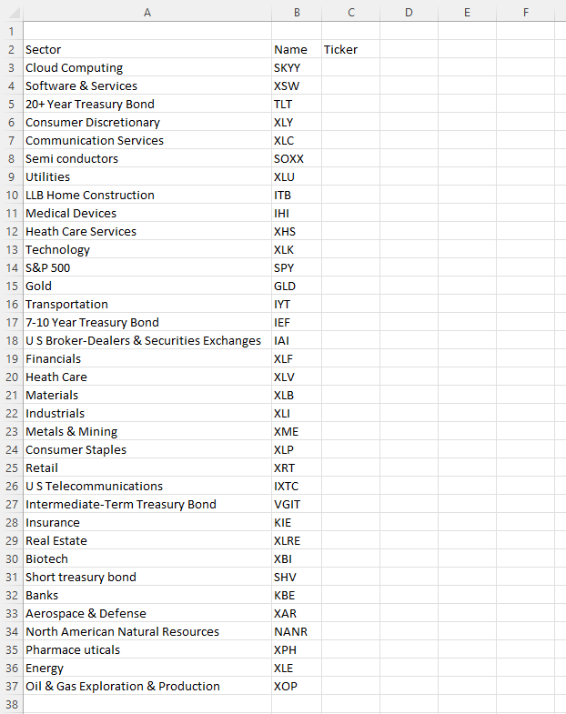
Column A contains names of ETFs that track a sector, column B the corresponding ticker.

Select all tickers in column B.

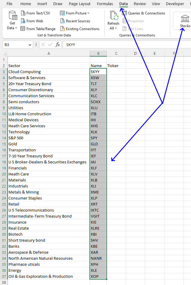
Go to tab "Data" on the ribbon.

Press with left mouse button on "Stocks" button, see the image above.

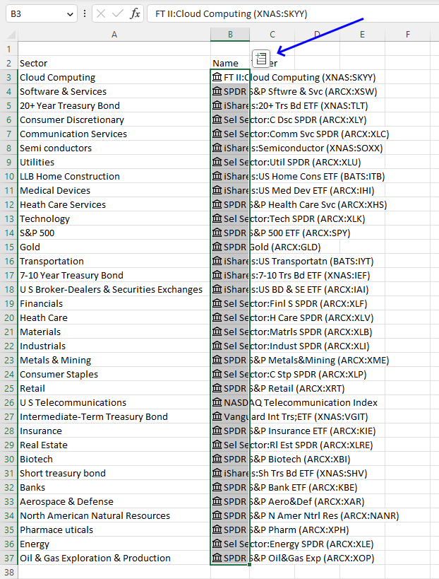
The tickers change and a "stock" icon appears next to the name in column B. A new button appears, see the image above.

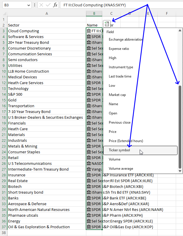
Press with left mouse button on the button, a popup drop-down list appears.

Scroll down until you see "Ticker symbol", press with left mouse button on the "Ticker Symbol". See the image above.

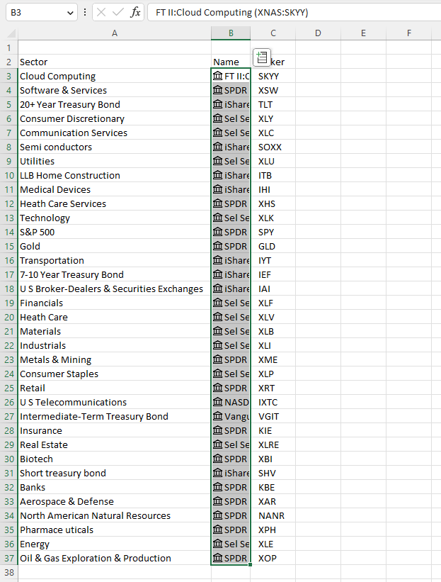
The table expands to the right, tickers are now visible in column C.

Press with left mouse button on the button again to see the popup drop-down list, press with left mouse button on "Price", and see the image below.

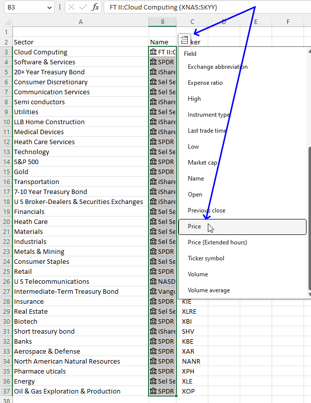
The table expands once again, current prices are now shown, or at least the last price. We will use the price value and the STOCKHISTORY function to calculate performance later in this article in section 3.

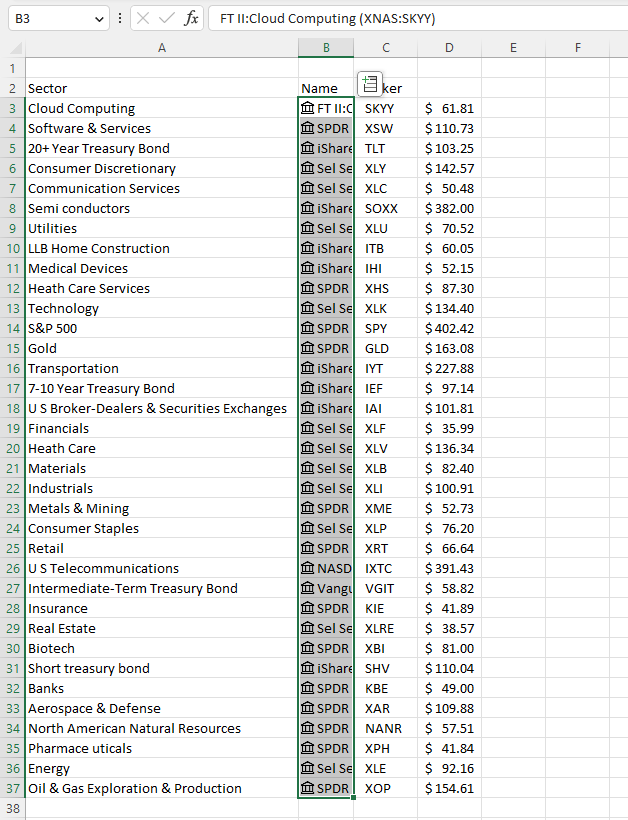
Press with left mouse button on the button again and now select "Change (%)".

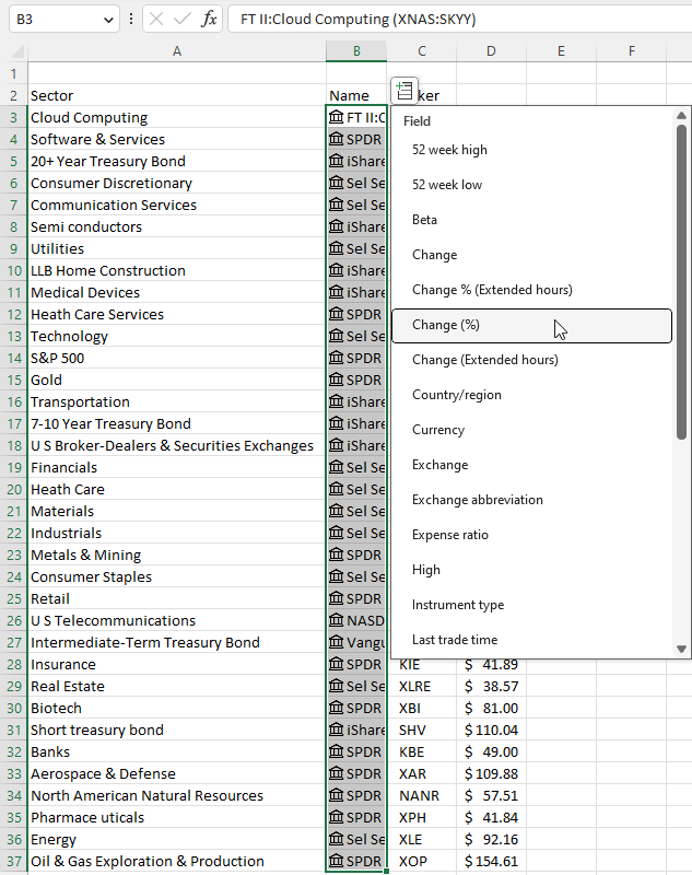
A new column (E) appears showing the change in percent, see the image below. The percentage shows how the sector is doing right now if the stock market is open.

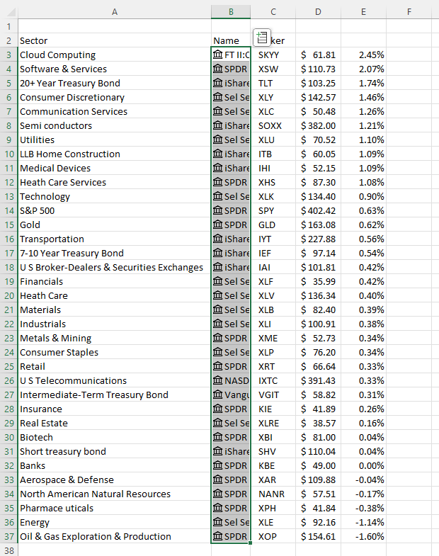
Add column header names for "Price" and "Change (%)".

Back to top

2. Calculate dates for each date range

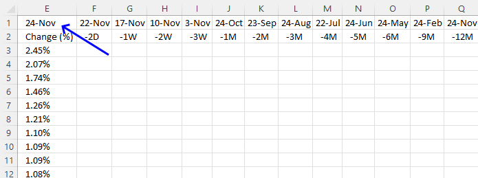
Cell E1 contains a formula that returns the current date, this formula is volatile meaning it recalculates more often than non-volatile functions.

Formula in cell E1:

The TODAY function returns the Excel date (serial number) of the current date.

Function syntax: TODAY()

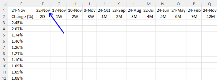
Cell F1 calculates the date two workdays earlier, this formula is also volatile since it references cell E1.

Formula in cell F1:

The WORKDAY function returns a date based on a start date and a given number of working days (nonweekend and nonholidays).

Function syntax: WORKDAY(start_date, days, [holidays])

Table1[Holidays] is a reference to a column in an Excel defined Table.

I recommend adding holidays to this formula to prevent dates when the stock market is closed.

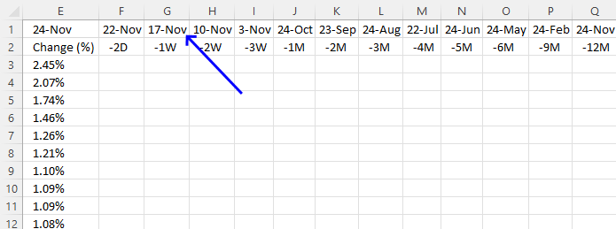
Cell G1 returns a date one week earlier than the date in cell E1.

Formula in cell G1:

The WORKDAY function returns a date based on a start date and a given number of working days (nonweekend and nonholidays).

Function syntax: WORKDAY(start_date, days, [holidays])

I recommend adding holidays to this formula to prevent dates when the stock market is closed.

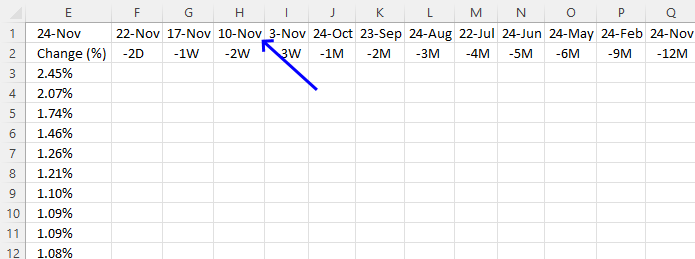
Cell H1 returns a date two weeks earlier than the date in cell E1.

Formula in cell H1:

The WORKDAY function returns a date based on a start date and a given number of working days (nonweekend and nonholidays).

Function syntax: WORKDAY(start_date, days, [holidays])

I recommend adding holidays to this formula to prevent dates when the stock market is closed.

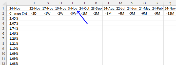
Cell I1 returns a date three weeks earlier than the date in cell E1.

Formula in cell I1:

The WORKDAY function returns a date based on a start date and a given number of working days (nonweekend and nonholidays).

Function syntax: WORKDAY(start_date, days, [holidays])

I recommend adding holidays to this formula to prevent dates when the stock market is closed.

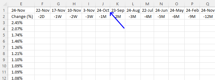
This formula calculates a date one month earlier than the date in cell E1 and makes sure the date is not a Saturday or Sunday. I recommend adding holidays to the WORKDAY function to prevent dates when the stock market is closed.

Formula in cell J1:

2.1 Explaining formula

Step 1 - Calculate the year based on an Excel date

The YEAR function converts a date to a number representing the year in the date.

Function syntax: YEAR(serial_number)

YEAR($E$1)

becomes

YEAR(44887)

and returns 2022.

Step 2 - Calculate the month

The MONTH function extracts the month as a number from an Excel date.

Function syntax: MONTH(serial_number)

MONTH($E$1)-1

The minus character lets you subtract numbers in an Excel formula. This allows us to calculate the month before.

MONTH($E$1)-1

becomes

MONTH(44887)-1

becomes

11-1

and returns 10.

Step 3 - Calculate the day

The DAY function extracts the day as a number from an Excel date.

Function syntax: DAY(serial_number)

DAY($E$1)

becomes

DAY(44887)

and returns 22.

Step 4 - Create an Excel date based on year, month, and day values

The DATE function returns a number that acts as a date in the Excel environment.

Function syntax: DATE(year, month, day)

DATE(YEAR($E$1),MONTH($E$1)-1,DAY($E$1))

becomes

DATE(2022, 10, 22)

and returns

44856.

Step 5 - Calculate weekday number

The WEEKDAY function converts a date to a weekday number from 1 to 7.

Function syntax: WEEKDAY(serial_number,[return_type])

WEEKDAY(DATE(YEAR($E$1),MONTH($E$1)-1,DAY($E$1)),2)

becomes

WEEKDAY(44856,2)

and returns 6.

Step 6 - Identify Saturdays and Sundays

The larger than and smaller than characters lets you compare number to number, the result is a boolean value TRUE or FALSE.

A value larger than 5 tells us that the date is a Saturday or Sunday.

WEEKDAY(DATE(YEAR($E$1),MONTH($E$1)-1,DAY($E$1)),2)>5

becomes

6>5

and returns TRUE.

Step 7 - Check if the date is a holiday

The equal sign lets you check if a value is equal to another value, and the result is a boolean value TRUE or FALSE.

DATE(YEAR($E$1),MONTH($E$1)-1,DAY($E$1))=Table1[Holidays]

becomes

44856={44746; 44525; 44889}

and returns

{FALSE; FALSE; FALSE}

10/22/2022 is not in the list of holidays.

Step 8 - Check if at least one of the boolean values is equal to TRUE

The OR function evaluates a logical expression in each argument and if at least one argument returns TRUE the OR function returns TRUE. If all arguments return FALSE the OR function also returns FALSE.

Function syntax: OR(logical1, [logical2])

OR(DATE(YEAR($E$1),MONTH($E$1)-1,DAY($E$1))=Table1[Holidays]))

becomes

OR({FALSE; FALSE; FALSE})

and returns

FALSE.

Step 9 - Check if at least one of the boolean values is equal to TRUE

The OR function evaluates a logical expression in each argument and if at least one argument returns TRUE the OR function returns TRUE. If all arguments return FALSE the OR function also returns FALSE.

Function syntax: OR(logical1, [logical2])

OR(WEEKDAY(DATE(YEAR($E$1),MONTH($E$1)-1,DAY($E$1)),2)>5,OR(DATE(YEAR($E$1),MONTH($E$1)-1,DAY($E$1))=Table1[Holidays]))

becomes

OR(TRUE, FALSE)

and returns

TRUE.

Step 10 - Calculate the workday date one day back

The WORKDAY function returns a date based on a start date and a given number of working days (nonweekend and nonholidays).

Function syntax: WORKDAY(start_date, days, [holidays])

WORKDAY(DATE(YEAR($E$1),MONTH($E$1)-1,DAY($E$1)),-1,,Table1[Holidays])

becomes

WORKDAY(44856,-1)

and returns

44854.

Step 11 - Check if the date is a weekend or a holiday

The IF function returns one value if the logical test is TRUE and another value if the logical test is FALSE.

Function syntax: IF(logical_test, [value_if_true], [value_if_false])

This IF function checks if the date is a weekend or a holiday specified in Table1[Holidays]. If true then return the first earlier workday, if not true then show the date.

IF(OR(WEEKDAY(DATE(YEAR($E$1),MONTH($E$1)-1,DAY($E$1)),2)>5,OR(DATE(YEAR($E$1),MONTH($E$1)-1,DAY($E$1))=Table1[Holidays])),WORKDAY(DATE(YEAR($E$1),MONTH($E$1)-1,DAY($E$1)),-1,Table1[Holidays]),DATE(YEAR($E$1),MONTH($E$1)-1,DAY($E$1)))

becomes

IF(TRUE, 44854, 44856)

and returns

44854

Step 12 - Shorten the formula

The LET function lets you name intermediate calculation results which can shorten formulas considerably and improve performance.

Function syntax: LET(name1, name_value1, calculation_or_name2, [name_value2, calculation_or_name3...])

IF(OR(WEEKDAY(DATE(YEAR($E$1),MONTH($E$1)-1,DAY($E$1)),2)>5,OR(DATE(YEAR($E$1),MONTH($E$1)-1,DAY($E$1))=Table1[Holidays])),WORKDAY(DATE(YEAR($E$1),MONTH($E$1)-1,DAY($E$1)),-1,Table1[Holidays]),DATE(YEAR($E$1),MONTH($E$1)-1,DAY($E$1)))

y - $E$1

x - DATE(YEAR(y),MONTH(y)-1,DAY(y))

LET(y,$E$1,x,DATE(YEAR(y),MONTH(y)-1,DAY(y)),IF(OR(WEEKDAY(x,2)>5,OR(x=Table1[Holidays])),WORKDAY(x,-1,,Table1[Holidays]),x))

Back to top

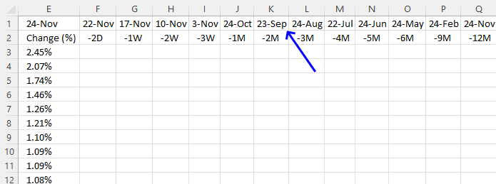
This formula is the same as in cell J1 with one minor exception, it subtracts by two instead of one.

Formula in cell K1:

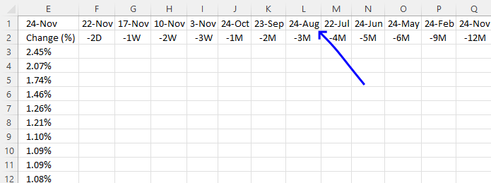
This formula is the same as in cell J1 with one minor exception, it subtracts by three instead of one.

Formula in cell L1:

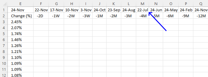
This formula is the same as in cell J1 with one minor exception, it subtracts by four instead of one.

Formula in cell M1:

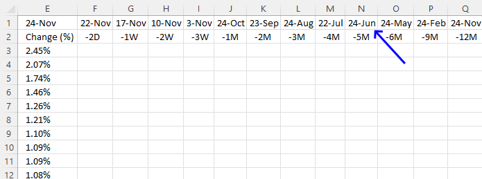
This formula is the same as in cell J1 with one minor exception, it subtracts by five instead of one.

Formula in cell N1:

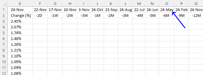
This formula is the same as in cell J1 with one minor exception, it subtracts by six instead of one.

Formula in cell O1:

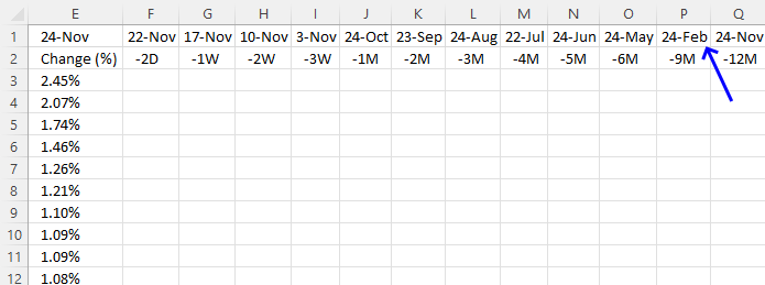
This formula is the same as in cell J1 with one minor exception, it subtracts by nine instead of one.

Formula in cell P1:

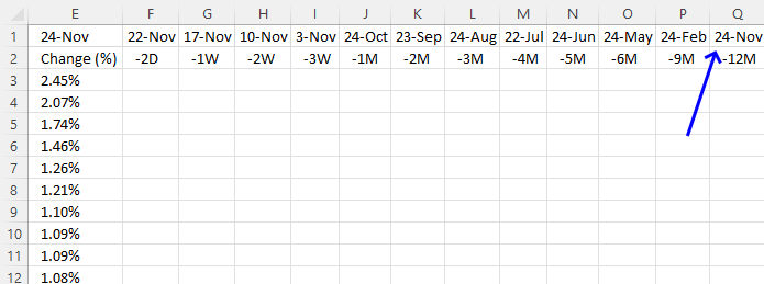
This formula is the same as in cell J1 with one minor exception, it subtracts by twelve instead of one.

Formula in cell Q1:

Back to top

3. Get historical stock prices based on ticker/symbol and date range

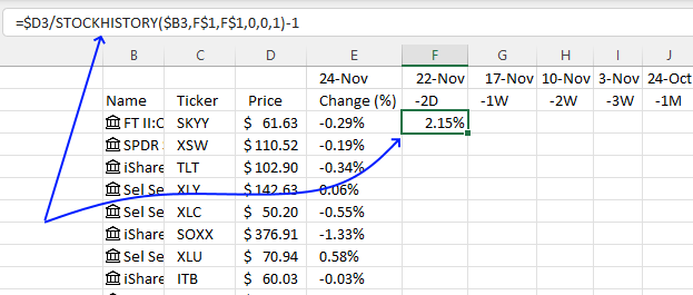
This formula calculates the change or percentage of a specific sector between today and a date in the past. This allows us to monitor change across days, weeks, months and years. We will utilize conditional formatting in section 6 to further visualize the change, in other words the cell color will help us easily spot growing and declining sectors.

Formula in cell F3:

3.1 Explaining formula

Step 1 - Get the closing stock price value for a given date

The STOCKHISTORY function downloads stock prices based on a stock quote

Function syntax: STOCKHISTORY(stock, start_date, [end_date], [interval], [headers], [property0], [property1], [property2], [property3], [property4], [property5])

STOCKHISTORY($B3,F$1,F$1,0,0,1)

Cell reference $B3 is "locked" to column B and cell references F$1 are locked to row 1. This will change the cell references appropriately as we copy the cell and paste it to adjacent cells.

STOCKHISTORY($B3,F$1,F$1,0,0,1)

becomes

STOCKHISTORY("SKYY", 44887, 44887,0,0,1)

and returns

60.33

Step 2 - Divide latest stock price value by historical stock price value

The division character lets you divide numbers in an Excel formula.

$D3/STOCKHISTORY($B3,F$1,F$1,0,0,1)

becomes

61.63/60.33

and returns

1.02154815183159

Step 3 - Subtract the result by 1

The minus character lets you subtract numbers in an Excel formula. This allows us to calculate the percentage even if the stock price is declining.

$D3/STOCKHISTORY($B3,F$1,F$1,0,0,1)-1

becomes

1.02154815183159 - 1

and returns

0.021548151831593

Back to top

3.2 How to format a cell showing a percentage

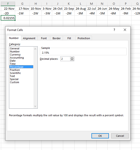
1. Select cell F3
2. Press CTRL + 1 to open the "Format Cells" dialog box.
3. Press with left mouse button on "Percentage".
4. Press with left mouse button on "OK" button to apply changes.

Back to top

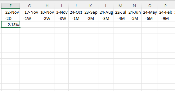
3.3 Copy cell and paste to adjacent cells

1. Select cell F3.
2. Press CTRL + c to copy the cell.
3. Select cell range F3:Q37.
4. Press CTRL + v to paste the formula.

Back to top

4. Enable Autofilter

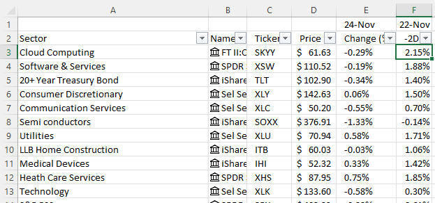
The AutoFilter feature in Excel allows us to sort the sectors based on a specific condition. The small boxes next to the column header names indicates that AutoFilter is applied to the data set. Press with mouse one of the boxes to sort, or apply a condition to that particular column. For example:

• Sort by sector name
• Sort by ticker or symbol
• Sort by price
• Sort by change
  • day
  • week
  • month
  • year

Here is how to apply the AutoFilter tool in Excel:

1. Select any cell in the table.
2. Go to tab "Data" on the ribbon.
   
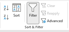
3. Press with left mouse button on the "Filter" button.

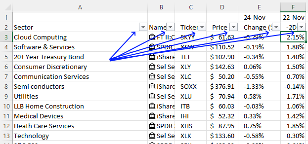
Buttons next to header names appear, they let you sort the table.

Back to top

5. Apply conditional formatting

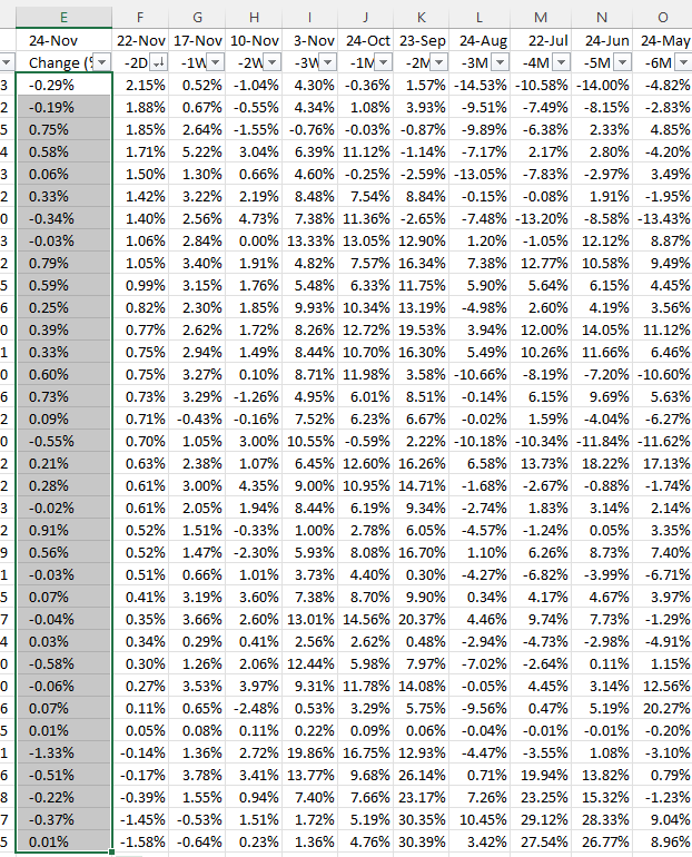
Conditional formatting allows for highlighting significant sector performance advances or declines, meaning you can easily spot sectors that are growing or declining based on cell color. Here is how to apply conditional formatting:

1. Select cell range E3:E37.
2. Go to tab "Home" on the ribbon.
   
3. Press with left mouse button on the "Conditional Formatting" button.
   
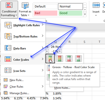
4. Press with left mouse button on "Color Scales".
5. Press with left mouse button on the "Green - Yellow - Red Color Scale"
   
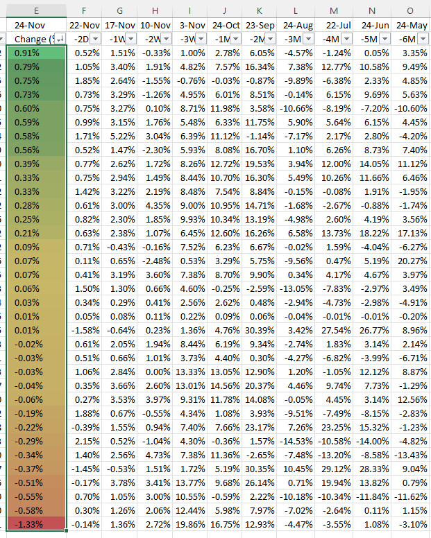
6. Copy cell range E3:E37.
7. Select cell range F3:F37.
8. Press with right mouse button on on the selected cell range.
   
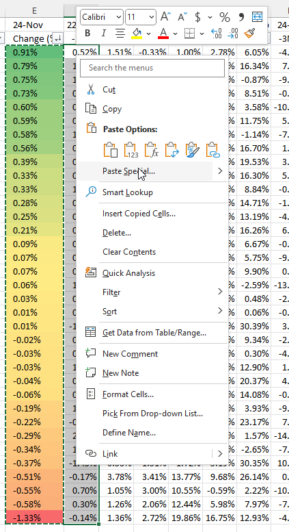
9. Select "Paste Special...", a dialog box appears.
   
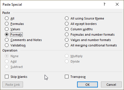
10. Press with left mouse button on "Formats".
11. Press with left mouse button on "OK" button.
    
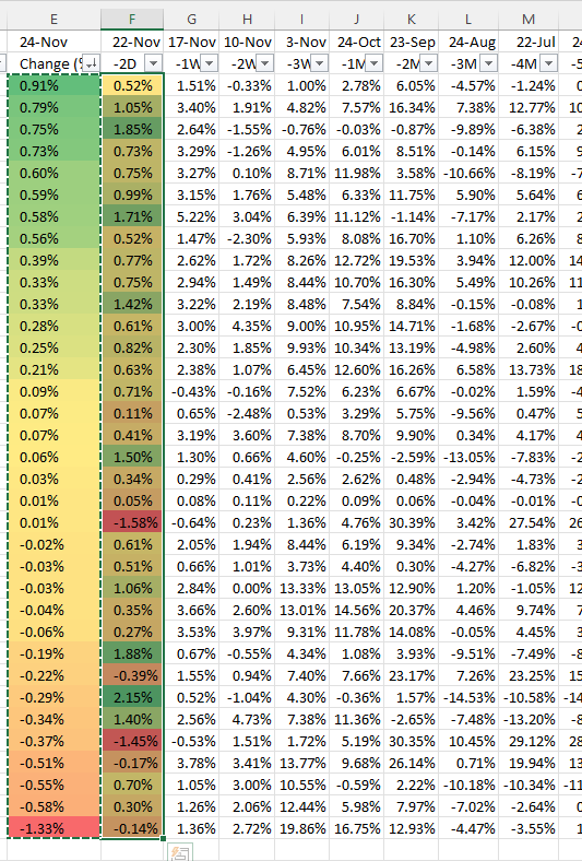
12. Repeat above steps with the remaining columns.
    

Back to top

Get Excel * .xlsx file

Back to top

 

Finance category

More than 1300 Excel formulas

Excel categories

Leave a Comment