How to use the TIME function
What is the TIME function?
The TIME function returns a decimal value between 0 (zero) representing 12:00:00 AM and 0.99988426 representing 11:59:59 P.M.
Formula in cell D3:
Table of Contents
- Syntax
- Arguments
- What is time in Excel?
- Example
- How to add hours
- How to add minutes
- How to add seconds
- How to calculate more than 24 hours?
- Convert time to 24 hour clock
- Function not working
- Get Excel *.xlsx file
- How to AVERAGE time
- How to sum overlapping time
- How to calculate overlapping time ranges
1. Syntax
TIME(hour, minute, second)
2. Arguments
| hour | Required. A number between 0 and 32767 represents the hour. |
| minute | Required. A number between 0 and 32767 represents the minute. |
| second | Required. A number between 0 and 32767 represents the second. |
3. What is time in Excel?

Excel time value is a number equal to or larger than 0 (zero) and smaller than 1, formatted as a time value. One hour is 1/24, there are 24 hours in one day.
One minute is 1/1440, there are 1440 minutes in one day (60*24 = 1440). One second is 1/86400, there are 86400 seconds in one day (60*60*24 = 86400).
The following table shows whole hours, one hour is 1/24, 2 hours is 2/24, and so on.
0 - 12:00:00 AM
1/24 - 1:00:00 AM
2/24 - 2:00:00 AM
...
23/24 - 11:00:00 PM
24/24 - 12:00:00 AM
The time value is only the decimal part of a number, in other words, a value larger than or equal to 1 makes no difference, Excel uses only the decimal part of a number to create an Excel time value.
1.5 -> 0.5 -> 12:00:00 PM
The whole numbers represent dates in Excel. The whole number and the decimal part create a date and time value. Here is an example: 1.5 represents 1/1/1900 12:00 PM
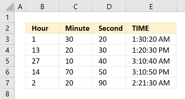
4. Example
The TIME function creates an Excel time value meaning a number equal to or larger than 0 (zero) and smaller than 1 formatted as a time value.
Formula in cell E3:
Explaining formula
Step 1 - TIME function
TIME(hour, minute, second)
Step 2 - Populate arguments
TIME(hour, minute, second)
hour - B3
minute - C3
second - D3
Step 3 - Evaluate formula
TIME(1, 30, 20)
and returns 0.062731481 (1:30:20 AM).
1 hour = 1/24
30 min = 30/1440
20 sec = 20/86400
1/24 + 30/1440 + 20/86400 = 0.062731481
4.1 Hour value larger than 24

An hour value greater than 23 will be divided by 24 and the remaining hours will be returned by the function.
27/24 = 1.125 The decimal part is 0.125 and is equal to 3 hours. 3/24 = 0.125
4.2 Minute value larger than 59

A minute value equal to or greater than 60 will be divided by 60, the whole number is hours and the remaining minutes will be minutes.
119/60 is approx. 1.983333 The TIME function returns 1:59:00 AM. 0.983333 is approx. 59 minutes.
4.3 Seconds value larger than 59

A "second" value equal to or greater than 60 will be divided by 60 and added to minutes, the remaining seconds are returned.
7200/86400 is approx. 0.083333 which is the same as 120 minutes or 2 hours.
5. How to add hours

Formula in cell F3:
Alternative formula:
Note, the TIME function arguments are limited to 32767. Larger values return #NUM errors.
Explaining formula
Step 1 - Calculate hours in decimals
D3/24
becomes
5/24 equals 0.208333333.
Step 2 - Add time
B3+D3/24
becomes
0.979166667 + 5/24
becomes
0.979166667 + 0.208333333 equals 1.1875
6. How to add minutes

Formula in cell F3:
Alternative formula:
Note, the TIME function arguments are limited to 32767. Larger values return #NUM errors.
Explaining formula
Step 1 - Calculate hours in decimals
The division slash charcater lets you divide numbers in an Excel formula.
D3/24
becomes
5/1440 is approx. 0.0034722
Step 2 - Add time
The plus sign lets you add numbers in an Excel formula.
B3+D3/1440
becomes
0.979166667 + 5/1440
becomes
0.979166667 + 0.0034722
and is approx. 0.982638889
7. How to add seconds

Formula in cell F3:
Alternative formula:
Note, the TIME function arguments are limited to 32767. Larger values return #NUM errors.
Explaining formula
Step 1 - Calculate seconds in decimals
D3/24
becomes
5/86400
and is approx. 0.0000578
Step 2 - Add time
B3+D3/24
becomes
0.979166667 + 5/86400
becomes
0.979166667 + 0.0000578
and is approx. 0.979224537037037
8. How to calculate more than 24 hours?

The image above shows how to display an Excel time value larger than 1. This is possible using a different cell formatting code than the default one Excel uses.
- Select cell F3.
- Press CTRL + 1 to open the "Format Cells" dialog box.
- Select the "Custom" category.
- Use the following formatting code:
[h]:mm:ss - Press with left mouse button on OK button.
Explaining formula in cell F3
Step 1 - Calculate Excel time value
Cell F3 contains an Excel time value larger than 1.
B3+B5/24
becomes
0.979166666666667 + B5/24
becomes
0.979166666666667 + 60/24
becomes
0.979166666666667 + 2.5
and returns 3.47916666666667 in cell F3. Cell F3 is formatted using the following cell formatting code: [h]:mm:ss which shows 83:30:00 in cell F3.
Step 2 - Verify calculation
We can easily verify the calculation.
3*24 = 72 hours
0.47916666666667 * 24 equals 11.5 hours.
72 + 11.5 = 83.5 hours -> 83:30:00
9. Convert time to 24 hour clock

The TEXT functionlets you convert AM/PM to a 24 hour clock.
Formula in cell D3:
Explaining formula
Step 1 - TEXT function
The TEXT function converts a value to text in a specific number format.
TEXT(value, format_text)
| value | The string you want to format. You can use a cell reference here or use a text string. |
| format_text | Formatting code allows you to change the way, for example, a date or a number is displayed to the Excel user. |
Step 2 - Populate TEXT function arguments
TEXT(value, format_text)
value - B3
format_text - "hh:mm:ss"
hh - hours using two digits
mm - minutes (two digits)
ss - seconds (two digits)
Step 3 - Evaluate TEXT function
TEXT(B3,"hh:mm:ss")
becomes
TEXT(0.0627314814814815, "hh:mm:ss")
and returns 01:30:20.
1/24 + 30/1440 + 20/86400 equals 0.0627314814814815.
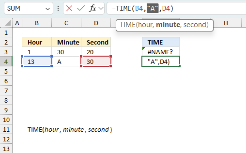
10. Function not working
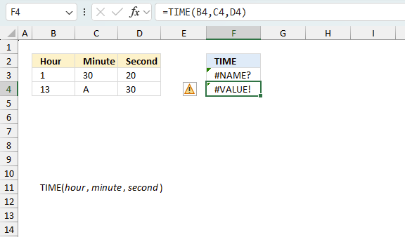
The TIME function returns
- #VALUE! error if you use a non-numeric input value.
- #NAME? error if you misspell the function name.
- propagates errors, meaning that if the input contains an error (e.g., #VALUE!, #REF!), the function will return the same error.
10.1 Troubleshooting the error value
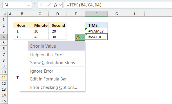
When you encounter an error value in a cell a warning symbol appears, displayed in the image above. Press with mouse on it to see a pop-up menu that lets you get more information about the error.
- The first line describes the error if you press with left mouse button on it.
- The second line opens a pane that explains the error in greater detail.
- The third line takes you to the "Evaluate Formula" tool, a dialog box appears allowing you to examine the formula in greater detail.
- This line lets you ignore the error value meaning the warning icon disappears, however, the error is still in the cell.
- The fifth line lets you edit the formula in the Formula bar.
- The sixth line opens the Excel settings so you can adjust the Error Checking Options.
Here are a few of the most common Excel errors you may encounter.
#NULL error - This error occurs most often if you by mistake use a space character in a formula where it shouldn't be. Excel interprets a space character as an intersection operator. If the ranges don't intersect an #NULL error is returned. The #NULL! error occurs when a formula attempts to calculate the intersection of two ranges that do not actually intersect. This can happen when the wrong range operator is used in the formula, or when the intersection operator (represented by a space character) is used between two ranges that do not overlap. To fix this error double check that the ranges referenced in the formula that use the intersection operator actually have cells in common.
#SPILL error - The #SPILL! error occurs only in version Excel 365 and is caused by a dynamic array being to large, meaning there are cells below and/or to the right that are not empty. This prevents the dynamic array formula expanding into new empty cells.
#DIV/0 error - This error happens if you try to divide a number by 0 (zero) or a value that equates to zero which is not possible mathematically.
#VALUE error - The #VALUE error occurs when a formula has a value that is of the wrong data type. Such as text where a number is expected or when dates are evaluated as text.
#REF error - The #REF error happens when a cell reference is invalid. This can happen if a cell is deleted that is referenced by a formula.
#NAME error - The #NAME error happens if you misspelled a function or a named range.
#NUM error - The #NUM error shows up when you try to use invalid numeric values in formulas, like square root of a negative number.
#N/A error - The #N/A error happens when a value is not available for a formula or found in a given cell range, for example in the VLOOKUP or MATCH functions.
#GETTING_DATA error - The #GETTING_DATA error shows while external sources are loading, this can indicate a delay in fetching the data or that the external source is unavailable right now.
10.2 The formula returns an unexpected value
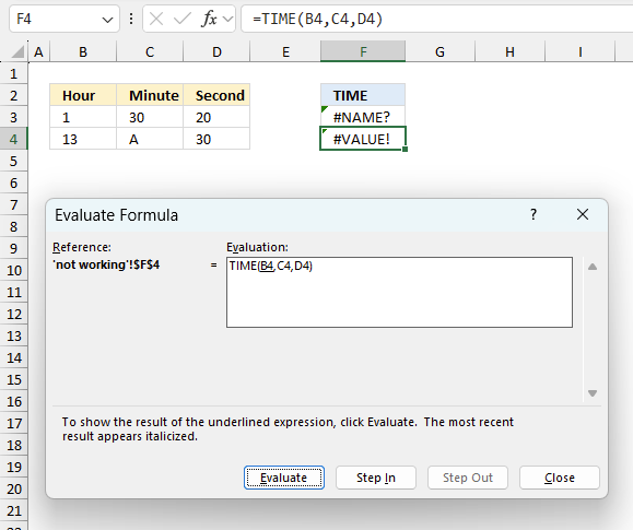
To understand why a formula returns an unexpected value we need to examine the calculations steps in detail. Luckily, Excel has a tool that is really handy in these situations. Here is how to troubleshoot a formula:
- Select the cell containing the formula you want to examine in detail.
- Go to tab “Formulas” on the ribbon.
- Press with left mouse button on "Evaluate Formula" button. A dialog box appears.
The formula appears in a white field inside the dialog box. Underlined expressions are calculations being processed in the next step. The italicized expression is the most recent result. The buttons at the bottom of the dialog box allows you to evaluate the formula in smaller calculations which you control. - Press with left mouse button on the "Evaluate" button located at the bottom of the dialog box to process the underlined expression.
- Repeat pressing the "Evaluate" button until you have seen all calculations step by step. This allows you to examine the formula in greater detail and hopefully find the culprit.
- Press "Close" button to dismiss the dialog box.
There is also another way to debug formulas using the function key F9. F9 is especially useful if you have a feeling that a specific part of the formula is the issue, this makes it faster than the "Evaluate Formula" tool since you don't need to go through all calculations to find the issue.
- Enter Edit mode: Double-press with left mouse button on the cell or press F2 to enter Edit mode for the formula.
- Select part of the formula: Highlight the specific part of the formula you want to evaluate. You can select and evaluate any part of the formula that could work as a standalone formula.
- Press F9: This will calculate and display the result of just that selected portion.
- Evaluate step-by-step: You can select and evaluate different parts of the formula to see intermediate results.
- Check for errors: This allows you to pinpoint which part of a complex formula may be causing an error.
The image above shows cell reference C3 converted to hard-coded value using the F9 key. The TIME function requires numerical values which is not the case in this example. We have found what is wrong with the formula.
Tips!
- View actual values: Selecting a cell reference and pressing F9 will show the actual values in those cells.
- Exit safely: Press Esc to exit Edit mode without changing the formula. Don't press Enter, as that would replace the formula part with the calculated value.
- Full recalculation: Pressing F9 outside of Edit mode will recalculate all formulas in the workbook.
Remember to be careful not to accidentally overwrite parts of your formula when using F9. Always exit with Esc rather than Enter to preserve the original formula. However, if you make a mistake overwriting the formula it is not the end of the world. You can “undo” the action by pressing keyboard shortcut keys CTRL + z or pressing the “Undo” button
10.3 Other errors
Floating-point arithmetic may give inaccurate results in Excel - Article
Floating-point errors are usually very small, often beyond the 15th decimal place, and in most cases don't affect calculations significantly.
11. How to AVERAGE time
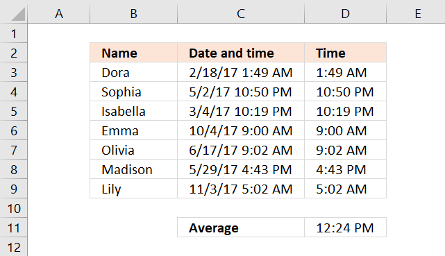
Table of Contents
- How to AVERAGE time
- How to enter an array formula
- Explaining formula
- How to calculate the average of multiple time differences in this format: hours, minutes, and seconds
- Get Excel *.xlsx file
11.1. How to AVERAGE time
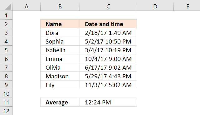
The image above shows names in cells B3 to B9 and corresponding date and time values in cells C3 to C9.
The formula demonstrated in cell C11 calculates the average time of day across the dates and times listed in cells C3 through C9. However, it doesn't take the date part into the calculations which would skew the average and return an incorrect value.
This formula effectively ignores the date part and focuses only on the time of day. The result is the average time, which in this case is shown as 12:24 PM in cell C11.
This approach is useful when you want to find the average time regardless of the dates on which those times occurred.
Here's how it basically works:
- C3:C9 refers to the range of cells containing the date and time values.
- INT(C3:C9) extracts just the integer part of each date/time value, which represents the date portion.
- C3:C9 - INT(C3:C9) subtracts the date portion from the original date/time value, leaving only the time portion. In Excel, times are stored as fractional parts of a day.
- AVERAGE() then calculates the mean of these time values.
11.1.1 How to enter an array formula
You need to enter the formula as an array formula if you use an earlier version than Excel 365.
The formula above is an array formula. To enter an array formula, type the formula in a cell then press and hold CTRL + SHIFT simultaneously, now press Enter once. Release all keys.

The formula bar now shows the formula enclosed with curly brackets telling you that you entered the formula successfully. Don't enter the curly brackets yourself.
11.1.2 Explaining formula
An Excel date and time value is in fact a number and a decimal part formatted as a date. For example, number 1 is 1/1/1900 and 1.5 is 1/1/1900 12:00 PM. This makes it really easy to add or subtract days to dates in Excel.
Step 1 - Extract whole numbers
The INT function returns the integer part of a number.
INT(number)
INT(C3:C9)
returns {42784; 42857; ... ; 43042}.
Notice how the values lost their decimal part, only the whole numbers remains.
Step 2 - Extract decimals
The date part is the whole number and the decimals are the times, we can extract the time part by subtracting the original numbers with the whole numbers.
The minus sign lets you subtract a number with another number in Excel formulas.
C3:C9 -INT(C3:C9)
returns {0.0758894520549802; ... ; 0.209842259464494}
Step 3 - Average decmial numbers
The AVERAGE function calculates an average.
AVERAGE(number1, [number2], ...)
AVERAGE(C3:C9 -INT(C3:C9))
becomes
AVERAGE({0.0758894520549802; ... ; 0.209842259464494})
and returns 0.516732388989892.
11.2. How to calculate the average of multiple time differences in this format: hours, minutes, and seconds

This example demonstrates a formula and cell formatting that allows you to calculate the mean of differences between date and time values across two columns. The cell formatting lets you show hours larger than the regular 24 hours per day meaning it shows the accumulated value in hours, minutes, and seconds.
The image shows an Excel spreadsheet with two columns of date and time data, and a calculation of the average difference between these times. Column B contains a set of dates and times, ranging from 2/18/17 1:49 AM to 11/3/17 5:02 AM. Column C contains another set of dates and times, ranging from 5/4/17 2:53 PM to 1/1/18 12:10 AM.
| Date and time | Date and time |
| 2/18/17 1:49 AM | 5/4/17 2:53 PM |
| 5/2/17 10:50 PM | 6/13/17 10:40 PM |
| 3/4/17 10:19 PM | 4/4/17 10:27 PM |
| 10/4/17 9:00 AM | 12/7/17 4:49 PM |
| 6/17/17 9:02 AM | 7/3/17 12:07 PM |
| 5/29/17 4:43 PM | 7/9/17 2:57 PM |
| 11/3/17 5:02 AM | 1/1/18 12:10 AM |
The formula in cell C11 calculates an average based on the differences of the Excel dates and time values in columns C and B.
Formula in cell C11:
The result shown in cell C11 is 1127:02:50, which represents 1127 hours, 2 minutes, and 50 seconds. This is equivalent to about 47 days.
This calculation gives the average time span between the dates in column B and the dates in column C. It's important to note that this method assumes that all dates in column C are later than their corresponding dates in column B. If any dates in column C are earlier, it would lead to unexpected results.
The cell C11 formatting allows to display the average time in accumulated hours, minute, and seconds instead of days, hours, minute, and seconds.
Cell formatting is applied to cell C11:
- Select cell C11.
- Press CTRL + 1 to open the "Format Cells" dialog box, see the image above.
- Press with left mouse button on "Custom" category.
- Enter a new "type": [hh]:mm:ss
- Press with left mouse button on OK button.
The difference between the two cell formats in Excel is:
- 1. [hh]:mm:ss This format treats the hours as a number in square brackets, rather than a standard time format. The hours value can be greater than 24, as it represents the total number of hours, not just the hour of the day. This format is useful for displaying long durations larger than 24 hours.
- hh:mm:ss The hours value is limited to 0-23, representing the hour of the day. This format is better suited for displaying times within a 24-hour period.
If the value is 25:30:15, in the [hh]:mm:ss format it would display as 25:30:15 indicating a duration of 25 hours, 30 minutes, and 15 seconds. In the hh:mm:ss format, the same value would display as 01:30:15, which represents 1 hour, 30 minutes, and 15 seconds, however 24 hours are missing. The choice of format depends on whether you need to display durations that is longer than 24 hours or if you're working with times within a single day.
11.2.1 Explaining formula
An Excel date and time value is in fact a number and a decimal part formatted as a date. For example, number 1 is 1/1/1900 and 1.5 is 1/1/1900 12:00 PM. This makes it really easy to add or subtract dates in Excel.
Step 1 - Calculate difference between date and time values
The minus sign lets you subtract a number with another number in Excel formulas.
C3:C9-B3:B9
returns {75.5446924890348; ... ; 58.7977072514477}.
Step 2 - Calculate the average
The AVERAGE function calculates an average.
AVERAGE(number1, [number2], ...)
AVERAGE(C3:C9-B3:B9)
becomes
AVERAGE({75.5446924890348; ... ; 58.7977072514477})
and returns approx. 46.96 in cell C11, however, the value is formatted to show total hours, seconds and milliseconds.
11.3 Get Excel *.xlsx file
12. How to sum overlapping time
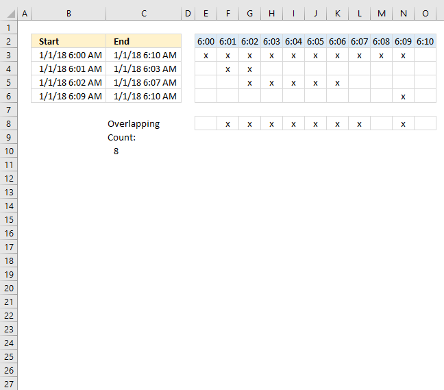
The worksheet above shows four different time ranges in column B and C, the formula in cell C10 counts the number of overlapping minutes.
The formula uses the earliest and latest date and time value in column B and C as the range to count overlapping minutes.
What's on this section
- Sum overlapping time
- Sum overlapping time based on a date range
- Sum overlapping time - Excel 365
12.1. Sum overlapping time
Array formula in cell C10:
To enter an array formula, type the formula in a cell then press and hold CTRL + SHIFT simultaneously, now press Enter once. Release all keys.
The formula bar now shows the formula with a beginning and ending curly bracket telling you that you entered the formula successfully. Don't enter the curly brackets yourself.
12.1.2 Explaining formula in cell C10
The INDEX function allows you to create an array of values, in this case, minute intervals.
MIN($B$3:$B$6)+(ROW(A1:INDEX($A:$A, (MAX($C$3:$C$6)-MIN($B$3:$B$6))*1440+1))-1)/1440
returns
{43101.25, 43101.2506944444, 43101.2513888889, 43101.2520833333, 43101.2527777778, 43101.2534722222, 43101.2541666667, 43101.2548611111, 43101.2555555556, 43101.25625, 43101.2569444444}
Now check if these minute intervals are between or equal to each date and time range.
(TRANSPOSE(MIN($B$3:$B$6)+(ROW(A1:INDEX($A:$A, (MAX($C$3:$C$6)-MIN($B$3:$B$6))*1440+1))-1)/1440)>=$B$3:$B$6)*((TRANSPOSE(MIN($B$3:$B$6)+(ROW(A1:INDEX($A:$A, (MAX($C$3:$C$6)-MIN($B$3:$B$6))*1440+1))-1)/1440))<$C$3:$C$6)
returns
{1, 1, 1, 1, 1, 1, 1, 1, 1, 1, 0; 0, 1, 1, 1, 0, 0, 0, 0, 0, 0, 0; 0, 0, 1, 1, 1, 1, 1, 1, 0, 0, 0; 0, 0, 0, 0, 0, 0, 0, 0, 0, 1, 0}
The MMULT function allows you to add these values column by column.
MMULT(TRANSPOSE($B$3:$B$6^0), (TRANSPOSE(MIN($B$3:$B$6)+(ROW(A1:INDEX($A:$A, (MAX($C$3:$C$6)-MIN($B$3:$B$6))*1440+1))-1)/1440)>=$B$3:$B$6)*((TRANSPOSE(MIN($B$3:$B$6)+(ROW(A1:INDEX($A:$A, (MAX($C$3:$C$6)-MIN($B$3:$B$6))*1440+1))-1)/1440))<$C$3:$C$6))
becomes
MMULT(TRANSPOSE($B$3:$B$6^0), {1, 1, 1, 1, 1, 1, 1, 1, 1, 1, 0; 0, 1, 1, 1, 0, 0, 0, 0, 0, 0, 0; 0, 0, 1, 1, 1, 1, 1, 1, 0, 0, 0; 0, 0, 0, 0, 0, 0, 0, 0, 0, 1, 0})
becomes
MMULT({1,1,1,1}, {1, 1, 1, 1, 1, 1, 1, 1, 1, 1, 0; 0, 1, 1, 1, 0, 0, 0, 0, 0, 0, 0; 0, 0, 1, 1, 1, 1, 1, 1, 0, 0, 0; 0, 0, 0, 0, 0, 0, 0, 0, 0, 1, 0})
and returns
{1, 2, 3, 3, 2, 2, 2, 2, 1, 2, 0}
The following picture shows the array and what the MMULT function returns.
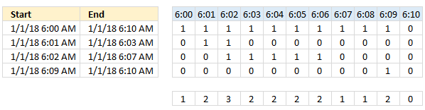
A value larger than 1 indicates an overlapping time value.
MMULT(TRANSPOSE($B$3:$B$6^0), (TRANSPOSE(MIN($B$3:$B$6)+(ROW(A1:INDEX($A:$A, (MAX($C$3:$C$6)-MIN($B$3:$B$6))*1440+1))-1)/1440)>=$B$3:$B$6)*((TRANSPOSE(MIN($B$3:$B$6)+(ROW(A1:INDEX($A:$A, (MAX($C$3:$C$6)-MIN($B$3:$B$6))*1440+1))-1)/1440))<=$C$3:$C$6))>1
becomes
{1, 2, 3, 3, 2, 2, 2, 2, 1, 2, 0}>1
and returns
{FALSE, TRUE, TRUE, TRUE, TRUE, TRUE, TRUE, TRUE, FALSE, TRUE, FALSE}.
Lastly, multiply with 1 to convert boolean values to numerical values and then sum the numbers.
SUM((MMULT(TRANSPOSE($B$3:$B$6^0), (TRANSPOSE(MIN($B$3:$B$6)+(ROW(A1:INDEX($A:$A, (MAX($C$3:$C$6)-MIN($B$3:$B$6))*1440+1))-1)/1440)>=$B$3:$B$6)*((TRANSPOSE(MIN($B$3:$B$6)+(ROW(A1:INDEX($A:$A, (MAX($C$3:$C$6)-MIN($B$3:$B$6))*1440+1))-1)/1440))<=$C$3:$C$6))>1)*1)
becomes
SUM({FALSE, TRUE, TRUE, TRUE, TRUE, TRUE, TRUE, TRUE, FALSE, TRUE, FALSE}*1)
becomes
SUM({0,1,1,1,1,1,1,1,0,1,0})
and returns 8.
12.2 Sum overlapping time based on a date range
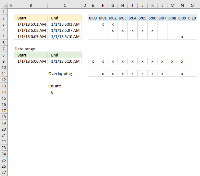
The picture above shows you a different setup, it allows you to use a smaller range than the min and max date and time in B3:C5.
Formula in cell C14:
The ROW function limits the use of these formulas, if you have a range larger than 1,048,576 minutes, which is the same as the number of rows in a worksheet, you will need another solution than the one presented here.
Get Excel *.xlsx file
How to count overlapping timev3.xlsx
12.3. Sum overlapping time - Excel 365
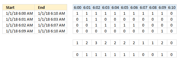
This Excel 365 formula works just like the formula in section 1.1 above, however, the SEQUENCE and LET functions simplify and shorten the formula considerably.
Dynamic array formula in cell C10:
Explaining formula
The date and time values are actually numbers, dates are whole numbers. 1 is 1/1/1900 and the next day 1/2/1900 is 2 and so on. Decimal numbers are time values in Excel, for example:
00:00 AM is 0 (zero)
12:00 PM is 0.5
The whole number and the decimal number together form a date and time value in Excel. 1.5 is 1/1/1900 12:00 PM.
Step 1 - Subtract numbers
The minus sign lets you subtract numbers in Excel formulas, this example calculates a number representing the difference between the two date and time values specified in cells C9 and B9.
C9-B9
becomes
43101.2569444445 - 43101.25
and returns 0.00694444450346055
Step 2 - Multiply with 1440
The asterisk lets you multiply numbers in an Excel formula. There are 60 minutes in one hour, and twenty-four hours in one day. 60*24 equals 1440.
(C9-B9)*1440
becomes
0.00694444450346055*1440
and returns
10.0000000849832
Step 3 - Add 1
The plus sign lets you add numbers in an Excel formula.
(C9-B9)*1440+1
becomes
10.0000000849832+1
and returns
11.0000000849832
Step 4 - Create a sequence of numbers
The SEQUENCE function creates a list of sequential numbers.
Function syntax: SEQUENCE(rows, [columns], [start], [step])
SEQUENCE(,(C9-B9)*1440+1,0)
becomes
SEQUENCE(,11.0000000849832,0)
and returns
{0, 1, 2, 3, 4, 5, 6, 7, 8, 9, 10}.
SEQUENCE(,(C9-B9)*1440+1,0)/1440
becomes
{0, 1, 2, 3, 4, 5, 6, 7, 8, 9, 10}/1440
and returns
{0, 0.000694444444444444, 0.00138888888888889, 0.00208333333333333, 0.00277777777777778, 0.00347222222222222, 0.00416666666666667, 0.00486111111111111, 0.00555555555555556, 0.00625, 0.00694444444444444}
Step 5 - Add sequence to start date
B9+SEQUENCE(,(C9-B9)*1440+1,0)/1440
becomes
43101.25 + {0, 0.000694444444444444, 0.00138888888888889, 0.00208333333333333, 0.00277777777777778, 0.00347222222222222, 0.00416666666666667, 0.00486111111111111, 0.00555555555555556, 0.00625, 0.00694444444444444}
and returns
{43101.25, 43101.2506944444, 43101.2513888889, 43101.2520833333, 43101.2527777778, 43101.2534722222, 43101.2541666667, 43101.2548611111, 43101.2555555556, 43101.25625, 43101.2569444444}
Step 6 - Check if values in array is larger or equal to each value in cell range B3:B5
The larger than sign and the equal signs are logical operators, they return TRUE or FALSE if a condition is met or not.
(B9+SEQUENCE(,(C9-B9)*1440+1,0)/1440)>=B3:B5
becomes
{43101.25, 43101.2506944444, 43101.2513888889, 43101.2520833333, 43101.2527777778, 43101.2534722222, 43101.2541666667, 43101.2548611111, 43101.2555555556, 43101.25625, 43101.2569444444}>={43101.2506944444; 43101.2513888889; 43101.25625}
and returns
{FALSE, TRUE, TRUE, TRUE, TRUE, TRUE, TRUE, TRUE, TRUE, TRUE, TRUE;FALSE, FALSE, TRUE, TRUE, TRUE, TRUE, TRUE, TRUE, TRUE, TRUE, TRUE;FALSE, FALSE, FALSE, FALSE, FALSE, FALSE, FALSE, FALSE, FALSE, TRUE, TRUE}
Step 7 - Check if values in array is smaller to each value in cell range B3:B5
(B9+SEQUENCE(,(C9-B9)*1440+1,0)/1440)<C3:C5
becomes
{43101.25, 43101.2506944444, 43101.2513888889, 43101.2520833333, 43101.2527777778, 43101.2534722222, 43101.2541666667, 43101.2548611111, 43101.2555555556, 43101.25625, 43101.2569444444}<{43101.2520833333; 43101.2548611111; 43101.2569444445}
and returns
{TRUE, TRUE, TRUE, FALSE, FALSE, FALSE, FALSE, FALSE, FALSE, FALSE, FALSE;TRUE, TRUE, TRUE, TRUE, TRUE, TRUE, TRUE, FALSE, FALSE, FALSE, FALSE;TRUE, TRUE, TRUE, TRUE, TRUE, TRUE, TRUE, TRUE, TRUE, TRUE, TRUE}
Step 8 - Multiply arrays (AND logic)
The asterisk character lets you multiply numbers in an Excel formula, the equivalent function would be the PRODUCT function.
((B9+SEQUENCE(,(C9-B9)*1440+1,0)/1440)>=B3:B5)*((B9+SEQUENCE(,(C9-B9)*1440+1,0)/1440)<C3:C5)
becomes
{FALSE, TRUE, TRUE, TRUE, TRUE, TRUE, TRUE, TRUE, TRUE, TRUE, TRUE;FALSE, FALSE, TRUE, TRUE, TRUE, TRUE, TRUE, TRUE, TRUE, TRUE, TRUE;FALSE, FALSE, FALSE, FALSE, FALSE, FALSE, FALSE, FALSE, FALSE, TRUE, TRUE}*{TRUE, TRUE, TRUE, FALSE, FALSE, FALSE, FALSE, FALSE, FALSE, FALSE, FALSE;TRUE, TRUE, TRUE, TRUE, TRUE, TRUE, TRUE, FALSE, FALSE, FALSE, FALSE;TRUE, TRUE, TRUE, TRUE, TRUE, TRUE, TRUE, TRUE, TRUE, TRUE, TRUE}
and returns
{0, 1, 1, 0, 0, 0, 0, 0, 0, 0, 0;0, 0, 1, 1, 1, 1, 1, 0, 0, 0, 0;0, 0, 0, 0, 0, 0, 0, 0, 0, 1, 1}.
When you multiply boolean values TRUE or FALSE the result is their numerical equivalent:
TRUE = 1
FALSE = 0 (zero)
Step 9 - Check if result is larger than 0 (zero)
((B9+SEQUENCE(,(C9-B9)*1440+1,0)/1440)>=B3:B5)*((B9+SEQUENCE(,(C9-B9)*1440+1,0)/1440)<C3:C5)>0
becomes
{0, 1, 1, 0, 0, 0, 0, 0, 0, 0, 0;0, 0, 1, 1, 1, 1, 1, 0, 0, 0, 0;0, 0, 0, 0, 0, 0, 0, 0, 0, 1, 1}>0
and returns
{FALSE, TRUE, TRUE, FALSE, FALSE, FALSE, FALSE, FALSE, FALSE, FALSE, FALSE;FALSE, FALSE, TRUE, TRUE, TRUE, TRUE, TRUE, FALSE, FALSE, FALSE, FALSE;FALSE, FALSE, FALSE, FALSE, FALSE, FALSE, FALSE, FALSE, FALSE, TRUE, TRUE}.
Step 10 - Rearrange vertical values to horizontal values
The TRANSPOSE function converts a vertical range to a horizontal range, or vice versa.
Function syntax: TRANSPOSE(array)
TRANSPOSE(B3:B5^0)
becomes
TRANSPOSE({43101.2506944444; 43101.2513888889; 43101.25625}^0)
becomes
TRANSPOSE({1; 1; 1})
and returns
{1, 1, 1}.
Step 11 - Convert boolean values to their numerical equivalents
(((B9+SEQUENCE(,(C9-B9)*1440+1,0)/1440)>=B3:B5)*((B9+SEQUENCE(,(C9-B9)*1440+1,0)/1440)<C3:C5)>0)*1
becomes
{FALSE, TRUE, TRUE, FALSE, FALSE, FALSE, FALSE, FALSE, FALSE, FALSE, FALSE;FALSE, FALSE, TRUE, TRUE, TRUE, TRUE, TRUE, FALSE, FALSE, FALSE, FALSE;FALSE, FALSE, FALSE, FALSE, FALSE, FALSE, FALSE, FALSE, FALSE, TRUE, TRUE}*1
and returns
{0, 1, 1, 0, 0, 0, 0, 0, 0, 0, 0;0, 0, 1, 1, 1, 1, 1, 0, 0, 0, 0;0, 0, 0, 0, 0, 0, 0, 0, 0, 1, 1}
Step 12 - Calculate the matrix product of two arrays
The MMULT function calculates the matrix product of two arrays, an array as the same number of rows as array1 and columns as array2.
Function syntax: MMULT(array1, array2)
MMULT(TRANSPOSE(B3:B5^0),(((B9+SEQUENCE(,(C9-B9)*1440+1,0)/1440)>=B3:B5)*((B9+SEQUENCE(,(C9-B9)*1440+1,0)/1440)<C3:C5)>0)*1)
becomes
MMULT({1, 1, 1},{0, 1, 1, 0, 0, 0, 0, 0, 0, 0, 0;0, 0, 1, 1, 1, 1, 1, 0, 0, 0, 0;0, 0, 0, 0, 0, 0, 0, 0, 0, 1, 1})
and returns
{0, 1, 2, 1, 1, 1, 1, 0, 0, 1, 1}
Step 13 - Check if result is larger than 0 (zero)
MMULT(TRANSPOSE(B3:B5^0),(((B9+SEQUENCE(,(C9-B9)*1440+1,0)/1440)>=B3:B5)*((B9+SEQUENCE(,(C9-B9)*1440+1,0)/1440)<C3:C5)>0)*1)>0
becomes
{0, 1, 2, 1, 1, 1, 1, 0, 0, 1, 1}>0
and returns
{FALSE, TRUE, TRUE, TRUE, TRUE, TRUE, TRUE, FALSE, FALSE, TRUE, TRUE}.
Step 14 - Convert boolean values to numerical equivalents
(MMULT(TRANSPOSE(B3:B5^0),(((B9+SEQUENCE(,(C9-B9)*1440+1,0)/1440)>=B3:B5)*((B9+SEQUENCE(,(C9-B9)*1440+1,0)/1440)<C3:C5)>0)*1)>0)*1
becomes
{FALSE, TRUE, TRUE, TRUE, TRUE, TRUE, TRUE, FALSE, FALSE, TRUE, TRUE}*1
and returns
{0, 1, 1, 1, 1, 1, 1, 0, 0, 1, 1}.
Step 15 - Add numbers in array and return a total
The SUM function allows you to add numerical values, the function returns the sum in the cell it is entered in. The SUM function is cleverly designed to ignore text and boolean values, adding only numbers.
Function syntax: SUM(number1, [number2], ...)
SUM((MMULT(TRANSPOSE(B3:B5^0),(((B9+SEQUENCE(,(C9-B9)*1440+1,0)/1440)>=B3:B5)*((B9+SEQUENCE(,(C9-B9)*1440+1,0)/1440)<C3:C5)>0)*1)>0)*1)
becomes
SUM({0, 1, 1, 1, 1, 1, 1, 0, 0, 1, 1})
and returns 8.
Step 16 - Shorten formula
The LET function lets you name intermediate calculation results which can shorten formulas considerably and improve performance.
Function syntax: LET(name1, name_value1, calculation_or_name2, [name_value2, calculation_or_name3...])
SUM((MMULT(TRANSPOSE(B3:B5^0),(((B9+SEQUENCE(,(C9-B9)*1440+1,0)/1440)>=B3:B5)*((B9+SEQUENCE(,(C9-B9)*1440+1,0)/1440)<C3:C5)>0)*1)>0)*1)
y - B3:B5
x - B9+SEQUENCE(,(C9-B9)*1440+1,0)/1440
LET(y,B3:B5,x,B9+SEQUENCE(,(C9-B9)*1440+1,0)/1440,SUM((MMULT(TRANSPOSE(y^0),(((x)>=y)*((x)<C3:C5)>0)*1)>0)*1))
13. How to calculate overlapping time ranges

I found an old post that I think is interesting to write about today. Think of two overlapping ranges, it may be dates, times, or any numerical range, the formula demonstrated here works with everything.
This picture shows two time ranges, 06:00-13:00 (yellow) and 11:00-18:00 (green).
It is obvious that there are two overlapping hours but how do we calculate how much they overlap in Excel?
The MEDIAN function comes to the rescue, but first, let me explain the function. It returns a value that separates the higher half of a data set from the lower half. Example, MEDIAN(1,2,3) returns 2. 1 is the lower half and 3 is the higher half.
MEDIAN(1,2,3,4,5,6) returns 3.5 because there are two values (3, 4) separating the higher half (5,6) from the lower half (1,2). The average of these two values is 3.5.
What's on this section
- Calculate overlapping hours
- Calculate total cost based on different rates per hour
- Calculate total cost based on different rates per hour (smaller formula)
- Calculate total cost based on different rates per hour across days
- Get Excel file
13.1. Calculate overlapping hours
We have 4 times here to remember, the start and end of time range 1 and 2.
Let see what happens if we use the MEDIAN function with the start and end value of time range 1 and only the start value of time range 2.
MEDIAN("6:00 AM", "01:00 PM", "11:00 AM") returns 11:00 AM.
And then the end of time range 2.
MEDIAN("6:00 AM", "01:00 PM", "06:00 PM") returns 01:00 PM
01:00 PM - 11:00 AM is 02:00. Two hours are overlapping.
The formula becomes
and returns 02:00.
13.2. Calculate total cost based on different rates per hour

The rate is 8 between 12:00 AM and 08:00 AM, 08:00 AM - 6:00 PM the rate is 5 and 6:00 PM to 12:00 AM the rate is 10.
How do we calculate total cost if the time range is 06:00 AM - 8:00 PM?
Count overlapping hours for the first range 00:00-08:00 and multiply with rate 8.
returns 16.
Count overlapping hours for the second range 08:00-18:00 and multiply with rate 5.
returns 50
Count overlapping hours for the second range 18:00-24:00 and multiply with rate 10.
returns 20.
Combining all formulas gives
returns 86.
13.2.1 I have a question for you
It would be great to build an array formula to shrink the formula above, like this one:
But it won't work, you can't use the MEDIAN function to do that. Do you know a workaround? See next section.
13.3. Calculate total cost based on different rates per hour (smaller formula)

The image above demonstrates a formula that calculates the total cost based on rates per hour. Check out Alex Grobermans formula in the comments section below.
The formula above won't work if you start and end spans over multiple days, see next section below.
Explaining calculation in cell C10
Step 1 - Calculate hour
The HOUR function returns an integer representing the hour of an Excel time value.
HOUR(C7)
becomes
HOUR(42005.25)
and returns 6.
Step 2 - Create cell reference
The INDIRECT function creates a cell reference based on text values.
INDIRECT("A"&HOUR(C7)+1&":A"&HOUR(C8))
becomes
INDIRECT("A"&6+1&":A"&12)
becomes
INDIRECT("A"&7&":A"&12)
becomes
INDIRECT("A7:A12")
and returns A7:A12.
Step 3 - Create row numbers
The ROW function returns row numbers from a cell reference.
ROW(INDIRECT("A"&HOUR(C7)+1&":A"&HOUR(C8)))
becomes
ROW(A7:A12)
and returns {7; 8; 9; 10; 11; 12}.
Step 4 - Calculate frequency based on time intervals
The FREQUENCY function calculates how often values occur within a range of values and returns a vertical array of numbers. It returns an array that is one more item larger than the bins_array.
FREQUENCY(data_array, bins_array)
FREQUENCY(ROW(INDIRECT("A"&HOUR(C7)+1&":A"&HOUR(C8))), HOUR(D3:D4))
becomes
FREQUENCY({7; 8; 9; 10; 11; 12}, {8;18})
and returns {2; 4; 0}.
Step 5 - Multiply with rates and return a total
The SUMPRODUCT function calculates the product of corresponding values and then returns the sum of each multiplication.
SUMPRODUCT(array1, [array2], ...)
SUMPRODUCT(FREQUENCY(ROW(INDIRECT("A"&HOUR(C7)+1&":A"&HOUR(C8))), HOUR(D3:D4)), E3:E5)
becomes
SUMPRODUCT({2; 4; 0}, E3:E5)
becomes
SUMPRODUCT({2; 4; 0}, {8;5;10})
and returns 36.
13.4. Calculate total cost based on different rates per hour across days

Alex Groberman contributed with an interesting formula, check out that comment below. I modified that formula and came up with this in order to get it working with a range that spans over multiple days.
Array formula in cell C10:
The formula above works with all Excel versions, the formula below is smaller, however, it works only in Excel 365:
Explaining calculation in cell C10

Press with left mouse button on the image above to see a larger version. The image shows the time range from start (cell C7) 1/1/2015 6:00 AM to end (cell C8) 1/1/2015 12:00 PM.
'TIME' function examples
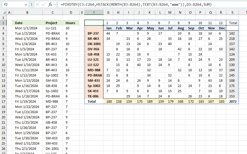
Tracking work hours across multiple projects can be challenging but Excel makes it easy with built-in functions. In this guide, […]
Functions in 'Date and Time' category
The TIME function function is one of 22 functions in the 'Date and Time' category.
Excel function categories
Excel categories
3 Responses to “How to use the TIME function”
Leave a Reply
How to comment
How to add a formula to your comment
<code>Insert your formula here.</code>
Convert less than and larger than signs
Use html character entities instead of less than and larger than signs.
< becomes < and > becomes >
How to add VBA code to your comment
[vb 1="vbnet" language=","]
Put your VBA code here.
[/vb]
How to add a picture to your comment:
Upload picture to postimage.org or imgur
Paste image link to your comment.
how to less three small time from average time
like
08:30
07:36
06:40
05:30
08:30
09:40
rahul kushwah,
can you explain in greater detail?
Thank you.