How to extract numbers from a cell value
Working with numbers in Excel can be deceptively tricky, especially when they're embedded within text or need to be formatted just right. Whether you're cleaning up messy data, extracting digits for analysis, or just trying to make your spreadsheets look more polished, knowing how to handle numbers in various scenarios can save you tons of time.
In this guide, we’ll walk you through practical techniques for extracting, sorting, and formatting numbers in Excel. From pulling out single digits to removing all numbers entirely, and from handling data in Excel 2016 to taking advantage of new functions in Excel 365, we’ve got you covered. Let’s dive in and make working with numbers a breeze.
What's on this page
- Introduction
- How to extract numbers from a cell value - Excel 2019
- Sort and return unique distinct single digits from cell range - Excel 365
- Extract numbers from a column
- Extract numbers from a column - Excel 365
- Extract numbers from a column - earlier Excel versions
- How to remove numbers from a cell value (Excel 2016)
- How to remove numbers from a cell value (Excel 365)
- How to format numbers as text
1. Introduction
When was the TEXTJOIN function introduced in Excel?
The TEXTJOIN function is available for Excel 2019 and later Excel versions.
Why remove numbers?
Clean up text data - Example: Turning "Product123" into "Product" when only the name is needed. Standardize formatting - For example, removing digits from "Room 402B" to make it just "Room B" for a standardized list. Prepare for comparison or lookup - You might need to match "Item12" and "Item" — removing numbers helps normalize the data.
Hide sensitive numeric data - Like removing part of an ID or a price embedded in text, e.g., "PlanA_299" → "PlanA". For presentation/reporting - You may want to show cleaner labels like "Customer45" → "Customer". Extract only alphabetic tags - Useful if you’re parsing a mixed input like "Dept42XYZ", and you only care about "DeptXYZ".
Why extract numbers from a cell value?
Use numbers for calculation - Example: Extracting "45" from "Order #45" so you can sort, analyze, or sum orders. Split metadata - Like pulling "123" from "Invoice123" to store in a separate column for invoice tracking. Normalize data formats - For example, turning "ID: AB-10923" into "10923" for importing into another system.
Filter or group by numeric values - Extracting digits helps you group entries like "Batch20A", "Batch20B", etc., by the number. Generate IDs or keys - You might extract numbers to create unique identifiers or reference codes. Validate or check patterns - Pulling the numbers out of "AB1234" helps check if the number falls within a valid range.
2. How to extract numbers from a cell value - Excel 2019
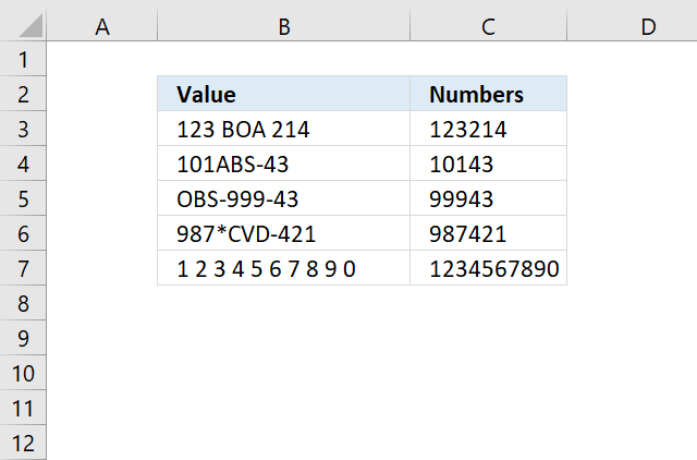
The following array formula, demonstrated in cell C3, extracts all numbers from a cell value:
To enter an array formula, type the formula in a cell then press and hold CTRL + SHIFT simultaneously, now press Enter once. Release all keys.
The formula bar now shows the formula with a beginning and ending curly bracket telling you that you entered the formula successfully. Don't enter the curly brackets yourself.
If your cell contains more than a 1000 characters change this part of the formula $A$1:$A$1000 to perhaps $A$1:$A$2000 depending on how many characters you have.
2.1 Explaining array formula in cell C3
Step 1 - Count characters
The LEN function returns the number of characters in cell C3, so we can split each character into an array.
LEN(B3)
becomes
LEN("123 BOA 214")
returns 12.
Step 2 - Build cell reference
The INDEX function allows us to build a cell reference with as many rows as there are characters in cell B3.
$A$1:INDEX($A$1:$A$1000, LEN(B3))
becomes
$A$1:INDEX($A$1:$A$1000,12)
and returns $A$1:$A$12.
Step 3 - Create numbers based on row number of each cell in cell reference
The ROW function converts the cell reference to an array of numbers corresponding to the of each cell.
ROW($A$1:INDEX($A$1:$A$1000, LEN(B3)))
becomes
ROW($A$1:$A$12)
and returns {1; 2; 3; ... 12}.
Step 4 - Create an array
The MID function splits each character in cell B3 into an array.
MID(B3, ROW($A$1:INDEX($A$1:$A$1000, LEN(B3))), 1)
becomes
MID(B3, {1; 2; 3; ... 12}, 1)
and returns {"1";"2";"3"; ... ;" "}
Step 5 - Filter out text letters
The TEXT function returns numerical values but leaves all other characters blank if you use the following pattern in the format_text argument: "#;-#;0;"
TEXT(value, format_text)
TEXT(MID(B3, ROW($A$1:INDEX($A$1:$A$1000, LEN(B3))), 1), "#;-#;0;")
returns {"1"; "2"; ... ; ""}.
Step 6 - Join numbers
The TEXTJOIN function introduced in Excel 2016 allows you to easily concatenate an array for values. In this case, it also ignores blank values in the array.
TEXTJOIN(, 1, TEXT(MID(B3, ROW($A$1:INDEX($A$1:$A$1000, LEN(B3))), 1), "#;-#;0;"))
becomes
TEXTJOIN(, 1, {"1"; "2"; "3"; ""; ""; ""; ""; ""; "2"; "1"; "4"; ""})
and returns 123214 in cell C3.
Get Excel *.xlsx file
How to extract numbers from a cell value.xlsx
3. Sort and return unique distinct single digits from cell range

This section demonstrates a formula that filters unique distinct single digits from a cell range containing numbers. Cell range B3:B6 contains three numbers in each cell. The formula in cell E2 extracts all single digits from cell range B3:B6, however, sorted from small to large and only one instance of each digit.
Numbers 2 and 3 are not shown in cell E2 because they don't exist in cell range B3:B6. Note, it is not required to have three digits in each cell in cell range B3:B6. You can have as many as you want.
Eddie asks:
Find and Sort
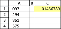
I have question, in range A1,A2,A3,A4 contain 097 494 861 575.
What is the formula in excel if the result that i want is 01456789
thanks
This formula contains two functions that are only available for Excel subscribers. This formula will not work in earlier Excel versions.
Update 8/26/2021 - Smaller formula:
3.1 Explaining formula in cell E2
Step 1 - Find search values in cell range
The SEARCH function allows you to search cell values and if a given text string is found a number is returned which represents the character position.
SEARCH(find_text, within_text, [start_num])
For example if 1 is returned the cell value begins with the text string.
The great thing about the SEARCH function is that it lets you search for multiple text strings, this makes the function return an array of numbers instead of a single number.
SEARCH({0, 1, 2, 3, 4, 5, 6, 7, 8, 9}, B3:B6)
returns {1, #VALUE!, ... , #VALUE!}
The comma is a column delimiting character and the semicolon is a row delimiting character, if I enter the above array in cell C3 the formula expands automatically to cell range C3:L6. This is called spilling and is a new Excel 365 feature.

The image above shows the find_text argument in row 2, the within_text in column B and the array in cell range C3:L6. Number 0 is found in the first value 097 in character position 1.
Step 2 - Identify non-error values
The ISNUMBER function lets you check if a cell value is a number, it returns the boolean value TRUE if a number and FALSE for everything else even error values.
ISNUMBER(SEARCH({0, 1, 2, 3, 4, 5, 6, 7, 8, 9}, B3:B6))
returns {TRUE, FALSE, ... , FALSE}

This step is required, the MMULT function, which we will use in step 4, can't process error values.
Step 3 - Convert boolean values to their numerical equivalents
Boolean value TRUE is the same thing as 1 and FALSE is 0 (zero). It is easy to convert boolean values simply multiply with 1.
ISNUMBER(SEARCH({0, 1, 2, 3, 4, 5, 6, 7, 8, 9}, B3:B6))*1
returns {1, 0, ... , 0}

Step 4 - Merge values column-wise using OR logic
The MMULT function is a capable of aplying OR logic for each column, the result is an array shown in row 7 in the image below.
MMULT(TRANSPOSE(ROW(B3:B6)^0), ISNUMBER(SEARCH({0, 1, 2, 3, 4, 5, 6, 7, 8, 9}, B3:B6))*1)
returns {1, 1, 0, 0, 1, 1, 1, 2, 1, 2}

Step 5 - Replace array values
The IF function returns one value if the logical expression evaluates to True and another value if False, this applies to an array of values as well.
IF(MMULT(TRANSPOSE(ROW(B3:B6)^0), ISNUMBER(SEARCH({0, 1, 2, 3, 4, 5, 6, 7, 8, 9}, B3:B6))*1), {0, 1, 2, 3, 4, 5, 6, 7, 8, 9}, "")
returns {0,1,"","",4,5,6,7,8,9}

The image above shows the following array {0,1,"","",4,5,6,7,8,9} in row 7. It tells you that number two and three are not in cell range C3:C6.
Step 6 - Concatenate array values
The TEXTJOIN function is self-explanatory it joins values and is capable of ignoring blank values with any given delimiting character or string.
TEXTJOIN(delimiter, ignore_empty, text1, [text2], ...)
TEXTJOIN("", TRUE, IF(MMULT(TRANSPOSE(ROW(B3:B6)^0), ISNUMBER(SEARCH({0, 1, 2, 3, 4, 5, 6, 7, 8, 9}, B3:B6))*1), {0, 1, 2, 3, 4, 5, 6, 7, 8, 9}, ""))
becomes
TEXTJOIN("", TRUE, {0,1,"","",4,5,6,7,8,9})
and returns "01456789".
Step 7 - Shorter formula
The LET function allows you to write shorter formulas by referring to names that contain a repeated expression. Our formula uses this array {0, 1, 2, 3, 4, 5, 6, 7, 8, 9} twice, we can use the LET function and name the array in order to simplify the formula.
LET(name1, name_value1, calculation_or_name2, [name_value2, calculation_or_name3...])
I named the array x and used x in two locations in the formula. This shortens the formula by 17 characters.
LET(x, {0, 1, 2, 3, 4, 5, 6, 7, 8, 9}, TEXTJOIN("", TRUE, IF(MMULT(TRANSPOSE(ROW(B3:B6)^0), ISNUMBER(SEARCH(x, B3:B6))*1), x, "")))
returns "01456789" in cell E2.
Will this formula work with blanks?

Yes, it works fine with blank cells in column B.
Can I mix text and numbers in column B?

Yes, the formula ignores letters and other characters.
Can I use values across columns?
No, the formula breaks if you try a multicolumn cell range like B3:C6.
4. Extract numbers from a column
The steps below demonstrate how to select only numbers from cell range B3:B12 manually. This means that you will be shown how to select cells containing only numbers and then copy the selection to a new cell range. Excel
You don't need to select all cells containing numbers one by one, this trick will save you a lot of time.
- Select cell range B3:B12 with your mouse.
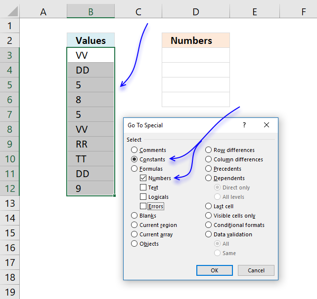
- Press function key F5 on your keyboard.
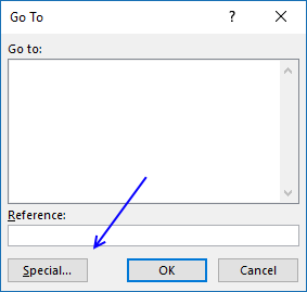
- A dialog box appears, press with left mouse button on "Special..." button.
- Another dialog box shows up, press with left mouse button on "Constants".
Note, if your selection contains formula then press with left mouse button on "Formulas".
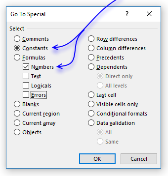
- Make sure checkbox "Numbers" is selected only, see image above.
- Press with left mouse button on OK button.
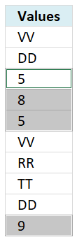
- The selection changes to only selecting numbers, see image above.
- Copy these cells. (CTRL + c)
- Select a destination cell with your mouse.
- Paste selection. (Ctrl + v)
The image below demonstrates an array formula that extracts numbers only, this can be useful in a dashboard or interactive worksheets.
The "Go to Special" dialog box in Microsoft Excel is a useful tool that allows you to quickly select specific types of cells or data within a worksheet. Here are some of the main things you can do with the "Go to Special" dialog box:
- Select Specific Cell Types:
- Blanks - Selects all the blank cells in the selected range.
- Constants - Selects all the cells containing constant values (not formulas).
- Formulas - Selects all the cells containing formulas.
- Numbers - Selects all the cells containing numeric values.
- Text - Selects all the cells containing text.
- Errors - Selects all the cells containing error values (e.g., #DIV/0!, #N/A, etc.).
- Select Unique Values:
- Unique - Selects all the unique values in the selected range.
- Duplicate - Selects all the duplicate values in the selected range.
- Select Conditional Formatting:
- Conditional Formats - Selects all the cells with conditional formatting applied.
- Select Data Validation:
- Data Validation - Selects all the cells with data validation rules applied.
- Select Hyperlinks:
- Hyperlinks - Selects all the cells containing hyperlinks.
- Select Commented Cells:
- Comments - Selects all the cells with comments.
The "Go to Special" dialog box can be particularly useful when you need to quickly identify and work with specific types of cells or data within a large worksheet. It can save time and make your data analysis and manipulation tasks more efficient.
5. Extract numbers from a column - Excel 365
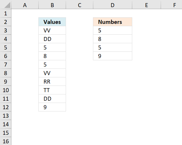
This section shows how to list cells containing numbers and only numbers. The image above shows source values in cell range B3:B12, they are VV, DD, 5, 8, 5, VV, RR, TT, DD, and 9. The formula in cell D3 lists values from B3:B12 that are identified as numbers meaning Excel interprets the value to be of a data type equal to a number.
Excel 365 formula in cell D3:
The formula in cell D3 returns 5, 8, 5, and 9 which are all numbers obviously. The output is an array that spills to cells below as far as needed. The formula utilizes two functions:
- ISNUMBER function which is a function that works in most Excel versions.
- FILTER function is a fairly new function available to only Excel 365 subscribers. This function is a dynamic array formula meaning it may return an array that spills top cells below.
Explaining formula
Step 1 - Identify numbers
The ISNUMBER function checks if a value is a number, returns TRUE or FALSE.
Function syntax: ISNUMBER(value)
ISNUMBER(B3:B12)
returns {FALSE; FALSE; TRUE; ... ; TRUE}.
Step 2 - Filter numbers
The FILTER function extracts values/rows based on a condition or criteria.
Function syntax: FILTER(array, include, [if_empty])
FILTER(B3:B12, ISNUMBER(B3:B12))
returns {5; 8; 5; 9}.
6. Extract numbers from a column - earlier Excel versions
If you have both letters and digits in a cell then read this article:
How to extract numbers from a cell value
Array formula in C2:
To enter an array formula, type the formula in a cell then press and hold CTRL + SHIFT simultaneously, now press Enter once. Release all keys.
The formula bar now shows the formula with a beginning and ending curly bracket telling you that you entered the formula successfully. Don't enter the curly brackets yourself.
Explaining formula in cell D3
Step 1 - Check if a value is a number
The ISNUMBER function returns TRUE if value is a number.
ISNUMBER($B$3:$B$12)
returns {FALSE; FALSE; TRUE; ... ; TRUE}
Step 2 - Convert TRUE to corresponding row number
The IF function returns corresponding row number if the logical test is TRUE and nothing "" if the logical test is FALSE.
IF(ISNUMBER($B$3:$B$12), ROW($B$3:$B$12)-MIN(ROW($B$3:$B$12))+1, "")
returns {""; ""; 3; ... ; 10}
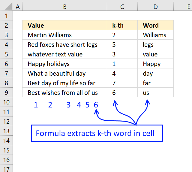
Step 3 - Return k-th smallest row number
The SMALL function makes sure that a new value is returned in each cell.
SMALL(IF(ISNUMBER($B$3:$B$12), ROW($B$3:$B$12)-MIN(ROW($B$3:$B$12))+1, ""), ROWS(D2:$D$2))
returns 3.
Step 4 - Return value
The INDEX function returns a value based on a row and column number.
INDEX($B$3:$B$12, SMALL(IF(ISNUMBER($B$3:$B$12), ROW($B$3:$B$12)-MIN(ROW($B$3:$B$12))+1, ""), ROWS(D2:$D$2)))
returns 5 in cell D3.
7. How to remove numbers from a cell value (Excel 2016)
The following formula contains the TEXTJOIN function and it works only in Excel 2016.
It allows you to filter values up to 1000 characters and you can easily change that limit by changing this cell reference: $A$1:$A$1000 in the formula above.
Explaining the Excel 2016 array formula in cell C3
Step 1 - Count characters in cell B3
The LEN function returns the number of characters in a cell value.
LEN(text)
LEN(B3)
becomes
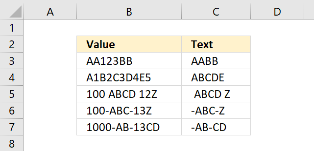
LEN("AA123BB")
and returns 7.
Step 2 - Create a reference
The INDEX function returns a value based on a row and column number (optional), however, it can also be used to create a dynamic cell reference.
INDEX($A$1:$A$1000, LEN(B3))
becomes
INDEX($A$1:$A$1000, 7)
and returns A7.
Step 3 - Create a cell reference to a cell range
$A$1:INDEX($A$1:$A$1000, LEN(B3))
becomes
$A$1:A7
Step 4 - Create row numbers based on cell ref
The ROW function returns a number representing the row number of a given cell reference.
ROW($A$1:INDEX($A$1:$A$1000, LEN(B3)))
becomes
ROW(A1:A7)
and returns
{1; 2; 3; 4; 5; 6; 7}.
Step 5 - Split characters in cell B3
The MID function returns a substring from a string based on the starting position and the number of characters you want to extract.
MID(text, start_num, num_chars)
MID(B3, ROW($A$1:INDEX($A$1:$A$1000, LEN(B3))), 1)
becomes
MID("AA123BB", {1; 2; 3; 4; 5; 6; 7}, 1)
and returns
{"A"; "A"; "1"; "2"; "3"; "B"; "B"}.
Step 6 - Remove numbers from array
The TEXT function lets you apply formatting to a given value.
TEXT(value, format_text)
TEXT(MID(B3, ROW($A$1:INDEX($A$1:$A$1000, LEN(B3))), 1), "")
becomes
TEXT({"A"; "A"; "1"; "2"; "3"; "B"; "B"}, "")
and returns
{"A"; "A"; ""; ""; ""; "B"; "B"}.
Step 7 - Join remaining characters
The TEXTJOIN function concatenates values in a cell range or array.
TEXTJOIN(delimiter, ignore_empty, text1, [text2], ...)
TEXTJOIN("", TRUE, TEXT(MID(B3, ROW($A$1:INDEX($A$1:$A$1000, LEN(B3))), 1), ""))
becomes
TEXTJOIN("", TRUE, {"A"; "A"; ""; ""; ""; "B"; "B"})
and returns "AABB".
8. How to remove numbers from a cell value - Excel 365
Update 1/12/2021 new dynamic array formula in cell C3:
This formula works only with Excel 365, it contains the new SEQUENCE function that creates an array containing numbers from 1 to n.
7.1 Explaining the Excel 365 dynamic array formula in cell C3
Step 1 - Count characters in cell B3
The LEN function returns the number of characters in a cell value.
LEN(text)
LEN(B3)
becomes
LEN("AA123BB")
and returns 7.
Step 2 - Create an array of numbers from 1 to n
The SEQUENCE fucntion creates a list of sequential numbers to a cell range or array. It is located in the Math and trigonometry category and is only available to Excel 365 subscribers.
SEQUENCE(rows, [columns], [start], [step])
SEQUENCE(LEN(B3))
becomes
SEQUENCE(7)
and returns
{1; 2; 3; 4; 5; 6; 7}.
Step 3 - Split value into characters
The MID function returns a substring from a string based on the starting position and the number of characters you want to extract.
MID(text, start_num, num_chars)
MID(B3, SEQUENCE(LEN(B3)), 1)
becomes
MID("AA123BB", {1; 2; 3; 4; 5; 6; 7}, 1)
and returns
{"A"; "A"; "1"; "2"; "3"; "B"; "B"}.
Step 4 - Remove numbers in the array
The TEXT function lets you apply formatting to a given value.
TEXT(value, format_text)
TEXT(MID(B3, SEQUENCE(LEN(B3)), 1), "")
becomes
TEXT({"A"; "A"; "1"; "2"; "3"; "B"; "B"}, "")
and returns
{"A"; "A"; ""; ""; ""; "B"; "B"}.
Step 5 - Join remaining characters
The TEXTJOIN function concatenates values in a cell range or array.
TEXTJOIN(delimiter, ignore_empty, text1, [text2], ...)
TEXTJOIN("", TRUE, TEXT(MID(B3, SEQUENCE(LEN(B3)), 1), ""))
becomes
TEXTJOIN("", TRUE, {"A"; "A"; ""; ""; ""; "B"; "B"})
and returns "AABB".
Get Excel *.xlsx file
How to remove numbers from cell value.xlsx
9. How to format numbers as text
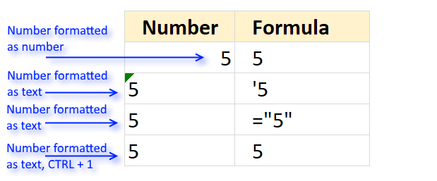
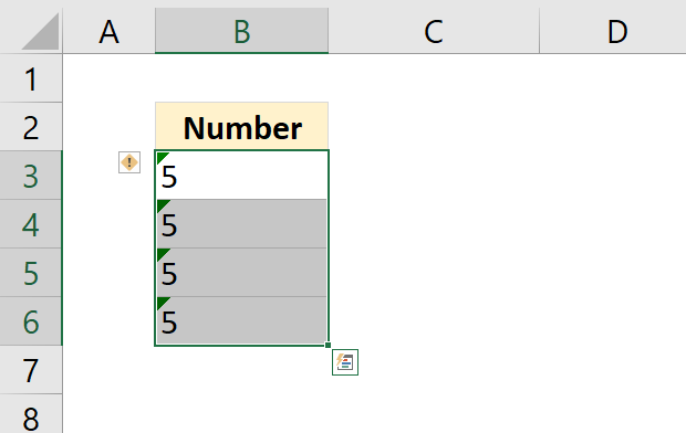
A number that is formatted as text will be left-aligned instead of right-aligned, this makes it easier for you to spot numbers that have been incorrectly formatted as text values.
The first example shows how Excel shows a number formatted as a number. The number is aligned to the right whereas numbers formatted as text are aligned to the left in the cell.
Method 1
Instructions:
- Select a cell
- Type '
- Type the number
- Press Enter
This example is shown in the second row in the image above.
Method 2
Instructions:
- Select a cell
- Type ="number"
- Press Enter
The number is the number you want to be formatted as text. This example is shown in the third row in the image above.
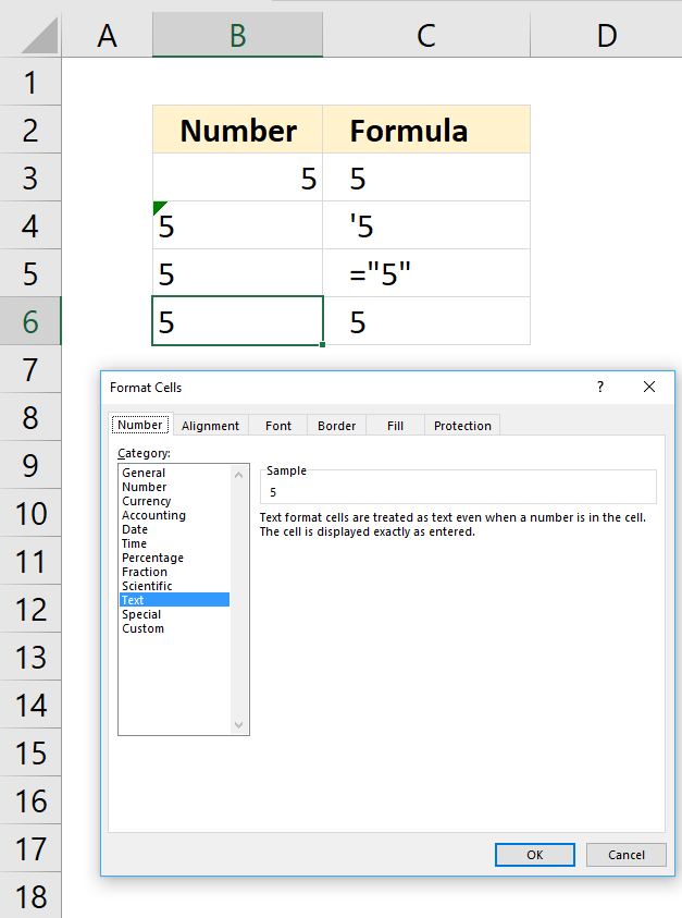
Method 3
Instructions:
- Select a cell
- Type the number
- Press Enter
- Press CTRL + 1 to open the "Format Cells" dialog box.
- Make sure you are on tab "Number".
- Select Category: "Text".
- Press with left mouse button on OK button.
Number incorrectly formatted as a text value
A green arrow appears in the upper left corner of the cell if Excel believes you have a number in your worksheet that was formatted incorrectly as text.
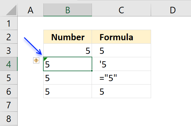
Press with left mouse button on the exclamation button and an options menu appears.
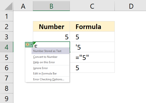
This lets you quickly deal with the problem:
| Convert to Number | Changes the formatting to a number. Value is now right-aligned. |
| Help on this Error | Opens a help guide inside Excel. |
| Ignore Error | Removes the green arrow, everything else remains as it is. |
| Edit in formula Bar | The prompt is moved to the formula bar where you can edit the cell value. |
| Error Checking Options... | Opens the "Excel Options" dialog box, see picture below. This allows you to change how Excel behaves when it comes to error values. |
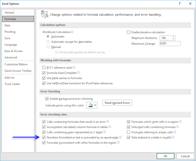
If you have multiple values checked as errors you can easily remove the green arrows by selecting the cells containing the error arrow. Then press with left mouse button on the "Exclamation mark" button and lastly press with left mouse button on "Ignore error".
Extract category
Whether you're cleaning up imported data, parsing product names, or building dynamic spreadsheets, mastering text manipulation in Excel can save […]
Excel categories
9 Responses to “How to extract numbers from a cell value”
Leave a Reply
How to comment
How to add a formula to your comment
<code>Insert your formula here.</code>
Convert less than and larger than signs
Use html character entities instead of less than and larger than signs.
< becomes < and > becomes >
How to add VBA code to your comment
[vb 1="vbnet" language=","]
Put your VBA code here.
[/vb]
How to add a picture to your comment:
Upload picture to postimage.org or imgur
Paste image link to your comment.
You could always use the brute force method (which eliminates the need for any helper cells)...
=IF(COUNTIF(A1:A4,"*0*"), 0, "")&IF(COUNTIF(A1:A4, "*1*"), 1, "")&IF(COUNTIF(A1:A4, "*2*"), 2, "")&IF(COUNTIF(A1:A4, "*3*"), 3, "")&IF(COUNTIF(A1:A4, "*4*"), 4, "")&IF(COUNTIF(A1:A4, "*5*"), 5, "")&IF(COUNTIF(A1:A4,"*6*"), 6, "")&IF(COUNTIF(A1:A4, "*7*"), 7, "")&IF(COUNTIF(A1:A4, "*8*"), 8, "")&IF(COUNTIF(A1:A4, "*9*"), 9, "")
And for the VBA code fans out there, one could use this UDF (user defined function)...
Function UniqueDigits(Rng As Range) As String Dim X As Long, Digits As String Digits = "0123456789" For X = 0 To 9 If Application.CountIf(Rng, "*" & X & "*") = 0 Then Mid(Digits, X + 1) = " " Next UniqueDigits = Replace(Digits, " ", "") End FunctionRick Rothstein (MVP - Excel),
Thank you for commenting.
Rick,
For me it's not working your formula (and UDF).
@Matt,
Just a guess, but your cells need to be formatted as Text before you enter the numbers into the cells or, alternately, enter your numbers into the cells preceded by an apostrophe (in order to make Excel see them as Text).
Can you bring unique within a single cell
mahmoud-lee,
See Rick Rothstein's formula.
similar Matrix solution but i think it's easier to explain, even if it feels inefficient: It Uses the "new" CONCAT instead of TEXTJOIN (Formula translated to English with VBA. It might work...)
=CONCAT(IFERROR(MID(A1,ROW(1:1000),1)*1,""))*1and with dynamic lenght
=CONCAT(IFERROR(MID(A1,ROW(INDIRECT("1:"&LEN(A1))),1)*1,""))*1A. Nony Mous
Thank you for your comment.
=CONCAT(IFERROR(MID(A1,ROW(1:1000),1)*1,""))*1
Your formula is a better, shorter and easier to understand.
Gracias por compartir, es la mejor solución que he encontrado en internet, además, muy bien explicada paso por paso. ¡Un 10!