Compatibility Functions

Table of Contents
- How to use the BETADIST function
- How to use the BETAINV function
- How to use the BINOMDIST function
- How to use the CHIDIST function
- How to use the CHIINV function
- How to use the CHITEST function
- How to use the CONFIDENCE functionartif
- How to use the COVAR function
- How to use the CRITBINOM function
- How to use the EXPONDIST function
- How to use the FDIST function
- How to use the FLOOR function
- How to use the FORECAST function
- How to use the FTEST function
- How to use the GAMMADIST function
- How to use the LOGNORMDIST function
- How to use the MODE function
- How to use the PERCENTRANK function
- How to use the QUARTILE function
- How to use the RANK function
- How to use the STDEV function
1. How to use the BETADIST function
What is the BETADIST function?
The BETADIST function calculates the cumulative beta distribution function representing an outcome in the form of probability.
What is the beta distribution?
The beta distribution is a continuous probability distribution defined over the interval [0, 1] and parameterized by two positive shape parameters, alpha (α) and beta (β).
What is a continuous probability distribution?
A continuous probability distribution is a function defined over a range of continuous values that provides the probability of a random variable falling between any two points, having a density described by an equation rather than discrete probabilities.
1.1 Syntax
BETADIST(x,alpha,beta,[A],[B])
1.2 Arguments
| x | Required. |
| alpha | Required. A parameter which determines the shape of the distribution. |
| beta | Required. A parameter which determines the shape of the distribution. |
| [A] | Optional. Lower bound, default value 0 (zero). |
| [B] | Optional. Upper bound, default value 1. |
What is a cumulative beta probability distribution?
The cumulative beta distribution function gives the probability that a beta-distributed random variable with parameters α and β will be less than or equal to a given value x, providing the accumulated area under the probability density curve from 0 to x.
When to use the beta distribution?
The beta distribution is used to model random variables limited to intervals of 0 to 1, such as binomial success probabilities, percentage or fraction outcomes, and measurements constrained between limits, making it useful in Bayesian statistics, experimental design, quality control studies, process monitoring, and other applications involving binary or fraction outcomes.
What are continuous values?
Continuous values are numbers that can take on any quantity within a range and can have infinitely many possibilities, unlike discrete values which have distinct separated values; continuous values can use intervals and ranges to describe events rather than fixed outcomes.
What are discrete probabilities?
Discrete probabilities are individual separated probabilities assigned to each of a countable number of possible outcomes that sum to 1, like rolling a die where each number has its own exact probability, as opposed to continuous distributions.
What are binomial success probabilities?
Binomial success probabilities describe the chance of a certain number of “successes” occurring in a fixed number of independent binary trial events modeled by the binomial distribution, like the probability of getting 3 heads in 10 coin flips.
What is Bayesian statistics?
Bayesian statistics is an approach to statistics using Bayes' theorem where prior beliefs about probabilities are updated as new evidence is acquired to determine conditional probabilities and update understanding of likelihood.
1.3 Example 1

The BETADIST function calculates the cumulative beta distribution representing an outcome in the form of probability between 0 and 1. The beta distribution is often used to model the uncertainty about the value of a probability or proportion when there is some prior information available.
Alpha is the number of successes plus one and beta is the number of failures plus one. Successes and failures is a generalization, it can be satisfied customers vs not satisfied customers or what ever you want.
A company manufactures a new product. The first 10 products has 7 working and 3 faulty. Assuming that the proportion of working products follows a beta distribution with parameters α = 8 and β = 4, what is the probability that more than 90% are working for the next products in line?
Alpha is the number of working products plus one and beta is the number of faulty products plus one. The ratio between the number of working products and the total number of products is 7/10 equals 0.7 The blue line has it's highest point at 0.7 if you check the x-axis.
The image above has argument
- x in cell C18 and that value is 0.9
- alpha in cell C19
- beta in cell C20
Formula in cell C24:
The formula in cell C24 returns approx. 0.981 which is the cumulative beta distribution meaning the area below the blue density probability function in the chart above up to x value 0.9
The value we are looking for is the area to the right of 0.9 which we can calculate by subtracting 0.947 with 1. 1 - 0.947 equals approx. 0.0185 or 1.85%
The probability that more than 90% are working is 1.85% The orange line in the chart displayed in the image above shows the cumulative value. As time goes by and more and more products are manufactured you can update the parameters of the beta distribution model to get a better probability value.
1.4 Example 2

This example continues on example 1 above. The company has now manufactured 100 products, 90 working and 10 defect.
The BETADIST function returns approx 0.570 which gives us 1 - 0.570 equals 0.430 or 43 %. This number 43% is the probability that the products to be manufactured in the future have 90% working and 10% defect.
This example shows that as the number of observations increases the probability density curve (blue) gets more narrow meaning the uncertainty is also decreasing. In other words, the function gets better at predicting the probability as the number of observations increases.
1.5 Example 3
The optional arguments [A] and [B] are lower and upper limits. The BETADIST function uses these limits to calculate the percentage value, a number between 0 and 1.
You will get the same result if you calculate the percentage yourself, here is an example.
The arguments are:
- x = 30
- alpha = 90
- beta = 110
- [A] = 15
- [B] = 45
Formula in cell C7:
The formula in cell C7 returns 0.922 which is 92.2 %. To calculate the percentage (x) we calculate the ratio between x and the total of the upper and lower limit.
30/(15+45) equals 30/60 = 0.5 We can use this number in the BETADIST function without the upper and lower limit and check if we get the same result.
=BETADIST(0.5,90,110)
returns 0.921957262116145 which is the exact same value as above (0.921957262116145).
1.6 Function not working
The BETADIST function returns
- #VALUE! error value if any argument is non-numeric.
- #NUM! error value if:
- alpha <= 0
- beta <= 0
- x < A
- x >B
- A = B
1.7 How is the function calculated?
The general equation to calculate the beta distribution:
2. How to use the BETAINV function
What is the BETAINV function?
The BETAINV function calculates the inverse of a cumulative beta distribution. The beta distribution can help estimate how long a project might take by using the expected finish time and how variable the timeline could be. It gives the chance the project will be done at different dates based on the variability.
This function is outdated and replaced by the BETA.INV function which was introduced in Excel 2010.
The BETAINV function may not be available in future Excel versions and Microsoft recommends using the newer function from now on.
What is the inverse of the cumulative beta distribution?
The inverse of the cumulative beta distribution is a function that returns the value of x for a given probability p and parameters α and β of the beta distribution.
What is a cumulative beta probability distribution?
The cumulative beta distribution function gives the probability that a beta-distributed random variable with parameters α and β will be less than or equal to a given value x, providing the accumulated area under the probability density curve from 0 to x.
What is a beta probability density distribution?
A beta probability density distribution is a function whose shape over [0,1] depends on parameters α and β that gives the relative likelihood of a beta-distributed random variable occurring at different points, whose total area under the curve integrates to 1.
What are continuous values?
Continuous values are numbers that can take on any quantity within a range and can have infinitely many possibilities, unlike discrete values which have distinct separated values; continuous values can use intervals and ranges to describe events rather than fixed outcomes.
What are discrete probabilities?
Discrete probabilities are individual separated probabilities assigned to each of a countable number of possible outcomes that sum to 1, like rolling a die where each number has its own exact probability, as opposed to continuous distributions.
What are binomial success probabilities?
Binomial success probabilities describe the chance of a certain number of “successes” occurring in a fixed number of independent binary trial events modeled by the binomial distribution, like the probability of getting 3 heads in 10 coin flips.
What is Bayesian statistics?
Bayesian statistics is an approach to statistics using Bayes' theorem where prior beliefs about probabilities are updated as new evidence is acquired to determine conditional probabilities and update understanding of likelihood.
2.1 Syntax
BETAINV(probability,alpha,beta,[A],[B])
2.2 Arguments
| probability | Required. |
| alpha | Required. A parameter which determines the shape of the distribution. |
| beta | Required. A parameter which determines the shape of the distribution. |
| [A] | Optional. Lower bound, default value 0 (zero). |
| [B] | Optional. Upper bound, default value 1. |
What is alpha and beta in a beta distribution?
The beta distribution is very flexible due to how alpha and beta shape its variance and skew. Changing their values gives a wide range of distribution shapes. In the beta distribution, alpha and beta are shape parameters that control the form of the distribution:
Alpha (α): Controls the height of the peak. Higher alpha = taller, more concentrated peak. Alpha mainly changes the peak height.
Beta (β): Controls the tails of the distribution. Higher beta = shorter, thinner tails. Beta mainly changes the tail thickness.
As α & β > 1, shape becomes more symmetric and bell-shaped.
As α & β < 1, shape becomes asymmetrical and J or U shaped.
When α = β = 1, the distribution becomes uniform.
They allow modeling different levels of variance and asymmetry.
2.3 Example 1

The BETAINV function calculates the inverse of the cumulative beta distribution representing an outcome in the form of probability between 0 and 1.
The BETADIST function is related to the BETAINV function: BETAINV(probability,alpha,beta,[A],[B]) = x
BETADIST(x,alpha,beta,[A],[B]) = probability
A company manufactures a new product. The first 10 products has 7 working and 3 faulty. Assuming that the proportion of working products follows a beta distribution with parameters α = 8 and β = 4, find the values of the proportion corresponding to the 2.5th and 97.5th percentiles?
Alpha is the number of working products plus one and beta is the number of faulty products plus one. The ratio between the number of working products and the total number of products is 7/10 equals 0.7 The blue line has it's highest point at 0.7 if you check the x-axis.
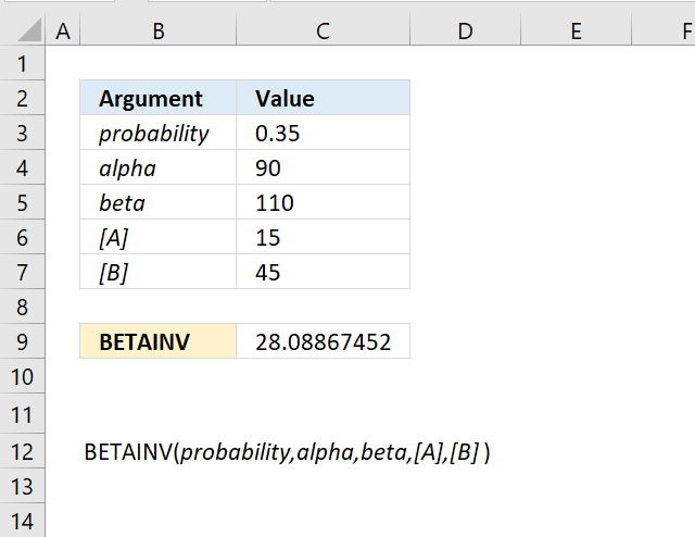
The image above has argument
- probability in cell C18 and that value is 0.975
- alpha in cell C19
- beta in cell C20
Formula in cell C10:
The formula returns approx. 0.891 for a probability of 97.5% and approx. 0.390 for a probability of 2.5%.
2.4 Example 2

This example continues on example 1 above. The company has now manufactured 100 products, 90 working and 10 defect.
Assuming that the proportion of working products follows a beta distribution with parameters α = 91 and β = 11, find the values of the proportion corresponding to the 2.5th and 97.5th percentiles?
The BETAINV function returns 0.944 for 97.5% and 0.825 for 2.5 %.
This example shows that as the number of observations increases the probability density curve (blue) gets more narrow meaning the uncertainty is also decreasing. In other words, the function gets better as the number of observations increases.
2.5 Example 3

The optional arguments [A] and [B] are lower and upper limits respectively. The BETAINV function uses these limits to assist you calculating the x value for you which is a number between the lower limit and the upper limit.
You will get the same result if you calculate the x value yourself, here is an example.
The arguments are:
- probability = 0.921957262116145
- alpha = 90
- beta = 110
- [A] = 15
- [B] = 45
Formula in cell C7:
The formula in cell C7 returns 30.You can calculate x using only three arguments probability, alpha, and beta. Multiply the result with the total of the upper and lower limit to calculate x. It will be somewhere between the limits. Here is how:
=BETAINV(0.921957262116145,90,110)
returns 0.5
0.5*(15+45)=30 which is exactly what the function returns in cell C24
2.6 Function not working
The BETAINV function returns a:
- #VALUE! error value if any argument is non-numeric.
- #NUM! error value if:
- alpha <= 0 (zero)
- beta <= 0 (zero)
- probability <= 0 (zero)
- probability > 1
- A = B
3. How to use the BINOMDIST function

What is the BINOMDIST function?
The BINOMDIST function calculates the individual term binomial distribution probability, use this function when
- the success probability is constant through all trials
- you know the number of trials
- the outcome is either a success or failure
- each trial is independent of the other trials.
What is the binomial distribution probability?
The binomial distribution probability gives the likelihood of a specific number of successes occurring in a fixed number of independent trials, each having the same binary success/failure probability.
What is the individual term binomial distribution probability?
The individual term binomial distribution probability is the probability of exactly k successes in n trials with a given success probability p, calculated using combinations to determine the number of ways k successes can occur in those trials.
What are combinations?
A combination is a way of selecting items from a collection where the order of selection does not matter.
For example, if you have three fruits, say an apple, an orange, and a pear. There are three combinations of two that can be drawn from this set:
- apple and a pear
- apple and an orange
- pear and an orange
3.1 Syntax
BINOMDIST(number_s,trials,probability_s,cumulative)
3.2 Arguments
| number_s | Required. The number of successful tests. |
| trials | Required. How many independent tests. |
| probability_s | Required. The probability of success in each test. |
| cumulative | Required. A boolean value. TRUE - cumulative distribution function FALSE - probability mass function |
What is cumulative binomial distribution?
The cumulative binomial distribution function gives the probability that a binomial random variable with a given number of trials and success probability will take on a value less than or equal to a specified number of successes x.
What is probability mass function?
A probability mass function is a function that defines a discrete probability distribution by providing the probability that each of a countable number of possible discrete outcomes will occur for a random variable.
What is a binomial random variable?
A binomial random variable is a discrete random variable that represents the number of "successes" in a fixed number of independent binary trials, where each trial has the same probability of success.
What are discrete probabilities?
Discrete probabilities are individual separated probabilities assigned to each of a countable number of possible outcomes that sum to 1, like rolling a die where each number has its own exact probability, as opposed to continuous distributions.
3.3 Example 1
The probability that a customer accepts an offer is estimated to be 60%. The offer is given to 20 customers. What is the probability that at most 12 of them accepts the offer?
To solve this we need to use the binomial distribution. It models the number of successes in a fixed number of independent trials (20 customers). Each trial has the same probability of success (0.6 or 60%).
Let x be the random variable representing the number of customers who accepts the offer. Then x follows a binomial distribution with parameters n = 20 (number of trials) and p = 0.6 (probability of success).
The probability we want to find is P(x ≤ 12) which is the cumulative probability of the binomial distribution from 0 up to 12.
Formula in cell C8:
The formula returns approx. 0.5841, in other words, the probability is 58.4% that up to 12 customers accepts the offer.
The chart in the image above shows an orange line representing the cumulative probability. Go to 12 on the x-axis and find where the orange line intersects the middle of the column. The secondary y-axis to the right shows a value just below 0.6 which seems to match the calculated number 0.5841
3.4 Example 2

There are 22 machines that operate independently of each other in a factory. The probability of a breakdown occurring during a day is 0.1 for each of the machines. What is the probability that three machines will stop during a certain day?
The binomial distribution is what we need in this example. It models the number of successes (machine breakdowns) in a fixed number of independent trials (22 machines), where each trial has the same probability of success (0.1 or 10%).
Let x be the random variable representing the number of machines that break down during the day. Then x follows a binomial distribution with parameters n = 22 (number of machines) and p = 0.1 (probability of breakdown for each machine).
The probability we want to find is P(X = 3), which is the probability mass function of the binomial distribution evaluated at 3.
The formula returns 0.208, in other words, the probability is 20.8% that exactly 3 machines break down during a day.
The chart in the image above shows blue chart columns representing the probability mass function of the binomial distribution. Go to 3 on the x-axis and find the value value for that column. The y-axis to the left shows a value just above 0.2 which seems to match the calculated number 0.208
3.5 Example 3

There are 30 students in a class. There is a 50% risk that each student, independently of each other, will catch a harmless but highly contagious cold. What is the chance that 12 students or less will attend school on the same day?
We need to find the probability that 12 or fewer students will not catch the cold, which is the same as the probability that 18 or more students will catch the cold.
- Total number of students: 30
- Probability of catching the cold for each student: 0.5 (or 50%)
We want to find P(X ≥ 18), which is the probability that 18 or more students will catch the cold.
P(X ≥ 18) = 1 - P(X ≤ 17)
We can calculate P(X ≤ 17) using the cumulative distribution function of the binomial distribution and then take the complement to find P(X ≥ 18).
Formula in cell C21:
The formula in cell C21 returns 0.181 which is 18.1%. This means that there is a 18.1% chance that 12 students or less will attend school on the same day.
3.6 Function not working
The BINOMDIST function returns
- #VALUE! error value if number_s, trials or probability_s argument is non-numeric.
- #NUM! error value if:
- number_s <= 0 (zero)
- number_s > trials
- probability_s < 0 (zero)
- probability_s > 1
- A = B
number_s and trials are converted into integers.
4. How to use the CHIDIST function
The CHIDIST function calculates the right-tailed probability of the chi-squared distribution. Use this function to check if a hypothesize is valid.
What is a chi-squared distribution?
The chi-squared distribution is a theoretical probability distribution modeling the sum of squared standard normal random variables used in inferential statistics for estimation, confidence intervals, and hypothesis testing.
What is the probability of the chi-squared distribution?
The probability of the chi-squared distribution determines the likelihood that the sum of squared standard normal variables will take on a value less than or equal to a given number, depending on its degrees of freedom parameter.
What is a hypothesize?
In statistics, a hypothesis is an assumption about some aspect of a population parameter or probability model that can be tested using observations and data to determine if there is sufficient evidence in the sample to support the assumed hypothesis.
What is a cumulative chi-squared distribution?
The cumulative chi-squared distribution function gives the probability that the sum of squared standard normals will result in a value less than or equal to a specified number x, giving the accumulated area under the probability density curve.
What is a probability density function of a chi-squared distribution?
A chi-squared probability density function is a function that defines the relative likelihood of different outcomes for the sum of squared standard normals based on its degrees of freedom parameter, integrating to a total area of 1 over the domain.
What is inferential statistics for estimation?
Inferential statistics for estimation involve using a random sample to estimate characteristics and parameters about a larger population using statistical techniques like confidence intervals and point estimation to quantify uncertainty about the estimates.
What is confidence intervals?
A confidence interval provides a range of plausible values for an unknown population parameter centered around a sample estimate, describing the uncertainty around the estimate at a specified level of confidence.
What is the sum of squared standard normal variables?
The sum of squared standard normal variables refers to summing multiple independent normally distributed random variables each with a mean of 0 and variance of 1, which results in a chi-squared distribution that can be used for statistical modeling and analysis.
4.1 Syntax
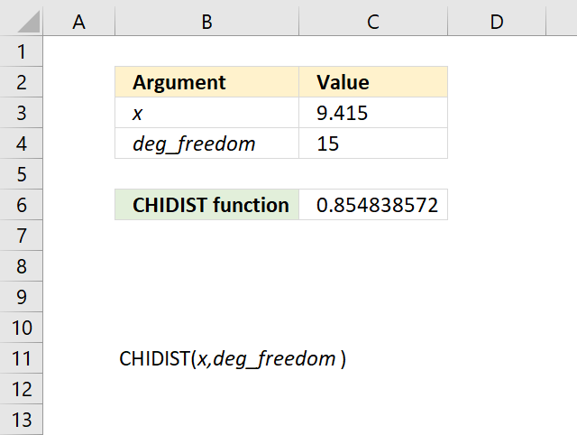
CHIDIST(x,deg_freedom)
4.2 Arguments
| x | Required. A numerical value representing a point in the probability distribution you want to be evaluated. |
| deg_freedom | Required. A numerical value representing the degrees of freedom. |
deg_freedom argument is converted into integers.
What are the degrees of freedom?
The degrees of freedom in a chi-squared distribution refers to the number of standard normal random variables being squared and summed, which affects the shape of the distribution and occurs in statistical tests as the sample size minus the number of estimated parameters.
What is a boolean value?
A Boolean value is a logical data type having only two possible states - true or false - which logic gates and circuits are based on.
4.3 Example 1

The CHIDIST function calculates the right-tailed probability of a given x value based on the chosen number of degrees of freedom. This means that the right-tailed probability represents the area below the orange line from a given x value to infinity.
For example, the image above shows a chart containing two lines colored blue and orange.
- Blue line - chi squared density probability function
- Orange line - cumulative chi-squared distribution
Both lines represents a chi-squared distribution with 1 degree of freedom. The formula in cell C20 contains the CHIDIST function, it calculates the probability based on the following arguments:
- x - 2
- deg_freedom - 1
Formula in cell C20:
=CHIDIST(C16,C17)
It returns 0.157299207050285 which represents the area below the orange line from x value = 2 and to infinity. You can also find that value if you find number 2 on the x-axis and then locates the value on the y-axis where x value 2 intersects the blue line which is somewhere around 0.85
0.85 is the left tailed cumulative probability for the chi squared distribution with 1 degree of freedom, however, the right-tailed probability is easy to calculate. We need to find the complement which we can calculate by subtracting 1 with 0.85 This results in 1 - 0.85 = 0.15 which is approx. 0.157299207050285
4.4 Example 2

What is the right-tailed probability for a chi-squared distribution with two degrees of freedom for an x value of 3?
The CHIDIST function has two arguments:
- x - which is specified in cell C16 and is 3 in this example.
- deg_freedom - The degree of freedom is 2 and is specified in cell C17.
The image above shows a chart demonstrating both the cumulative chi-squared distribution (blue line) and the density probability function (orange line) between x values of 0 to 10. These distribution lines change based on the degree of freedom value. In this example the two lines has 2 degrees of freedom.
Formula in cell C20:
The formula in cell C20 returns approx. 0.223. This value can be found in the chart above. First we need to calculate the complement to 0.223 which is 1- 0.223 = 0.777
The orange line shows the density probability function, the x value is found on the x-axis. 3 on the x-axis corresponds to the 0.777 value on the y-axis based on the intersection between the blue line and x value 3.
4.5. Example 3

What is the right-tailed probability for a chi-squared distribution with eight degrees of freedom for an x value of 6?
The CHIDIST function has two arguments:
- x - which is specified in cell C16 and is 6 in this example.
- deg_freedom - The degree of freedom is 8 and is specified in cell C17.
The image above shows a chart demonstrating both the cumulative chi-squared distribution (blue line) and the density probability function (orange line) between x values of 0 to 10. These distribution lines change based on the degree of freedom value. In this example the two lines has 8 degrees of freedom.
Formula in cell C20:
The formula in cell C20 returns approx. 0.65. This value can be found in the chart above. First we need to calculate the complement to 0.65 which is 1- 0.65 = 0.35
The orange line shows the density probability function, the x value is found on the x-axis. 6 on the x-axis corresponds to the 0.35 value on the y-axis based on the intersection between the blue line and x value 6.
4.6. Function not working
The CHIDIST function returns
- #VALUE! error value if x or deg_freedom argument is non-numeric.
- #NUM! error value if:
- x < 0 (zero)
- deg_freedom < 1
- deg_freedom > 10^10
5. How to use the CHIINV function

What is the CHIINV function?
The CHIINV function calculates the inverse of the right tailed probability of the chi-squared distribution.
What is a chi-squared distribution?
The chi-squared distribution is a theoretical probability distribution modeling the sum of squared standard normal random variables used in inferential statistics for estimation, confidence intervals, and hypothesis testing.
What is the probability of the chi-squared distribution?
The probability of the chi-squared distribution determines the likelihood that the sum of squared standard normal variables will take on a value less than or equal to a given number, depending on its degrees of freedom parameter.
What is a hypothesize?
In statistics, a hypothesis is an assumption about some aspect of a population parameter or probability model that can be tested using observations and data to determine if there is sufficient evidence in the sample to support the assumed hypothesis.
What is inferential statistics for estimation?
Inferential statistics for estimation involve using a random sample to estimate characteristics and parameters about a larger population using statistical techniques like confidence intervals and point estimation to quantify uncertainty about the estimates.
What is confidence intervals?
A confidence interval provides a range of plausible values for an unknown population parameter centered around a sample estimate, describing the uncertainty around the estimate at a specified level of confidence.
What is the left-tailed probability of the chi-squared distribution?
The left-tailed probability of the chi-squared distribution gives the chance that the sum of squared standard normals is less than or equal to a specified value x, focusing only on the lower portion of outcomes under the density curve.
What is the inverse of a left-tailed probability of the chi-squared distribution?
The inverse of a left-tailed chi-squared probability determines the value x that corresponds to a given cumulative probability for the lower tail, calculating the sum of squares threshold that captures the specified proportion of possible outcomes.
What is the difference between the CHIDIST and CHINV functions?
The CHIDIST and CHINV functions are related.
CHIDIST(x, deg_freedom) = probability
then
CHINV(probability , deg_freedom) = x
5.1 Syntax
CHIINV(probability,deg_freedom)
5.2 Arguments
| probability | Required. A numerical value representing the probability with the chi-squared distribution. |
| deg_freedom | Required. A numerical value representing the degrees of freedom. |
What are the degrees of freedom?
The degrees of freedom in a chi-squared distribution refers to the number of standard normal random variables being squared and summed, which affects the shape of the distribution and occurs in statistical tests as the sample size minus the number of estimated parameters.
5.3 Example 1
What is x for the right-tailed probability of 0.317310507862914 with 1 degree of freedom?
The image above shows a chart displaying the chi square distribution for a degree of freedom of 1. The blue line is the cumulative chi square distribution and the orange line is the density probability function.
Below the chart are the arguments specified:
- probability : 0.317310507862914
- deg_freedom : 1
The formula in cell C20 calculates the inverse (x) of the right-tailed probability of the chi-squared distribution based on the specified arguments above. This means the area below the orange line from x value = 1 to infinity.
Formula in cell C20:
This means that 0.317310507862914 represents the area below the orange line from x value = 1 to infinity.
0.317310507862914 is the right-tailed probability value, to calculate the left-tailed probability we need the complement. We subtract 1 with 0.317310507862914 which equals 0.682689492137086
We can now find the probability value (0.6827) on the y-axis, then find where the cumulative chi square distribution which is the blue line intersects 0.6827. Now find the x value on the x-axis which is 1 based on the intersection of the blue line and y-axis value 0.6827. This value matches the calculated value in cell C20.
Cell C21 contains the CHIDIST function, it calculates the right-tailed probability based on the calculated value in cell C20, the number of degrees of freedom specified in cell C17 which corresponds to the cumulative chi square distribution.
The value in cell C21 matches the value in cell C16 which demonstrates the relation between the CHIDIST function and the CHIINV function.
5.4 Example 2

What is x for the right-tailed probability of 0.22313016014843 with 2 degrees of freedom?
The image above shows a chart displaying the chi square distribution for 2 degrees of freedom. The blue line is the cumulative chi square distribution and the orange line is the density probability function.
Below the chart are the arguments specified:
- probability : 0.22313016014843
- deg_freedom : 2
The formula in cell C20 calculates the inverse (x) of the right-tailed probability of the chi-squared distribution based on the specified arguments above.
Formula in cell C20:
This means that 0.22313016014843 represents the area below the orange line from x value = 3 to infinity.
0.22313016014843 is the right-tailed probability value, to calculate the left-tailed probability we need the complement. We subtract 1 with 0.22313016014843 which equals 0.77686983985157
We can now find the probability value (0.7769) on the y-axis, then find where the cumulative chi square distribution which is the blue line intersects 0.7769. Now find the x value on the x-axis which is 3 based on the intersection of the blue line and y-axis value 0.7769. This value matches the calculated value in cell C20.
Cell C21 contains the CHIDIST function, it calculates the right-tailed probability based on the calculated value in cell C20, the number of degrees of freedom specified in cell C17 which corresponds to the cumulative chi square distribution.
The value in cell C21 matches the value in cell C16 which demonstrates the relation between the CHIDIST function and the CHIINV function.
5.5 Example 3

What is x for the right-tailed probability of 0.433470120366709 with 8 degrees of freedom?
The image above shows a chart displaying the chi square distribution for 8 degrees of freedom. The blue line is the cumulative chi square distribution and the orange line is the density probability function.
Below the chart are the arguments specified:
- probability : 0.433470120366709
- deg_freedom : 8
The formula in cell C20 calculates the inverse (x) of the right-tailed probability of the chi-squared distribution based on the specified arguments above.
Formula in cell C20:
This means that 0.433470120366709 represents the area below the orange line from x value = 8 to infinity.
0.22313016014843 is the right-tailed probability value, to calculate the left-tailed probability we need the complement. We subtract 1 with 0.22313016014843 which equals 0.77686983985157
We can now find the probability value (0.7769) on the y-axis, then find where the cumulative chi square distribution which is the blue line intersects 0.7769. Now find the x value on the x-axis which is 8 based on the intersection of the blue line and y-axis value 0.7769. This value matches the calculated value in cell C20.
Cell C21 contains the CHIDIST function, it calculates the right-tailed probability based on the calculated value in cell C20, the number of degrees of freedom specified in cell C17 which corresponds to the cumulative chi square distribution.
The value in cell C21 matches the value in cell C16 which demonstrates the relation between the CHIDIST function and the CHIINV function.
5.6. Function not working
The CHIINV function returns
- #VALUE! error value if probability or deg_freedom argument is non-numeric.
- #NUM! error value if:
- probability < 0 (zero)
- probability > 1 (zero)
- deg_freedom < 1
deg_freedom argument is converted into integers if necessary.
6. How to use the CHITEST function
The CHITEST function calculates the test for independence, the value returned from the chi-squared statistical distribution and the correct degrees of freedom. Use this function to check if hypothesized results are valid.
What is a test for independence?
A test for independence is a statistical hypothesis test that checks if two categorical variables are related or independent based on observed data, commonly done using Pearson's chi-squared test or G-test to compare observed and expected frequency counts.
What is a chi-squared distribution?
The chi-squared distribution is a theoretical probability distribution modeling the sum of squared standard normal random variables used in inferential statistics for estimation, confidence intervals, and hypothesis testing.
What is the probability of the chi-squared distribution?
The probability of the chi-squared distribution determines the likelihood that the sum of squared standard normal variables will take on a value less than or equal to a given number, depending on its degrees of freedom parameter.
What is an hypothesis?
In statistics, a hypothesis is an assumption about some aspect of a population parameter or probability model that can be tested using observations and data to determine if there is sufficient evidence in the sample to support the assumed hypothesis.
What is a cumulative chi-squared distribution?
The cumulative chi-squared distribution function gives the probability that the sum of squared standard normals will result in a value less than or equal to a specified number x, giving the accumulated area under the probability density curve.
What is a probability density function of a chi-squared distribution?
A chi-squared probability density function is a function that defines the relative likelihood of different outcomes for the sum of squared standard normals based on its degrees of freedom parameter, integrating to a total area of 1 over the domain.
What is inferential statistics for estimation?
Inferential statistics for estimation involve using a random sample to estimate characteristics and parameters about a larger population using statistical techniques like confidence intervals and point estimation to quantify uncertainty about the estimates.
What is confidence intervals?
A confidence interval provides a range of plausible values for an unknown population parameter centered around a sample estimate, describing the uncertainty around the estimate at a specified level of confidence.
What is the sum of squared standard normal variables?
The sum of squared standard normal variables refers to summing multiple independent normally distributed random variables each with a mean of 0 and variance of 1, which results in a chi-squared distribution that can be used for statistical modeling and analysis.
What are the degrees of freedom?
The degrees of freedom in a chi-squared distribution refers to the number of standard normal random variables being squared and summed, which affects the shape of the distribution and occurs in statistical tests as the sample size minus the number of estimated parameters.
6.1. Syntax
CHITEST(actual_range,expected_range)
6.2. Arguments
| actual_range | Required. A range of data. |
| expected_range | Required. A range of data. |
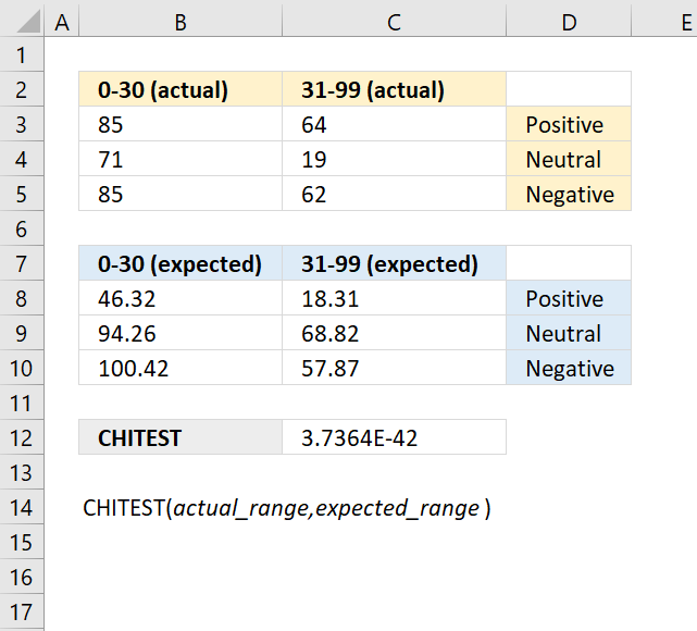
6.3. Example
How to check if hypothesized results are valid when using the CHISQ.TEST function?
To check if results from the CHISQ.TEST function are valid, look at the calculated test statistic and compare it to the critical value from the chi-squared distribution with degrees of freedom equal to (number of rows - 1) * (number of columns - 1) at the desired significance level, rejecting independence if the test statistic exceeds the critical value.
Formula in cell C12:
6.4. Example 2

In an archaeological study, researchers have collected data on the frequencies of different types of artifacts found at various excavation sites. They want to test if the observed frequencies of artifact types differ significantly from the expected frequencies based on historical records or theoretical models.
Observed frequencies of artifact types:
| Artifact types | Frequency: |
| A | 432 |
| B | 312 |
| C | 613 |
| D | 171 |
The theoretical probabilities for the artifacts are as follows:
| Artifact types | Probabilities |
| A | 0.25 |
| B | 0.18 |
| C | 0.41 |
| D | 0.16 |
Evaluate if the observed frequencies of artifact types deviate significantly from the expected frequencies.
Formula in cell C23:
Formula in cell D27:
Copy cell D27 to cells below as far as needed.
Formula in cell C32:
The CHISQ.TEST function returns 1.848E-07
Formula in cell C33:
Formula in cell C34:
The χ2 statistic for the observed frequencies is approx. 34.14 with 3 degrees of freedom. This is higher than the decision rule calculated in cell C34. The observed frequencies does differ significantly from the expected frequencies.
6.5. Function not working
Independence is indicated by a low number of χ2.
The CHITEST function returns
- #N/A error value if the number of data points in the arguments doesn't match.
6.6. How is the CHITEST Function calculated?
CHITEST function equation:
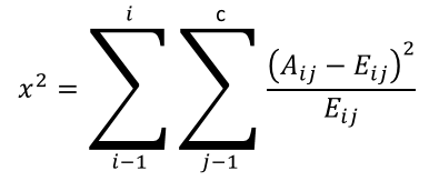
Aij = actual frequency in the i-th row, j-th column
Eij = expected frequency in the i-th row, j-th column
r = number of rows
c = number of columns
7. How to use the CONFIDENCE function

What is the CONFIDENCE function?
The CONFIDENCE function calculates the confidence interval for a population mean, using a normal distribution.
There are newer better functions that may have improved accuracy, this function is available for compatibility with older workbooks created in earlier Excel versions and other older software.
The new CONFIDENCE.NORM function and the CONFIDENCE.T function replace the older CONFIDENCE function which have better accuracy and improved functionality, Microsoft informs that the CONFIDENCE function may not be available in future Excel versions and recommends using the CONFIDENCE.NORM or the CONFIDENCE.T from now on.
What is a confidence interval?
A confidence interval is a range of values used to estimate a population parameter based on a sample statistic. It is constructed using a point estimate (such as the sample mean) plus or minus a margin of error.
The confidence level indicates the probability that the true population parameter lies within the interval. 90%, 95% and 99% confidence levels are commonly used. Useful for quantifying the uncertainty and potential error in statistics, surveys, polls, etc.
What is a population sample?
A population sample in statistics refers to a subset of data points selected from a larger population. The sample is a portion drawn from the total population.
It is studied to make inferences about the whole population, a sample aims to represent the population characteristics. The sample should be chosen randomly when possible to avoid bias.
The sample size should be adequate to represent the population, larger samples produce more precise results. Sampling reduces the cost and effort of studying the entire population and results are subject to sampling error due to studying a subset only.
How to pick a sample size to represent the population?
A typical starting point is to sample 5-10% of a large population or 20-30% of a small population. Statistical equations using confidence level, margin of error, and variance can precisely calculate the optimal sample size.
The goal is to pick a sample size large enough to produce a reasonable margin of error and desired power at a given confidence level. Higher confidence in the results requires a larger sample. Common levels are 90%, 95%, 99%.
The amount of potential error tolerated in results. Lower margin needs a larger sample. Larger populations require a bigger sample. Smaller populations need a higher sampling percentage. Bigger samples require more time, money and effort. Need to balance accuracy and feasibility.
What is a population mean?
The population mean is the average value of a quantitative variable calculated across an entire population also called the expected value or population average.
It is calculated by summing all the values in the population and dividing by the total number of individuals and is represented by the Greek letter μ (mu).
What is a normal distribution?

The normal distribution is a symmetric bell-shaped probability distribution described by its mean and standard deviation. Used by many to model a plethora of natural phenomena and represent unknown processes.
7.1. Syntax
CONFIDENCE(alpha, standard_dev, size)
7.2. Arguments
| alpha | Required. The significance level used to calculate the confidence level. 0.05 represents a 95% confidence level. |
| standard_dev | Required. The standard deviation for the data points. |
| size | Required. The number of data points. |
7.3. Example 1
A quality control manager at a manufacturing plant wants to determine the acceptable range of tensile strengths for a particular type of steel cable. They have recorded the tensile strengths of 25 randomly selected steel cable samples. Calculate the 90% confidence interval for the mean tensile strength of the steel cables.
The CONFIDENCE function lets you calculate the interval that satisfies a given a significance level, standard deviation and a number representing the population size.
The image above shows the argument:
- alpha in cell C19 which is 1-0.90 = 0.1
- standard_dev in cell C20 = 9.5
- size in cell C21 = 25
- Mean μ = 80
Formula in cell B6:
The CONFIDENCE function returns 3.1252218912078 for the specified arguments above.We can now calculate the upper and lower limit by adding the confidence interval from cell C23 to the mean μ. I have done this in cell C25:
The lower limit is calculated by subtracting the confidence level to the mean μ. Cell 26:
There is a 90% probability that the mean μ is between approx. 76.87 and approx. 83.13
7.4. Example 2

A researcher wants to estimate the average height of male students in a university. They take a random sample of 30 male students and measure their heights. Using the sample data, calculate the 95% confidence interval for the mean height of male students in the university.
Formula in cell B6:
The CONFIDENCE function lets you calculate the interval that satisfies a given a significance level, standard deviation and a number representing the population size.
The image above shows the argument:
- alpha in cell C19 which is 1-0.95 = 0.05
- standard_dev in cell C20 = 12
- size in cell C21 = 30
- Mean μ = 175
Formula in cell B6:
The CONFIDENCE function returns 4.29 for the specified arguments above.We can now calculate the upper and lower limit by adding the confidence interval from cell C23 to the mean μ. I have done this in cell C25:
The lower limit is calculated by subtracting the confidence level to the mean μ. Cell 26:
There is a 95% probability that the mean μ is between approx. 170.71 and approx. 179.29
7.5. Function not working
The CONFIDENCE function returns an
- #VALUE! error if an argument is not a number.
- #NUM! if alpha is less than 0 (zero) or more than 1.
8. How to use the COVAR function
What is the COVAR function?
The COVAR function calculates the covariance meaning the average of the products of deviations for each pair in two different datasets.
What is covariance?
Covariance describes if two variables are connected meaning they rise together or if one decreases as the other increases. In other words, covariance measures how two random variables or datasets vary together.
Covariance is the average of the products of deviations for each pair in two different datasets. The covariance is positive if greater values in the first data set correspond to greater values in the second data set. The covariance is negative if greater values in the first data set correspond to smaller values in the second data set.
What is the average of the products of deviations for each pair in two different datasets?
The covariance between two datasets is computed by taking each data point, finding its deviation from its respective dataset mean by subtracting the mean, multiplying the two datasets' deviations together for each pair, and averaging these cross-products of deviations.
What is deviation?
In statistics, deviation is a measure of how far each value in a data set lies from the mean (the average of all values). A high deviation means that the values are spread out widely, while a low deviation means that they are clustered closely around the mean.
What is the mean?
It is also known as the average. It is calculated by adding up all the values in the data set and dividing by the number of values.
For example, if you have a data set of 5, 7, 9, 11, and 13, the mean is (5 + 7 + 9 + 11 + 13) / 5 = 9.
How to interpret covariance?

A positive covariance means that the variables tend to increase or decrease together indicating a positive linear relationship. The top left chart above shows variables with a positive covariance.
A negative covariance means that the variables tend to move in opposite directions indicating a negative linear relationship. The bottom left chart above shows variables with a negative covariance.
A zero covariance means that the variables are independent and have no linear relationship. The top and bottom right charts shows data with no linear relationship, the covariance is close to zero.
However, covariance is not a standardized measure and it depends on the scale and units of the variables. It is not easy to compare the covariances of different pairs of variables or interpret the strength of the relationship. A more common and useful measure of linear relationship is the correlation coefficient, which is the normalized version of covariance.
How to calculate normalized version of covariance?
To calculate the normalized version of covariance, which is also known as the correlation coefficient, you need to divide the covariance by the product of the standard deviations of the two variables. The standard deviation is a measure of how much the values in a data set deviate from the mean.

The correlation coefficient tells you also how much related the pairs are, this is not the case with the measure of covariance. The image above shows two charts, the data set in the right chart is identical to the left chart except they are ten times larger. Covariance is much larger for the right chart.
See the CORREL function for more.
8.1. Syntax
COVAR(array1, array2)
8.2. Arguments
| array1 | Required. The first data set. |
| array2 | Required. The second data set. |
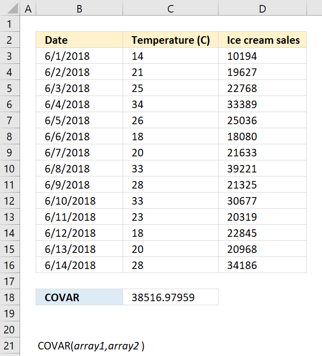
8.3. Example
Formula in cell C18:
8.4. Function not working
Text, logical or empty values are ignored, however, 0 (zeros) are included.
The COVAR function returns
- #N/A error value if the number of data points in array1 and array2 is not equal.
- #DIV/0! error value if either array1 or array2 is empty.
8.5 How is the COVARIANCE.P Function calculated

To calculate the covariance for a population follow these steps:
- Calculate the mean of group of numbers named:
x="Temp"
y="Icecream"
For example:
Mean of X = x̄ is calculated in cell C10
Mean of Y = ȳ is calculated in cell D10 - For each data point xi and yi calculate the deviations from the mean.
Deviation of xi = xi - x̄ are calculated in cells E3:E9
Deviation of yi = yi - ȳ are calculated in cells F3:F9 - Multiply the deviations between each data point pair to get their products.
For each pair: (xi - x̄) * (yi - ȳ) are calculated in cells G3:G9 - Sum all the deviation products.
S = Σ(xi - x̄)(yi - ȳ) calculated in cell G10 - The covariance is the sum of products divided by the number of samples.
The equation for COVARIANCE.P is:

COVARIANCE.P(x,y) = (Σ(xi - x̄)(yi - ȳ))/n
x̄ is the sample means AVERAGE(array1)
ȳ is the sample means AVERAGE(array2)
n is the sample size.
9. How to use the CRITBINOM function

How to use the CRITBINOM function?
The CRITBINOM function calculates the minimum value for which the binomial distribution is equal to or greater than a given threshold value.
The CRITBINOM function is outdated and has been replaced with the BINOM.INV function, although it still exists for compatibility with earlier Excel versions. The CRITBINOM function is located in the compatibility category and may be removed in a future Excel version.
What is the binomial distribution probability?
The binomial distribution probability gives the likelihood of a specific number of successes occurring in a fixed number of independent trials, each having the same binary success/failure probability.
What is an independent trial in terms of binomial distribution?
An independent trial in the context of the binomial distribution refers to each individual test or instance having two possible outcomes, success or failure, in which the result of one trial does not affect the probability of success in subsequent trials.
What is a binary success/failure probability?
A binary success/failure probability describes two mutually exclusive possible outcomes of a trial, conventionally labeled as "success" with probability p and "failure" with probability 1-p, that sum to 1, like heads or tails on a coin flip.
What is binomial?
The binomial is a discrete probability distribution that models the number of successes in a fixed number of independent trials, each with a binary success/failure outcome and a constant success probability across trials.
What is a distribution in statistics?
A distribution in statistics refers to a function representing the frequencies of different potential outcomes for a random variable or dataset, summarized visually in a histogram or mathematically with a probability distribution function.
What is cumulative binomial distribution?
The cumulative binomial distribution function gives the probability that a binomial random variable with a given number of trials and success probability will take on a value less than or equal to a specified number of successes x.
What is the inverse cumulative binomial distribution?
The binomial cumulative distribution calculates the probability of having X or fewer successes in N trials with probability P. The inverse cumulative binomial distribution does the reverse - it finds the number of successes X given a certain cumulative probability.
What is the difference between the binomial distribution and the normal distribution?
The binomial distribution models discrete counts in a fixed number of binary trials, while the normal distribution models continuous real-valued outcomes with symmetry around the mean. As n increases, binomial approaches normal distribution.
What is discrete?
Data that can take on only specific, countable values. For example, number of items.
What is continuous?
Data that can take on any value within a range. For example, temperature, weight, time.
What is the difference between the BINOM.INV function and the CRITBINOM function?
Both the BINOM.INV and the CRITBINOM function share the same arguments: number of trials, probability of success/failure, and criterion value.
CRITBINOM(trials,probability_s,alpha)
BINOM.INV(trials,probability_s,alpha)
They seem to use the same math formula to calculate the value because they return the same calculated value if the arguments are the same, however, don't use the CRITBINOM function who knows when Microsoft decides to remove the function.
9.1. Syntax
CRITBINOM(trials,probability_s,alpha)
9.2. Arguments
| trials | Required. How many Bernoulli trials. |
| probability_s | Required. The probability of success in each test. |
| Alpha | Required. The threshold value. |
What are Bernoulli trials?
Bernoulli trials refer to a series of independent experiments or trials that have a binary outcome - success or failure. Each trial can result in just 2 possible outcomes (e.g. heads/tails, pass/fail).
The trials are independent - the outcome of one does not affect the outcome of another. Each trial has the same probability of success, usually denoted by p.
The number of successes in a series of Bernoulli trials follows a binomial distribution. Examples include coin flips, rolls of a die, sampling with replacement.
Bernoulli trial assumptions are needed for the binomial probability distribution to apply. The name comes from Swiss mathematician Jakob Bernoulli. They are useful for modeling phenomena in statistics, economics, computer science and other fields.
9.3. Example 1
The probability that a customer accepts an offer is estimated to be 70%. The offer is given to 30 customers. How many of them accepts the offer if alpha (probability value) is 0.5?
The inverse binomial distribution is what we need to calculate the number of customers that accepts the offer. It calculates the minimum value for which the cumulative binomial distribution is equal to or greater than a given threshold value which is 0.5 (50%) in this example shown in cell C16 in the image above.
The number of trials is the total number of customers, cell C17 contains 30 meaning there are 30 customers.
In other words, alpha is the probability value for which you want to find the smallest value of x. Each trial has the same probability of success (0.7 or 70%) meaning 70% is the probability a customer accepts the offer. The probability value i specified in cell C18 displayed in cell C18 in the image above.
Formula in cell C8:
The formula returns 21. This means that the smallest number of customers who accept the offer (x) for which the cumulative probability of getting x or fewer customers accepting the offer is greater than or equal to 0.5 (or 50%) is 21. If the probability value (alpha) is 0.5, at least 21 out of the 30 customers will accept the offer.
We can check the value 21 using the BINOM.DIST function and calculate the probability (alpha) value.
The BINOM.DIST function above returns approx. 0.568 (56.8%) for 21 customers. 20 customers returns 0.411 (41.1%) 21 customers satisfies the alpha condition equal to 0.5 (50%) or larger.
The chart in the image above shows an orange line representing the cumulative probability. Go to 0.7 on the secondary y-axis to the right and find the value of x that intersects. The x-axis shows 21 which seems to match the calculated number 21.
9.4 Example 2

There are 15 machines that operate independently of each other in a factory. The probability of a breakdown occurring during a day is 0.2 for each of the machines. How many machines will stop during a certain day if alpha is 0.8 (probability)?
The inverse binomial distribution lets you calculate the number of machines that breaks down based on a independent probability of 0.2 (20%), a total of 15 machines (trials) and alpha (probability) is 0.8 or 80%.
The probability_s argument is specified in cell C18, trials argument is given in cell C17, and the alpha argument is in cell C16.
The formula returns 4. This means that the smallest number of machines that break down during a certain day for which the cumulative probability is greater than or equal to 0.8 (or 80%) is 4.
We can check the value 4 using the BINOM.DIST function and calculate the probability (alpha) value.
The BINOM.DIST function above returns approx. 0.836 (83.6%) for 4 machines. 3 machines return 0.648 (64.8%). 4 machines satisfies the alpha condition equal to 0.8 (80%) or larger.
9.5. Example 3

There are 25 students in a class. There is a 40% risk that each student, independently of each other, will catch a harmless but highly contagious cold. How many will attend school on the same day if the alpha is 0.95 (95%)?
Arguments
- trials : total number of students in the class: 25 (cell C17)
- probability_s : Probability of catching the cold for each student (probability of success): 0.4 or 40% (cell C18)
- alpha : The probability value (α) is 0.95 or 95% (cell C16)
We want to find the smallest value of x (the number of students who will not catch the cold) for which the cumulative binomial probability is greater than or equal to 0.95.
Formula in cell C21:
CRITBINOM(25,0.4,0.95) returns 14 students that will catch the cold. 25 -14 equals 11 students who will not catch the cold.
The image above shows a chart, 0.95 on the secondary y-axis (to the right) matches value 14 on the x-axis.
9.6. Function not working
The CRITBINOM function returns a
- #VALUE! error value if any argument is non-numeric.
- #NUM! error value if:
- trials < 0 (zero)
- probability_s < 0 (zero)
- alpha < 0 (zero)
- alpha > 1
10. How to use the EXPONDIST function
What is the EXPONDIST function?
The EXPONDIST function calculates the exponential distribution representing an outcome in the form of probability.
This function is in the compatibility category and has been replaced by the EXPON.DIST function which was introduced in Excel 2010.
What is an exponential distribution?
The exponential distribution is a continuous probability distribution that models the time between events in a Poisson point process. It is characterized by a constant hazard rate so that the conditional probability of an event does not depend on how much time has passed already.
What is a hazard rate?
The hazard rate is the conditional probability that an event will occur in a small interval given it has not yet occurred. It is often assumed constant in Poisson processes and given by the exponential distribution's parameter.
What is a Poisson point process?
A Poisson point process is a random collection of points representing events in time or space that follow a Poisson distribution. It has independence between points and a constant rate of average occurrence over any interval.
What is a Poisson distribution?
The Poisson distribution is a discrete probability distribution that models the number of events occurring in a fixed interval of time or space. The events must be independent and their average rate is known and constant.
What is independence between points?
Independence between points means that the position or timing of one point in a stochastic spatial or temporal point process does not affect or influence the probability distribution governing the other points. In other words, it is completely random.
What is a stochastic spatial process?
A stochastic spatial process is a random mechanism for generating points distributed in space according to some probability distribution and spatial relationship between the points.
What is a temporal point process?
A temporal point process generates random events in time such as the arrival of customers or radioactive decay with certain probabilistic properties concerning the timing and intervals between events.
What is memorylessness?
Memorylessness is the property of certain probability distributions like the exponential and geometric where past outcomes do not affect future ones, so the conditional probability stays constant regardless of history.
What is a probability distribution?
A probability distribution lets you analyze how likely different random values occurs, in other words, it shows how often we would expect to see different potential values.
What is a continuous probability distribution?
A continuous probability distribution is defined over an interval and range of continuous values, giving the probability an outcome is exactly equal to any value, and having an area under its probability density curve equal to 1.
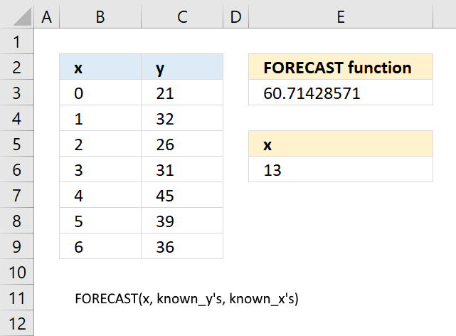
10.1. Syntax
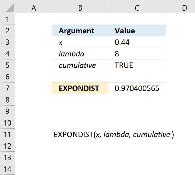
EXPONDIST(x,lambda,cumulative)
10.2. Arguments
| x | Required. |
| lambda | Required. |
| cumulative | Required. A boolean value. TRUE - cumulative distribution function FALSE - probability density function |
10.3. Example
Formula in cell C7:
10.4. Function not working
The EXPONDIST function returns
- #VALUE! error value if lambda or x is non-numeric.
- #NUM! error value if:
- x < 0 (zero)
- lambda <= 0 (zero)
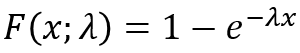
10.5. How is the EXPONDIST Function calculated?
The general equation to calculate the cumulative distribution function:
The general equation to calculate the probability density distribution:
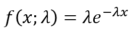
11. How to use the FDIST function
What is the FDIST function?
The FDIST function calculates the F probability of the right-tailed distribution for two tests. The F.DIST function lets you find out if the means between two given populations are significantly different.
What is the F probability?
The F-distribution or F-ratio is a continuous probability distribution that compare the variances of two populations.
What is variance?
The variance shows how much a set of numbers are spread out from their average value.
Σ(x- x̄)2/(n-1)
x̄ is the sample mean
n is the sample size.
What is a null distribution?
The null hypothesis in the F-distribution is that two independent normal variances are equal. If the observed ratio is too large or too small, then the null hypothesis is rejected, and we conclude that the variances are not equal.
When is a f-distribution used?
The F-distribution is used in the F-test in analysis of variance comparing two variances, as the distribution of the ratio of sample variances when the null is true of no difference between population variances.
What is a continuous probability distribution?
A continuous probability distribution is defined over an interval and range of continuous values, giving the probability an outcome is exactly equal to any value, and having an area under its probability density curve equal to 1.
What are the differences between the F.DIST function and the F.DIST.RT function?
The F.DIST function gives the left-tail area under the curve, while the F.DIST.RT function gives the right-tail area under the curve.
The F.DIST function calculates the cumulative distribution function for the F-distribution, which means it returns the probability that a random variable with an F-distribution is less than or equal to the input F-value.
The F.DIST.RT function calculates the right-tailed probability of the F-distribution, which means it returns the probability that a random variable with an F-distribution is greater than the input F-value.
F.DIST.RT(x, deg_freedom1, deg_freedom2)
F.DIST(x, deg_freedom1, deg_freedom2, cumulative)
11.1 Syntax
FDIST(x, deg_freedom1, deg_freedom2)
11.2 Arguments
| x | Required. |
| deg_freedom1 | Required. Degrees of freedom (numerator). |
| deg_freedom2 | Required. Degrees of freedom (denominator). |
What are the degrees of freedom?
The degrees of freedom parameters are the numerator and denominator chi-squared distributions. They form the ratio that follows the F-distribution.
The degrees of freedom parameters affect the shape of the F-distribution curve and probability, they relate to the samples and capture the amount of information in the variance estimates.
What is a chi-squared distribution?
A chi-squared distribution is a type of probability distribution that is used in statistical tests that compare the variances of two populations. The chi-squared distribution has one parameter, called degrees of freedom, that determines its shape and location. The degrees of freedom represent the number of independent pieces of information used to estimate the variances.
11.3. Example
Formula in cell C7:
11.4. Function not working
The FDIST function returns
- #VALUE! error value if any argument is non-numeric.
- #NUM! error value if:
- x < 0 (zero)
- deg_freedom1 < 1
- deg_freedom1 >= 10^10
- deg_freedom2 < 1
- deg_freedom1 >= 10^10
deg_freedom1 and deg_freedom2 will be converted into integers if they are not.
12. How to use the FLOOR function
What is the FLOOR function?
The FLOOR function rounds a number down, toward zero, to the nearest multiple of significance.
The function has been replaced by the FLOOR.PRECISE and FLOOR.MATH functions, although it still exists for compatibility with earlier Excel versions.
The FLOOR function may be removed in a future Excel version, use only for backwards compatibility in older software and workbooks.
What is rounding a number?
Rounding is a method to simplify a number by reducing its digits while keeping its approximate value close to the original value.
There are a few common ways to round:
- Round to a set number of decimal places, rounding 2.13579 to 2 decimal places gives 2.14.
- Round up or down to the nearest integer, rounding up 2.3 gives 3. Rounding down 2.3 gives 2.
- Round to a set increment, rounding to the nearest 10 rounds 17 to 20.
- Round to significant figures, rounding 2.333 to 3 significant figures gives 2.33.
When rounding, look at the first digit after where you want to round. If it's 5 or more, round up. If less than 5, round down. Rounding makes numbers cleaner and easier to work with in many everyday situations, however, they may also cause rounding errors like rounded values can compound errors. Rounding measurements and constants may reduces precision. It is better to round numbers after performing calculations than before.
What is a decimal place?
A decimal place refers to each position held by a digit in a number. The first decimal place is the tenths place (1/10), the second is the hundreds place (1/100) and so on.
What is the nearest multiple of significance?
The nearest multiple of significance means to the closest number that a value gets rounded to for a given level of precision. It is based on the number of significant figures or decimal places desired.
For a certain precision, it is the nearest multiple of a power of 10.
For 2 significant figs, nearest multiples are 10, 100, 1000, etc.
For 3 decimal places, nearest multiples are 0.001, 0.01, 0.1, 1, 10, etc.
Values get rounded to the closest multiple of significance at the desired precision. So if reporting to 2 significant figures, 4874 would round to 4900, since the nearest multiple of significance is 100 at that precision.
If reporting to 3 decimal places, 15.4732 would round to 15.473, since the nearest multiple is 0.001. This helps keep rounding consistent and at an appropriate level of precision when doing math calculations and measurements.
What is an integer?
An integer is a whole number that can be positive, negative, or zero, but not a fraction or decimal.
What other Excel functions round numbers?
| ROUND | Rounds a number to a specified number of digits |
| ROUNDUP | Rounds a number up, away from zero |
| ROUNDDOWN | Rounds a number down, towards zero |
| MROUND | Rounds a number to the nearest multiple of a specified value |
| CEILING | Rounds a number up to its nearest multiple. |
| ODD | Returns number rounded up to the nearest odd integer. |
| EVEN | Rounds a number up to the nearest even whole number. |
| FIXED | Rounds a number to the specified number of decimals, lets you ignore comma separators. |
| FLOOR.PRECISE | Rounds a number down to the nearest integer or nearest multiple of significance. |
| FLOOR.MATH | Rounds a number down to the nearest integer or to the nearest multiple of significance. |
12.1. Syntax
FLOOR(number, significance)
12.2. Arguments
| number | Required. The number you want to round. |
| significance | Required. The multiple to which you want to round. |
- A value is rounded down and adjusted toward zero if the number argument is positive.
- A value is rounded down and adjusted away from zero if the number argument is negative.
- No rounding occurs if number is an exact multiple of significance.
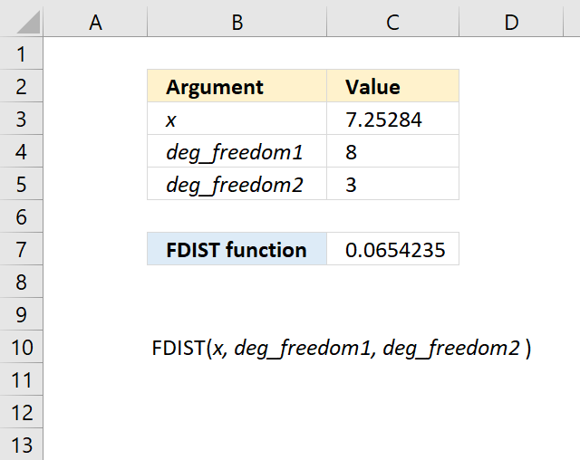
12.3. Example
This example demonstrates how to round numbers using the FLOOR function. The first example shown in row three takes number 3.7 and calculates the nearest multiple of significance based argument significance which is specified to 2. The result is 2.
Formula in cell C3:
The second example uses a negative input value in the first argument number which is -2.5 and the significance argument which is specified to -2. The formula in cell C4 returns -2 which is the nearest multiple of significance of -2.
12.4. Function not working
The FLOOR function returns:
- the #VALUE! error value if either argument is nonnumeric.
- the #NUM! error value if number is positive and significance is negative.
13. How to use the FORECAST function
What is the FORECAST function?
The FORECAST function calculates a value based on existing x and y values using linear regression. Use this function to predict linear trends.
There are newer better functions that may have improved accuracy, this function is available for compatibility with older workbooks created in earlier Excel versions and other older software.
This function is outdated and was replaced with FORECAST.LINEAR function in Excel 2016. Microsoft informs that the FORECAST function may not be available in future Excel versions and recommends using the FORECAST.LINEAR function from now on.
What is linear regression?
Linear regression is a statistical technique used to model the linear relationship between a dependent variable and one or more independent variables.
It fits a straight line through the set of data points in such a way that the sum of squared residuals (error) between the line and the points is minimized.
The line equation is defined as Y = a + bx.
Where Y is the dependent variable
x is the independent variable
b is the slope of the line
a is the y-intercept
Regression analysis generates the slope, intercept, and ultimately the line equation that models the relationship between the variables.
What is the slope?
The slope (b) represents the change in Y associated with a unit change in x. Excel lets you calculate the slope with the SLOPE function.
What is the intercept?
The y-intercept (a) is where the line crosses the y-axis when x=0. Excel lets you calculate the intercept with the INTERCEPT function.
What is the R-squared?
R-squared (R2) represents how well the line fits the data. The closer to 1, the better the regression line fits the data. The LINEST function lets you calculate the R-squared value based on known y and known x.
Other ways to calculate the linear regression?

Excel lets you add the linear equation and the line if you plot the data on a scatter chart, simply press with left mouse button on the plus button located on the upper right corner next to the chart. You must select the chart to see the plus button.
Press with left mouse button on the arrow next to the trendline and then press with left mouse button on "Linear Forecast". Double press with left mouse button on the dotted line on the chart to see the settings pane. Press with left mouse button on the checkboxes "Display the equation the chart" and the "Display the R-squared value on the chart" to show the linear regression data on the chart.
What is a linear equation?
A linear equation is a type of equation that can be written in the form ax + b = 0, where a and b are constants and x is a variable. A linear equation represents a relationship between two quantities that are proportional to each other.
For example, if you have a linear equation that says y = 3x + 4, it means that for every unit increase in x, the value of y increases by 3 units and when x is zero y is 4.
The graph of a linear equation is always a straight line, a linear equation does not involve powers of variables.
What is the difference between the FORECAST and the FORECAST.LINEAR function?
The FORECAST function is a legacy function available for compatibility with older software.
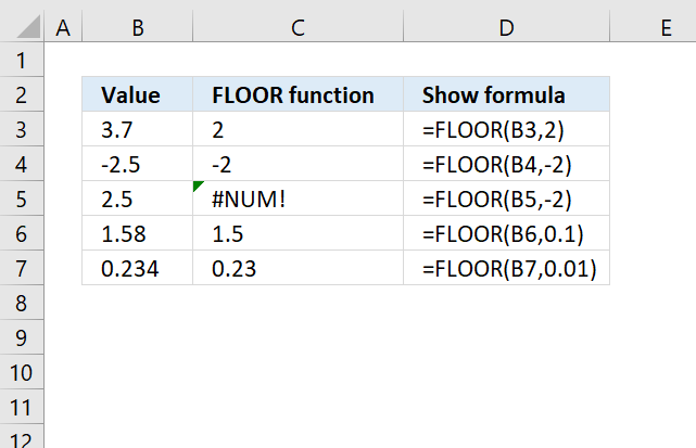
13.1 Syntax
FORECAST(x, known_y's, known_x's)
13.2 Arguments
| x | Required. The data point for which you want to predict a value. |
| known_y's | Required. Known y points. |
| known_x's | Required. Known x points. |
13.3 Example
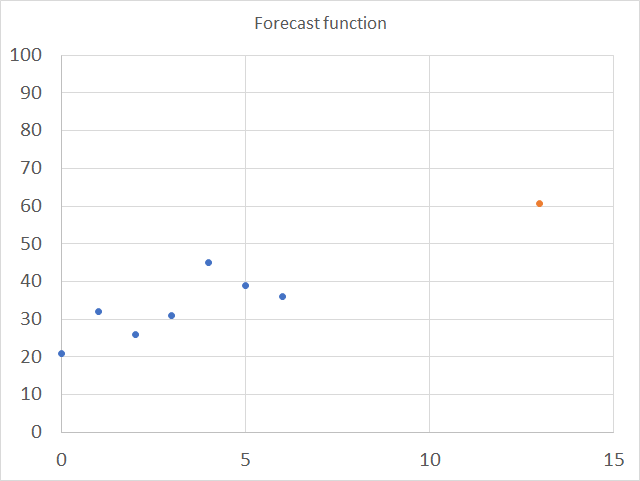
Formula in cell E3:
The chart below shows the predicted value as a red dot, based on x and y values represented by the blue dots.
13.4 Function not working
FORECAST function returns a
- #VALUE error if x is not numeric.
- #N/A error if known_y's or known_x's is left out.
- #DIV/0! error value if the variance of known_x's evaluates to zero.
13.5 What is the formula behind the FORECAST function
The mathematical formula behind calculating a simple linear regression is based on minimizing the sum of squared residuals (errors) between the regression line and data points.
Let (x1, y1), (x2, y2), ..., (xn, yn) be the dataset of n points.
The goal is to find the intercept a and slope b for the line equation:
y = a + bx
That minimizes the sum of squared residuals (SSres):
SSres = Σ(yi - ŷi)2
Where ŷi is the predicted y value for point i based on the line. By taking the derivatives of SSres with respect to a and b, setting them equal to 0, and solving, we get:
a = y̅ - b*x̅
b = Σ(xi - x̅)*(yi - y̅) / Σ(xi - x̅)2
Where x̅ and y̅ are the mean values.
This gives the least squares regression line that best fits the data by minimizing the residual sum of squares.
14. How to use the FTEST function
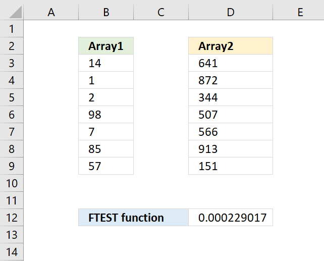
What is the FTEST function?
The FTEST function calculates the value from an F-test. The value shows if the variances from two data sets are not significantly different.
What is the two-tailed probability from an F-test?
The two-tailed probability from an F-test refers to testing against the alternative hypothesis that the two population variances are not equal without specifying direction.
The F-test compares two sample variances by forming a ratio that follows an F-distribution. It tests the null hypothesis that the population variances are equal.
If the variances are not equal which can occur in either direction meaning one could be larger or smaller. A two-tailed test checks both flanks of the F distribution for the probability that the ratio is quite large or quite small. The two-tailed p-value is the total area in both tails combined.
What is a hypothesis in statistics?
In statistics, a hypothesis is an assumption about some aspect of a population or underlying probability model. Hypotheses are of two main types:
- Null hypothesis (H0) - Represents the status quo. Asserts there is no meaningful effect, relationship, or difference in the parameter of interest between groups.
- Alternative hypothesis (H1) - Asserts there is a statistically significant effect in the parameter. Reflects a potential research finding or relationship.
A statistical hypotheses state an assumption that can be tested to reach conclusions from experimental data using methods like t-tests, ANOVA, or chi-square tests.
What is the F probability?
The F-distribution or F-ratio is a continuous probability distribution that compare the variances of two populations.
What is variance?
The variance shows how much a set of numbers are spread out from their average value.
Σ(x- x̄)2/(n-1)
x̄ is the sample mean
n is the sample size.
What is a null distribution?
The null hypothesis in the F-distribution is that two independent normal variances are equal. If the observed ratio is too large or too small, then the null hypothesis is rejected, and we conclude that the variances are not equal.
When is a f-distribution used?
The F-distribution is used in the F-test in analysis of variance comparing two variances, as the distribution of the ratio of sample variances when the null is true of no difference between population variances.
What is a continuous probability distribution?
A continuous probability distribution is defined over an interval and range of continuous values, giving the probability an outcome is exactly equal to any value, and having an area under its probability density curve equal to 1.
14.1 Syntax
FTEST(array1, array2)
14.2 Arguments
| array1 | Required. The first data set. |
| array2 | Required. The second data set. |
14.3 Example
Formula in cell D12:
14.4 Function not working
The arguments must contain numbers or cell references to numbers.
Text, boolean and empty values are ignored.
The FTEST function returns
- #DIV/0! error value if the number of items in each data set don't match.
- #VALUE! error value if any argument is non-numeric.
14.5 How to calculate F statistics?
The LINEST function calculates the F statistic whereas the FTEST function calculates the probability.
14.6 How to calculate the Ftest using an Excel add-in
15. How to use the GAMMADIST function
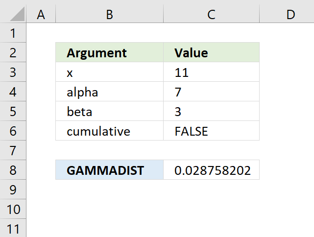
What is the GAMMADIST function?
The GAMMADIST function calculates the gamma often used in queuing analysis in probability statistics.
What is a gamma distribution?
The gamma distribution is a two-parameter continuous probability distribution defined for positive values. It generalizes other distributions like chi-square and exponential and models positively skewed data like time durations.
What is queuing analysis in probability statistics?
Queuing analysis involves using probability and statistics to analyze and model queues (waiting lines). Studies arrival patterns, service times, queue capacity to describe performance and uses probability distributions like Poisson and exponential distributions. It calculates key metrics like expected wait times, queue lengths, utilization.
What is a skewed distribution?
Skewness and asymmetric tails describe the lack of balance and symmetry in probability distributions and datasets. Identifying skewness is fundamental in statistics.
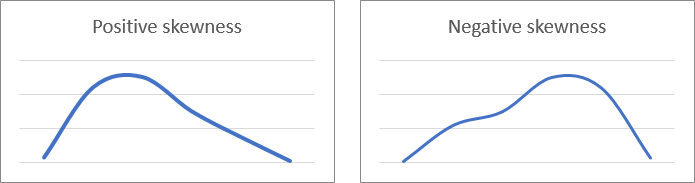
Positive skewness implies a group of values with an asymmetric tail moving toward more positive values. Negative skewness implies a group of values with an asymmetric tail moving toward more negative values.
What is an asymmetric tail?
A symmetric distribution like the normal distribution has no skewness. An asymmetric tail is when one tail of the distribution extends further than the other.
15.1 Example
Formula in cell C7:
15.2 Syntax
GAMMADIST(x,alpha,beta,cumulative)
15.3 Arguments
| x | Required. |
| alpha | Required. |
| beta | Required. 1 returns the standard gamma distribution. |
| cumulative | Required. A boolean value. TRUE - cumulative distribution function FALSE - probability density function |
What is a density function?
A density function in statistics describes the relative likelihood that a random variable takes on a given value. The area under the entire density function integrates to 1.
There are two main types of density functions:
- Probability Density Function (PDF)
PDFs are used for continuous random variables and provides the probability that the variable's value lies within a small range around x.
The area under PDF over an interval provides the probability that the variable lies within that interval. - Probability Mass Function (PMF)
PMFs are used for discrete random variables and gives the exact probability that a variable takes on a specific value x.
15.4 Function not working
The GAMMADIST function returns
- #VALUE! error value if alpha, beta or x is non-numeric.
- #NUM! error value if:
- x < 0 (zero)
- alpha <= 0 (zero)
- beta <= 0 (zero)
15.5 How is the GAMMADIST function calculated?
The equation to calculate the gamma probabiltiy density function:
The standard gamma probability function:
16. How to use the LOGNORMDIST function
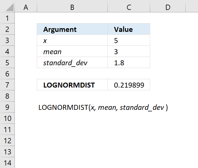
What is the LOGNORMDIST function?
The LOGNORMDIST function calculates the cumulative lognormal distribution of argument x, based on a normally distributed ln(x) with the arguments of mean and standard_dev.
What is the lognormal distribution?
The lognormal distribution is a continuous probability distribution of a random variable whose logarithm follows a normal distribution. It is often used to model a steady relative growth rate is steady like financial returns.
What is a normally distributed ln(x)?
For a random variable x that follows a lognormal distribution like ln(x) is normally distributed. This means that if you take the natural logarithm of x the result will follow a standard normal distribution.
What is a continuous probability distribution?
A continuous probability distribution is defined over an interval and range of continuous values. This gives the probability an outcome that is exactly equal to any value, and having an area under its probability density curve equal to 1.
What is a continuous value?
A continuous value comes from a continuum of possible points rather than distinct separate values. It is able to take on any quantity within an interval rather than certain fixed outcomes.
16.1 Example
Formula in cell C7:
16.2 Syntax
LOGNORMDIST(x, mean, standard_dev)
16.3 Arguments
| x | Required. |
| mean | Required. A value representing the mean of ln(x). |
| standard_dev | Required. A value representing the standard deviation of ln(x). |
What is the mean?
The arithmetic mean is calculated by dividing the sum of all values by the number of values.
For example, an array contains these values: 3,2,1
The sum is 3 + 2 + 1 equals 6
The number of values is 3.
6/3 equals 2. The average of 3, 2, 1 is 2
What is the standard deviation?

Standard deviation tells you how far from the average values are spread out. Both charts above have numbers and an average plotted, they share the same average however, the numbers are not the same.
Chart A above shows that the values are more spread out than the values in chart B. Chart A has a standard deviation of 23.45256334, standard deviation for chart B is 5.207075606. Standard deviation is used in statistics.
What is the cumulative distribution function?
The cumulative distribution function defines the probability that a random variable is less than or equal to a specified value. It gives the area under the probability density curve up to that value.
What is the probability density function?
A probability density function defines a continuous probability distribution by providing the relative likelihood that a random variable takes on different values. The total area under the curve over all values equal to 1.
16.4 Function not working
The LOGNORMDIST function returns
- #VALUE! error value if any argument is non-numeric.
- #NUM! error value if:
- x <= 0
- standard_dev <= 0
16.5 How is the LOGNORMDIST Function calculated?
The equation to calculate the lognormal cumulative distribution is:

17. How to use the MODE function
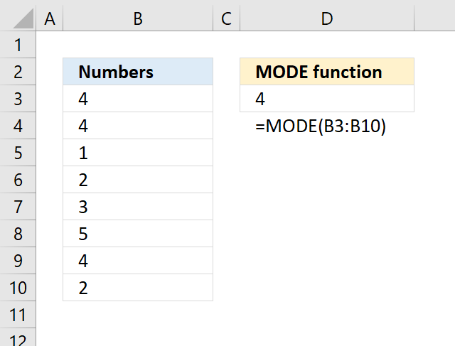
The MODE function calculates the most frequent number in a cell range.
Number 4 exists 3 times on picture above and number 2 exists only 2 times. Number 4 is the most frequent number in B3:B10.
17.1 Syntax
MODE(number1,[number2],...)
17.2 Arguments
| number1 | Required. A cell range you want to calculate the most frequent number. |
| [number2] | Optional. Up to 254 additional arguments. |
17.3 How to get the most common text value

Formula in cell D3:
Explaining formula in cell D3
Step 1 - Create a number representing the position of each value in a sorted array
The COUNTIF function calculates the number of cells equal to a condition. In this case, the less than character compares all values and assigns a number to each value based on their position in a sorted array.
COUNTIF(range, criteria)
COUNTIF(B3:B12, "<"&B3:B12)
becomes
COUNTIF({"Emphasis"; "Basil"; "Boolean"; "Emphasis"; "Gift"; "Historian"; "Boolean"; "Pension"; "Emphasis"; "Yogurt"},"<"&{"Emphasis"; "Basil"; "Boolean"; "Emphasis"; "Gift"; "Historian"; "Boolean"; "Pension"; "Emphasis"; "Yogurt"})
and returns
{3; 0; 1; 3; 6; 7; 1; 8; 3; 9}
Repeated values have identical numbers, we can use this to extract the most common number, see next step.
For example, "Boolean" is displayed twice in B3:B12, shown in the image above. The corresponding number in the array is 1, 1 is shown twice in the array.
Step 2 - Get the most repeated number
The MODE function returns the most common number in a cell range or array.
MODE(COUNTIF(B3:B12, "<"&B3:B12))
becomes
MODE({3; 0; 1; 3; 6; 7; 1; 8; 3; 9})
and returns 3. Number three is the most common number in the array.
Step 3 - Find the position of most repeated number
The MATCH function returns the relative position of an item in an array or cell reference that matches a specified value in a specific order.
MATCH(lookup_value, lookup_array, [match_type])
MATCH(MODE(COUNTIF(B3:B12, "<"&B3:B12)), COUNTIF(B3:B12, "<"&B3:B12), 0)
becomes
MATCH(3, COUNTIF(B3:B12, "<"&B3:B12), 0)
becomes
MATCH(3, {3; 0; 1; 3; 6; 7; 1; 8; 3; 9}, 0)
and returns 1. Three is the first value in the array.
Step 4 - Get value based on position
The INDEX function returns a value from a cell range, you specify which value based on a row and column number.
INDEX(array, [row_num], [column_num], [area_num])
INDEX(B3:B12, MATCH(MODE(COUNTIF(B3:B12, "<"&B3:B12)), COUNTIF(B3:B12, "<"&B3:B12), 0))
becomes
INDEX(B3:B12, 1)
becomes
INDEX({"Emphasis"; "Basil"; "Boolean"; "Emphasis"; "Gift"; "Historian"; "Boolean"; "Pension"; "Emphasis"; "Yogurt"}, 1)
and returns "Emphasis".
17.4 How to get the most common text value - Excel 365
Formula in cell D3:
Explaining formula in cell D3
Step 1 - Count how many times each value is repeated in the array
The COUNTIF function calculates the number of cells equal to a condition.
COUNTIF(range, criteria)
COUNTIF(B3:B12,B3:B12)
becomes
COUNTIF({"Emphasis"; "Basil"; "Boolean"; "Emphasis"; "Gift"; "Historian"; "Boolean"; "Pension"; "Emphasis"; "Yogurt"}, {"Emphasis"; "Basil"; "Boolean"; "Emphasis"; "Gift"; "Historian"; "Boolean"; "Pension"; "Emphasis"; "Yogurt"})
and returns {3; 1; 2; 3; 1; 1; 2; 1; 3; 1}.
Step 2 - Find the largest value
The MAX function returns the largest number in a cell range or array.
MAX(COUNTIF(B3:B12,B3:B12))
becomes
MAX({3; 1; 2; 3; 1; 1; 2; 1; 3; 1})
and returns 3.
Step 3 - Calculate the position of the largest value in array
The equal sign lets you compare value to value, it returns boolean values TRUE or FALSE.
MAX(COUNTIF(B3:B12,B3:B12))=COUNTIF(B3:B12,B3:B12)
becomes
3=COUNTIF(B3:B12, B3:B12)
becomes
3={3; 1; 2; 3; 1; 1; 2; 1; 3; 1}
and returns {TRUE; FALSE; FALSE; TRUE; FALSE; FALSE; FALSE; FALSE; TRUE; FALSE}.
Step 4 - Filter corresponding value
The FILTER function extract values/rows based on a condition or criteria.
FILTER(array, include, [if_empty])
FILTER(B3:B12, MAX(COUNTIF(B3:B12,B3:B12))=COUNTIF(B3:B12,B3:B12))
becomes
FILTER(B3:B12, {TRUE; FALSE; FALSE; TRUE; FALSE; FALSE; FALSE; FALSE; TRUE; FALSE})
becomes
FILTER({"Emphasis"; "Basil"; "Boolean"; "Emphasis"; "Gift"; "Historian"; "Boolean"; "Pension"; "Emphasis"; "Yogurt"}, {TRUE; FALSE; FALSE; TRUE; FALSE; FALSE; FALSE; FALSE; TRUE; FALSE})
and returns {"Emphasis"; "Emphasis"; "Emphasis"}.
Step 5 - Extract unique distinct values
The UNIQUE function extracts both unique and unique distinct values and also compares columns to columns or rows to rows.
UNIQUE(array, [by_col], [exactly_once])
UNIQUE(FILTER(B3:B12, MAX(COUNTIF(B3:B12,B3:B12))=COUNTIF(B3:B12,B3:B12)))
becomes
UNIQUE({"Emphasis"; "Emphasis"; "Emphasis"})
and returns "Emphasis".
Step 6 - Shorten formula
The LET function lets you name intermediate calculation results which can shorten formulas considerably and improve performance.
LET(name1, name_value1, calculation_or_name2, [name_value2, calculation_or_name3...])
The following formula can be shortened using the LET function, cell range B3:B12 is repeated many times in the formula.
Function COUNTIF(B3:B12,B3:B12) is also repeated in the formula, I have assigned z to B3:B12 and y to COUNTIF(B3:B12, B3:B12).
UNIQUE(FILTER(B3:B12, MAX(COUNTIF(B3:B12,B3:B12))=COUNTIF(B3:B12,B3:B12)))
becomes
LET(z, B3:B12, y, COUNTIF(z, z), UNIQUE(FILTER(z, MAX(y)=y)))
18. How to use the PERCENTRANK function
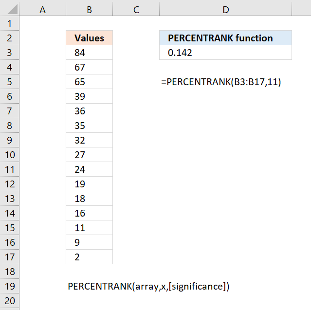
The PERCENTRANK function calculates the percent rank of a given number compared to the whole data set.
What is the percent rank?
The percent rank (or percentile rank) indicates the percentage of scores that fall at or below a given score in a dataset. It provides a way to evaluate the standing of a score relative to others.
What is relative standing?
Relative standing refers to how a particular score compares to the distribution of scores within a group or population. It allows you to understand where a score ranks in relation to others.
When is the PERCENTRANK function useful?
Use the PERCENTRANK.EXC function to evaluate the standing of an aptitude test score among all scores for the test.
What is an aptitude test score?
An aptitude test is a standardized test designed to measure a person's ability or skills in a specific topic. An aptitude test score is the performance measurement on such a test.
Evaluating an aptitude test score's percentage ranking allows understanding its standing compared to other test takers. Higher percentiles indicate better relative performance on the aptitude test.
18.1 Syntax
PERCENTRANK(array, x, [significance])
18.2 Arguments
| array | Required. The array or range of data with numeric values that defines relative standing. |
| x | Required. The value for which you want to know the percent rank. |
| [significance] | Optional. Lower bound, default value 0 (zero). |
What are significant digits?
The PERCENTRANK function does not round the output number to the specified number of significant digits. If the specified number is 3 then 0.1875 becomes 0.187 which means that the remaining digits are simply removed.
18.3 Example
The image above shows 15 numbers in column B. The formula calculates the percent rank for number 11.
Formula in cell C7:
2 numbers are less than 11 (second argument) and 12 numbers are larger than 11.
2/(2+12) = 0.142 (approx 3 digits)
What is percent?
A percent represents a fraction or ratio with a denominator of 100. The term comes from "per cent" meaning out of 100.
A percent expresses a number as a fraction of 100. Converting a fraction or decimal to a percentage involves multiplying by 100 and adding a % symbol. For example, 30% means 30/100 or 0.3. A percentage represents the relative proportion of some quantity compared to 100 units of that quantity
Percentages range between 0% to 100%. 0% means none while 100% means the total amount. They allow standardized measurement of ratios and comparison of part-to-whole relationships. Used frequently in statistics, business, banking, science and other areas involving relative amounts.
What if the x value is not in the array?
The PERCENTRANK function interpolates in order to return the correct value if x doesn't match a value in the array.
What is interpolate?
Interpolate means to estimate or infer a data point within a range of known data points. In statistics, interpolation refers to estimating the percentage between existing data points in a distribution.
18.4 Function not working
The PERCENTRANK function returns
- #NUM! error value if:
- array is empty
- [significance] < 1
19. How to use the QUARTILE function
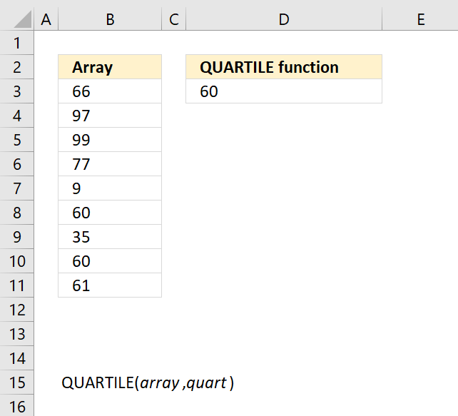
What is the QUARTILE function?
The QUARTILE function returns the quartile of a data set, use the QUARTILE function to divide data into groups.
What is a quartile?
A quartile is a type of quantile which splits a dataset into four equal parts. The quartiles divide a rank-ordered dataset into four quarters.
There are three quartile values - Q1, Q2, and Q3:
Q1 (first quartile) - 25th percentile
Q2 (second quartile) - 50th percentile (median)
Q3 (third quartile) - 75th percentile
What is the interquartile range (IQR)?
The interquartile range (IQR) is the difference between Q3 and Q1. It indicates the middle 50% spread of the data.
When is it useful to calculate the quartiles?
Quartiles provide quantile-based partitioning of data that reveals distribution, spread, skewness, and outliers. They serve as an important basic statistical summary.
What is quantile?
Quantiles are a statistical technique for dividing a dataset into equal-sized groups for analysis. Quantiles split data into equal-sized subsets when ordered from smallest to largest.
The quartiles, percentiles, quintiles, deciles, etc. are examples of quantiles.
- Quartiles split data into 4 equal groups
- Percentiles into 100 groups,
- Quintiles into 5.
Quantiles can show aspects of shape, spread, and concentration.
How to graph quartiles?
The Box and Whisker chart display quartiles.
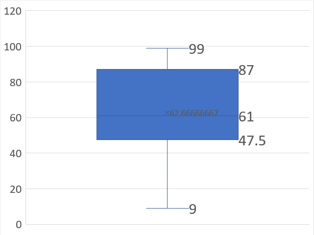
19.1 Syntax
QUARTILE(array, quart)
19.2 Arguments
| array | Required.The cell values for which you want to calculate the quartile value. |
| quart | Required. Indicates which value to return, see table below. |
| Quart parameters | |
|---|---|
| 0 | Minimum value. |
| 1 | First quartile (25th percentile). |
| 2 | Median quartile (50th percentile). |
| 3 | Third quartile (75th percentile). |
| 4 | Maximum value. |
19.3 Example
This example demonstrates the QUARTILE function, the image above shows the following values in B3:B11: 66, 97, 99, 77, 9, 60, 35, 60, 61
Formula in cell D3:
Here is how the QUARTILE function calculates the first Quartile (Q1). The median is 61 based on the numbers in cell range B3:B11. The first half contains the following numbers: 9, 35, 61, 60, and 60 The median of these numbers is 60.
The QUARTILE function returns the same value as:
- MIN function if quart is 0 (zero)
- MEDIAN function if quart is 2.
- MAX function if quart is 4
What is the MEDIAN?
The median value is the middle number of a group of numbers when arranged from smallest to largest. It returns a good measure of the typical value in a data set that is not affected by outliers or skewness . For example, the median income may be a better measure of the average income than the mean. The mean can be distorted by a few very high incomes which is the case, for instance, in the US. The very high incomes represent the outliers.
For example, a group containing an odd number of values like five numbers: 1, 3,4,9, and 11 has the middle value 4. 1 and 3 are smaller and 9 and 11 are larger.
A group containing an even number of values like: 1,3,9, and 11 has a median of 6. There are two middle numbers in the group which are 3 and 9. 3 + 9 = 12 and 12/2 equals 6.
What is the MIN function?
The MIN function returns the smallest number in a cell range.
Function syntax: MIN(number1, [number2], ...)
What is the MEDIAN function?
The MEDIAN function calculates the median based on a group of numbers. The median is the middle number of a group of numbers.
Function syntax: MEDIAN(number1, [number2], ...)
What is the MAX function?
The MAX function calculate the largest number in a cell range.
Function syntax: MAX(number1, [number2], ...)
19.4 Function not working
The QUARTILE function returns #NUM! value if
- quart < 0 (zero)
- quart > 4
19.5 How is the QUARTILE function calculated?
QUARTILE function calculates quartiles using the inclusive method:
Data is sorted lowest to highest. The quartile boundaries include the quartile values themselves.
For example, for the data {1, 2, 3, 4, 5}:
Q0 = 1
Q1 = 2
Q2 = 3
Q3 = 4
The median of data {1, 2, 3, 4, 5} is 3. The first half contains 1 , 2, and 3. The median of 1,2, and 3 is 2 = Q1
Q2 is the median: 3
The second half contains 3, 4 and 5, The median of 3, 4 and 5 is 4 = Q3
20. How to use the RANK function
![]()
What is the RANK function?
The RANK function calculates the size of a specific number compared to a list of numbers. It allows you to rank numbers relative to their sizes in ascending or descending order.
There are newer better functions that may have improved accuracy, this function is available for compatibility with Excel 2007 and earlier versions.
This function is outdated and was replaced with RANK.AVG function and the RANK.EQ function. The RANK function may not be available in future Excel versions and Microsoft recommends using the newer functions from now on.
What are the differences between the RANK, RANK.EQ and RANK.AVG functions?
First, the RANK function is a legacy function and should be avoided if possible. The RANK.EQ function and the RANK function rank numbers based on size, however, they share the rank if two or more numbers are equal. For example:
| Numbers | RANK.EQ | RANK |
| 10 | 4 | 4 |
| 20 | 2 | 2 |
| 20 | 2 | 2 |
| 30 | 1 | 1 |
The RANK.AVG function returns the rank of a number in a list of numbers. If more than one value share the same rank, the average rank is returned. For example:
| Numbers | RANK.AVG |
| 10 | 4 |
| 20 | 2.5 |
| 20 | 2.5 |
| 30 | 1 |
What are the differences between the RANK and PERCENTRANK functions?
The PERCENTRANK function calculates the percent rank of a given number compared to the whole data set.
| Numbers | RANK | PERCENTRANK |
| 10 | 4 | 0 |
| 20 | 2.5 | 0.333 |
| 20 | 2.5 | 0.333 |
| 30 | 1 | 1 |
The PERCENTRANK function is also a legacy function and should be avoided if possible. Use the PERCENTRANK.EXC or the PERCENTRANK.INC.
Other ways to rank numbers in a list?
![]()
Data Bars is a conditional formatting feature that allows you to create horizontal bars that represent a corresponding number. This allows you to more quickly scan a group of numbers for the largest and smallest numbers.
![]()
Color scales is also a conditional formatting feature that allows you to highlight cells based on the size of their numbers.
Why is ranking numbers useful in statistics?
Ranking numbers in statistics refers to converting data values into their ranked order.
- Reduces the impact of outliers
Extreme values don't distort ranks as much as raw scores. - Easier to interpret
Ranks provide a sense of relative standing on a consistent scale from lowest to highest. - Allows non-parametric tests
Statistical tests that don't rely on parameterized distributions. - Simplifies combining scores
Ranks provide a common scale for scores from different sources. - Assesses relative performance
Ranks indicate how a value compares to others in the dataset. - Analyze changes in rank
Shifts in ranks over time can be meaningful even if values don't change much. - Identify top/bottom performers
Ranks make it easy to find top and bottom values. - Tied ranks for equal values
Accounts for duplicate values getting the same mean rank.
20.1 Syntax
RANK(number,ref,[order])
20.2 Arguments
| number | Required. The number you want to calculate the rank for. |
| Ref | Required. An array or cell reference to a list of numerical values. |
| Order | Optional. How to rank the number, 1 - ascending or 0 - descending. If omitted - descending order. |
What is ascending?
Ascending is a term used to describe the order and sequence of data. Ascending order sorts data from lowest to highest.
Arranging data points from lowest to highest value. Also known as increasing order. The ranking goes up, with smaller values first.
Example: Sorting numbers 1, 2, 3 in ascending order.
What is descending?
Descending is a term used to describe the order and sequence of data. Descending order sorts data from highest to lowest.
Arranging data points from highest to lowest value, also known as decreasing order. The ranking goes down, with larger values first.
Example: Sorting numbers 3, 2, 1 in descending order.
20.3 example
![]()
The image above shows 5 digit numbers in cell range B3:B15, the corresponding cells on the same row in column C shows the rank output from the RANK function. The RANK function returns a number representing the position if they were sorted in ascending or descending order.
Formula in cell C3:
The largest number is in cell B15, cell C15 contains the output from the RANK function which is 1. The smallest number is in cell B12, cell C12 shows 13 which is the rank. There are 13 numbers in cell range B3:B15 and the rank 13 tells us that the number is the smallest based on it's size compared to the other numbers in the list.
![]()
20.4 Alternative
![]()
The COUNTIF function allows you to count cells based on a condition. The smaller than or larger than character lets you count numbers that are smaller or larger respectively.
Formula in cell C3:
The COUNTIF function calculates the number of cells that is equal to a condition.
Function syntax: COUNTIF(range, criteria)
For example, cell range B3:B15 contains five numbers larger than the number in cell C3. The COUNTIF function returns five indicating that the number in cell B3 is the sixth largest number, the reason why is because the COUNTIF function returns 0 (zero) for the largest number in the group. One for the second largest and so on.
To make the COUNTIF function return the same number as the RANK function then add 1 to the function like this:
Why is the COUNTIF function returning 0 (zero) for the largest number in a list?
The COUNTIF function counts the number of cells that contain a number larger than the condition.
For example, there is no number larger than the largest number and that makes the COUNTIF function return 0 (zero).
The COUNTIF function also counts text values, this is demonstrated in the next section below.
20.5 How to rank text
![]()
Did you know that it is possible to rank text strings using the COUNTIF function? It returns a number corresponding to the position in a sorted list except that the top text value starts with 0 (zero).
For example:
A - 0
B - 1
C - 2
D - 3
F - 4
The list above is sorted from A to Z.
Formula in cell C3:
The COUNTIF function is one of the more useful functions in Excel, this is just one example.
Recommended articles

Counts the number of cells that meet a specific condition.
21. How to use the STDEV function

What is the STDEV function?
The STDEV function calculates the standard deviation of a sample of values. The standard deviation shows how much the values differ from the mean value.
There are two different math formulas for calculating the standard deviation, the STDEV function tries estimates the standard deviation based on a sample of values whereas the STDEV.P function calculates the standard deviation based on the entire population.
Section 5 below describes the differences in how the standard deviation is calculated.
There are newer better functions that may have improved accuracy, this function is available for compatibility with older workbooks created in earlier Excel versions and other older software.
The new STDEV.S function replaces the older STDEV function which has better accuracy, Microsoft tells us that the STDEV function may not be available in future Excel versions and recommends us using the STDEV.S from now on.
Table of Contents
21.1. What is Standard Deviation?
Standard deviation tells you how far from the mean values are spread out. Both charts above have numbers and an average plotted, they share the same average however, the numbers are not the same.
Chart A above shows that the values are more spread out than the values in chart B. Standard deviation is used in statistics.
A low standard deviation number near 0 (zero) tells us that the data points are located very close to the mean, a larger standard deviation value indicates data points are more spread out from the mean.
The most commonly used symbol for standard deviation is σ which is the lower case greek letter sigma. σ was chosen because standard deviation is calculated using summation Σ which is the upper case greek letter sigma.
σ is used to represent population standard deviation. s is used to represent sample standard deviation. In statistics formulas, σ is used along with the mean symbol μ to represent a distribution.
What is the mean?
The mean is also called the average. The mean is calculated by adding all the values in a dataset and dividing by the total number of values. Excel has functions for calculating the average. AVERAGE function
For example, a data set contains 5, 2,6,8, and 4. The total is 5 + 2 + 6 + 8 + 4 equals 25. The average is 25 / 5 equals 5.
What is one standard deviation in a normal distribution?

One standard deviation from the mean μ captures 34.13% of the data on each side, or 68.27% total in a standard normal distribution. This percentage allows standard deviations to indicate where values fall in the distribution.
What is two standard deviations in a normal distribution?

Two standard deviations from the mean μ captures 47.5% of the data on each side, or 95% total in a standard normal distribution.
What is three standard deviations in a normal distribution?

Tree standard deviations from the mean μ captures 48.85% of the data on each side, or 97.7% total in a standard normal distribution.
21.2. STDEV Function Syntax
STDEV(number1,[number2],...)
21.3. STDEV Function Arguments
| number1 | Required. This argument can be an array of constants or a cell reference to a group of values. |
| [number2] | Optional. Up to 254 additional arguments. |
21.4. STDEV Function Example
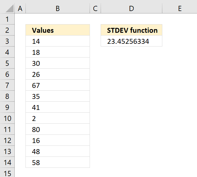
Formula in cell C3:
21.5. How is the STDEV function calculated?
The STDEV function is entered in cell D3, here is how the function calculated the output:

x ̅ is the average.
n is how many values.
Step 1 - Calculate the average
14 + 18 + 30 + 26 + 67 + 35 + 41 + 2 + 80 + 16 + 48 + 58 = 435
435/12 = 36.25
Step 2 - Subtract the average and square the result for all values
(14-36.25)^2 + (18-36.25)^2 + (30-36.25)^2 + (26-36.25)^2 + (67-36.25)^2 + (35-36.25)^2 + (41-36.25)^2 + (2-36.25)^2 + (80-36.25)^2 + (16-36.25)^2 + (48-36.25)^2 + (58-36.25)^2
becomes
(-22.25)^2+(-18.25)^2+(-6.25)^2+(-10.25)^2+(30.75)^2+(-1.25)^2+(4.75)^2+(-34.25)^2+(43.75)^2+(-20.25)^2+(11.75)^2+(21.75)^2
becomes
495.0625+333.0625+39.0625+105.0625+945.5625+1.5625+22.5625+1173.0625+1914.0625+410.0625+138.0625+473.0625
and returns
6050.25
Step 3 - Divide with the total count minus 1
6050.25/11 equals 550.022727272727
Step 4 - Square root the result
550.022727272727^(1/2) equals 23.4525633411942
21.6. What is the difference between the STDEV function and the STEDV.P function?
The STDEV function estimates an output based on a sample of values, the STEDV.P however, calculates the standard deviation based on the entire population of values.
STDEV function formula:
STDEV.P function formula:

These formula differences explain why the functions return different values even if you use the same values.
21.7. What is the difference between the standard deviation and variance?
Standard deviation measures the amount of dispersion around the mean, while variance represents the average squared deviation. Standard deviation provides an interpretable and tangible idea of spread, while variance is a more abstract representation. In general, standard deviation is more widely used and reported than variance, as it's more understandable.
VAR function formula:

STDEV function formula:
The math formulas above demonstrates that standard deviation is the square root of the variance.
More than 1300 Excel formulasExcel categories
Leave a Reply
How to comment
How to add a formula to your comment
<code>Insert your formula here.</code>
Convert less than and larger than signs
Use html character entities instead of less than and larger than signs.
< becomes < and > becomes >
How to add VBA code to your comment
[vb 1="vbnet" language=","]
Put your VBA code here.
[/vb]
How to add a picture to your comment:
Upload picture to postimage.org or imgur
Paste image link to your comment.