Partial match and return multiple adjacent values
This article demonstrates array formulas that search for cell values containing a search string and returns corresponding values on the same row.
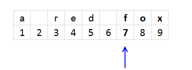
The functions used in most of the formulas on this web page are the SEARCH and FIND functions. They return a number based on the position of a text string in a value, see cell E3 on picture above. If the text string is not found the functions return #VALUE! error.
"fox" is found at character 7 in value "a red fox", see picture below.
The SEARCH function is case-insensitive and the FIND function is case-sensitive. You can replace these functions with each other if you are looking for a case-sensitive formula or vice versa.
The magic starts when you enter the formula as an array formula, this allows you to search an entire cell range for text strings.
Table of Contents
- Partial match and return multiple adjacent values
- Partial match and return multiple adjacent values corresponding to the number of matching values
- Partial match and return multiple adjacent values
- Partial match in multiple columns and return adjacent values
- Search and display all cells that contain all search strings
- Partial match and return value with highest level
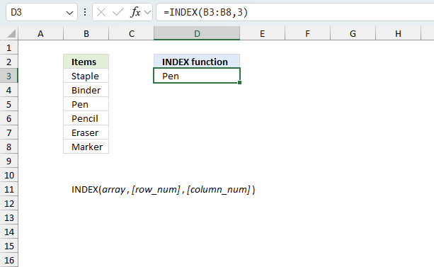
1. Search for a sub string in a column and return multiple corresponding values
John Paul asks:
I need a formula with no Macros – here an example of what I’m trying to do.
Column A contains:
Head-Phones-Sony
Black-Pen,Skilcraft
AAA-Batteries,24pk
Eraser,5pk
Ink-Pen,Fine-Point-Blue
Column B contains:
M412
M123
M784
M143
M572
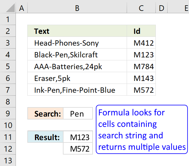
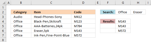
In Cell D1 I want to ENTER *Pen* and have it list all corresponding values which is Cell A2 & Cell A5
It sounds like a “Lookup one value with multiple corresponding values” but when I use a wildcard in my search it doesn’t work... Do you have a solution for it? Thank you
Answer:
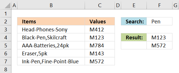
The picture below shows an array formula in cell F4 that searches cell range B3:B7 for the text string in cell F2 "Pen" and returns the adjacent value, on the same row, from column C.
Text string "Pen" is found in cell B4 and B7 so the formula returns adjacent value M123 and M572 to cell range F4:F5.
Array formula in cell F4:
1.1 Watch a video where I explain the formula above
Update 1/12/2021 - new dynamic array formula
Dynamic array formula in cell F4:
This formula contains the new FILTER function and works only for Excel 365 subscribers.
The following article explains how to look for values that contain two different text strings:
Recommended articles
This article demonstrates formulas that let you perform partial matches based on multiple strings and return those strings if all […]
This post explains how to look for strings in a cell value and return multiple corresponding values:
Recommended articles
Mr.Excel had a "challenge of the month" June/July 2008 about Wildcard VLOOKUP: "The data in column A contains a series […]
1.2 How to enter an array formula
- Copy formula
- Select cell E2
- Paste formula
- Press and hold Ctrl + Shift
- Press Enter
Recommended article
Recommended articles

Array formulas allows you to do advanced calculations not possible with regular formulas.
1.3 How to copy array formula
- Copy cell E2
- Paste to cell range E3:E4
1.4 Explaining array formula in cell E2
Step 1 - Search for a specific text string
SEARCH($E$1, $A$1:$A$5)
returns {#VALUE!;7;#VALUE!;#VALUE!;5}
Step 2 - Check if values in array contains a a number
ISNUMBER(SEARCH($E$1, $A$1:$A$5))
returns {FALSE; TRUE; FALSE; FALSE; TRUE}
Step 3 - Convert number to a row number
IF(ISNUMBER(SEARCH($E$1, $A$1:$A$5)), MATCH(ROW($A$1:$A$5), ROW($A$1:$A$5)))
returns {FALSE; 2; FALSE; FALSE; 5}
Step 5 - Filter n-th smallest row number in array
SMALL(IF(ISNUMBER(SEARCH($E$1, $A$1:$A$5)), MATCH(ROW($A$1:$A$5), ROW($A$1:$A$5))), ROW(A1))
returns 2.
Step 6 - Return adjacent value
INDEX($B$1:$B$5, SMALL(IF(ISNUMBER(SEARCH($E$1, $A$1:$A$5)), MATCH(ROW($A$1:$A$5), ROW($A$1:$A$5))), ROW(A1)))
returns "M123" in cell E2.
Recommended articles
Gets a value in a specific cell range based on a row and column number.
2. Search for a text string in a column and return multiple adjacent values corresponding to the number of matching values found
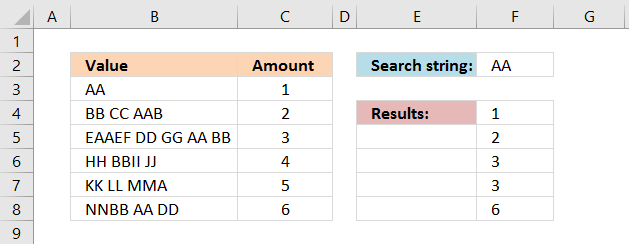
The picture above demonstrates an array formula that searches a cell range for a text string and returns the corresponding value on the same row as many times as the textstring is found in the value.
Example, cell B5 has value "EAAEF DD GG AA BB". Text string "AA" is found twice so the corresponding value on the same row is also returned twice (3).
Array formula in cell F4:
Get the Excel file
Search for a text string in a column and return multiple adjacent values corresponding to the number of matching values found.xlsx
3. Search for multiple text strings in a column and return multiple adjacent values
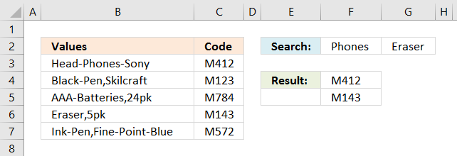
This array formula searches for both "Phones" and "Eraser" in column B, if at least one of them is found the corresponding value in column C is returned to F4 and F5.
Array formula in cell F4:
You can have more than two search strings if you like however they must be arranged horizontally (on the same row). If you want the search strings vertically (on the same column) use the TRANSPOSE function, like this: TRANSPOSE($F$1:$F$2)
Update 1/12/2021 - new dynamic array formula
Dynamic array formula in cell F4:
This formula contains the new FILTER function and works only for Excel 365 subscribers.
Get the Excel file
Search for multiple text strings in a column and return multiple adjacent values.xlsx
4. Search for a text string in multiple columns and return adjacent values
The picture above shows two search text strings in cell range G2:H2, the array formula in cell range G4:G7 searches in both columns B and C. If at least one text string is found the corresponding value in column D on the same row is returned to G4:G7.
Array formula in cell G4:
You can have more than two search strings if you like, however, they must be arranged horizontally (on the same row). If you want the search strings vertically (on the same column) use the TRANSPOSE function, like this: TRANSPOSE($G$1:$G$2)
5. Search and display all cells that contain all search strings
Jerome asks, in this blog post Search for multiple text strings in multiple cells in excel :
If the list of strings in column D was to increase to a large number e.g. 15, how would you tell excel to select the range of strings, so that you don't have to select each string "SEARCH($D$3" in the search parameter, as it seems is the case at the moment?
Array Formula in G3:
Change the following in order to add more conditions:
- cell reference $E$2:$E$3 if you want more conditions
- the number after the second equal sign =2 to as many conditions you have in the formula
- {1; 1} to as many conditions you have. For example, 4 conditions - {1; 1; 1; 1}
5.1 How to create an array formula
- Select cell F2
- Type formula in formula bar
- Press and hold Ctrl + Shift
- Press Enter
- Release all keys
5.2 Explaining formula in cell
Step 1 - Search for multiple strings
The SEARCH function allows you to find a string in a cell and it's character position. It also allows you to search for multiple strings in multiple cells if you arrange values in a way that works. That is why I use the TRANSPOSE function to transpose the values.
SEARCH(TRANSPOSE($E$2:$E$3), $B$3:$B$13)
returns {#VALUE!, 1; ... , 1}
Step 2 - Convert values into boolean values
The ISNUMBER function returns TRUE if value is number and FALSE for everything else including errors.
ISNUMBER(SEARCH(TRANSPOSE($E$2:$E$3), $B$3:$B$13))
returns {FALSE, TRUE;TRUE, ... , TRUE}
Step 3 - Convert boolean values
The MMULT function can't work with boolean values so we need to convert them to their numerical equivalents.
--(ISNUMBER(SEARCH(TRANSPOSE($E$2:$E$3), $B$3:$B$13)))
returns {0,1;1,... ,1}.
Step 4 - Add numbers in array row-wise
MMULT(--(ISNUMBER(SEARCH(TRANSPOSE($E$2:$E$3),$B$3:$B$13))),{1;1})=2
returns {FALSE; FALSE; FALSE; ... ; TRUE}.
Step 5 - Prevent duplicates in the list
The next COUNTIF function counts values based on a condition or criteria, the first argument has this cell reference: $G$2:G2. It expands as you copy the cell and paste to cells below.
(COUNTIF($G$2:G2, $B$3:$B$13)=0)
returns {TRUE; TRUE; TRUE; ... ; TRUE}
Step 6 - Multiply arrays
We apply AND logic if we multiply the arrays, this means both values must be TRUE in order to return TRUE.
(COUNTIF($G$2:G2, $B$3:$B$13)=0)* (MMULT(--(ISNUMBER(SEARCH(TRANSPOSE($E$2:$E$3), $B$3:$B$13))), {1; 1})=2)
returns {0;0;0;... ;1}
Step 6 - Divide 1 with array
The LOOKUP function ignores error values. Divide 1 with zero and we get #DIV/0! error.
1/((COUNTIF($G$2:G2, $B$3:$B$13)=0)* (MMULT(--(ISNUMBER(SEARCH(TRANSPOSE($E$2:$E$3), $B$3:$B$13))), {1; 1})=2))
returns {#DIV/0!; #DIV/0!; ... ; 1}.
Step 7 - Return values
LOOKUP(2, 1/((COUNTIF($G$2:G2, $B$3:$B$13)=0)*(MMULT(--(ISNUMBER(SEARCH(TRANSPOSE($E$2:$E$3), $B$3:$B$13))), {1; 1})=2)), $B$3:$B$13)
returns "FDB" in cell G3.
Get Excel *.xlsx file
Search and display all cells that contain all search strings.xlsx
6. Partial match and return value with highest level
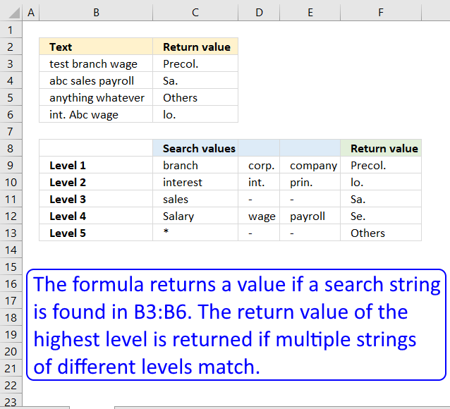
This article demonstrates a formula that searches a cell (partial match) based on values in a table and returns a value based on its position. The value with the highest level is returned if two matches are found.
For example, cell B3 in the above image contains the value "test branch wage", it matches both "branch" in cell C9 and "wage" in cell D12 however, only the corresponding value with the highest level is returned. "Level 1" is higher than "Level 2".
Value "branch" is on a higher level than the value "wage" and the corresponding value to "branch" is "Precol.", value "Precol." is returned to cell C3.
I have the matter to create a mega formula to categorize my list. For short example:A1: Cash in deposit (Branch A t/t)
A2: Borrowed from Corp. A
A3: Interest payment
A4: Int.penalty pmt
A5: Prin. Pmt
A6: Salary Pmt on April
A7: Sales abroad
A8: Branch C t/t
A9: Transferred from Company AA
A10: Mortgages to DD ltd
A11: Sal. Pmt on Mayand
at B1 cell, I create a formula as follows:=IF(COUNT(SEARCH({"branch","corp.", "company"},A1))>0,"Precol.", IF(COUNT(SEARCH({"interest","int.", "prin."},A1))>0,"lo.",IF(COUNT(SEARCH("sales", A1))>0,"Sa.",IF(COUNT(SEARCH({"sal.","Salary", "wage","payroll"},A1))>0,"Se.","Others"))))But, my formula is too long and too many parentheses. I want to shorten this formula or replace it with another. But how? Could you please solve my question? Thank you very much.Hung
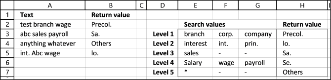
It looks like your formula has different levels with search words. The word found with the lowest level should be returned, leave the remaining.
Example 1, cell A2 contains "test branch wage". "branch" is found on level 1 (cell E3) and "wage" on level 4 (cell F6). However "branch" is on the lowest level of the two so Precol. (cell H3) is returned in cell B2.
Example 2, cell A3 contains "abc sales payroll". "sales" is a search string found on level 3 and "payroll" is on level 4. Level 3 is the lowest level so "Sa." (cell H5) is returned in cell B3.
Example 3, cell A4 contains"anything whatever" and no search value is found except the asterisk (*) on level 5. Text string "Others" (cell H7) is returned in cell B4.
How to enter an array formula
- Select cell B2.
- Type the formula above in the formula bar.
- Press and hold CTRL + SHIFT key.
- Press Enter.
If you did the above steps correctly excel automatically adds a beginning and ending curly bracket {array_formula} to the formula. Don't enter these characters yourself.
Explaining array formula in cell B2
You can easily follow along as I explain this array formula. Select cell B2 and go to "Formulas" on the ribbon, press with left mouse button on "Evaluate Formula" button. Press with mouse on "Evaluate" to go to next step.
Step 1 - Search for multiple text strings simultaneously
The SEARCH function returns the number of the character at which a specific character or text string is found. However, we are only interested if the string is found or not, this function is exactly what we need.
We are doing something strange with the SEARCH function below, we are not only using one string but multiple strings at once. That is why you see a cell range in the first argument.
SEARCH(find_text,within_text, [start_num])
SEARCH($E$3:$G$7,A2)
becomes
SEARCH({"branch","corp.","company";"interest","int.","prin.";"sales","-","-";"Salary","wage","payroll";"*","-","-"},"test branch wage")
and returns
{6, #VALUE!, #VALUE!; #VALUE!, #VALUE!, #VALUE!;#VALUE!, #VALUE!,#VALUE!; #VALUE!,13,#VALUE!; 1,#VALUE!, #VALUE!}
The SEARCH function returns an array with the same size as the cell range used in the first argument, see above.
$E$3:$G$7 is a cell range containing multiple columns and rows. An array with multiple columns and rows uses commas and semicolons as delimiting characters.
A comma is used as a delimiting character to separate values column by column and a semi colon is used to separate values row by row.
$E$3:$G$7 has three columns, E, F and G. The returning array above contains three values separated by two commas and then a semicolon, so the array has also three columns. The same with the number of rows in cell range $E$3:$G$7 and rows in array.
Step 2 - Look for numbers in array
A number indicates that the text string is found, an error #VALUE tells you that no search string is found. The ISNUMBER function converts numbers to TRUE and all other values including errors to FALSE.
ISNUMBER(value)
ISNUMBER(SEARCH($E$3:$G$7,A2))
becomes
ISNUMBER({6,#VALUE!,#VALUE!;#VALUE!, #VALUE!,#VALUE!;#VALUE!,#VALUE!,#VALUE!; #VALUE!,13,#VALUE!;1,#VALUE!,#VALUE!})
and returns {TRUE, FALSE, FALSE;FALSE, FALSE, FALSE;FALSE, FALSE, FALSE;FALSE, TRUE, FALSE;TRUE, FALSE, FALSE}
Step 3 - If text string is found return corresponding row number
The IF function returns one value if the logical test is TRUE and another value if the logical test is FALSE.
IF(logical_test, [value_if_true], [value_if_false])
IF(ISNUMBER(SEARCH($E$3:$G$7, A2)), MATCH(ROW($E$3:$G$7), ROW($E$3:$G$7)),"")
becomes
IF({TRUE, FALSE, FALSE;FALSE, FALSE, FALSE;FALSE, FALSE, FALSE;FALSE, TRUE, FALSE;TRUE, FALSE, FALSE}, MATCH(ROW($E$3:$G$7), ROW($E$3:$G$7)), "")
becomes
IF({TRUE, FALSE, FALSE;FALSE, FALSE, FALSE;FALSE, FALSE, FALSE;FALSE, TRUE, FALSE;TRUE, FALSE, FALSE}, {1; 2; 3; 4; 5}, "")
and returns
{1,"","";"","","";"","","";"",4,"";5,"",""}
Step 4 - Extract smallest row number
The MIN function allows you to retrieve the smallest number in a cell range.
MIN(number1, [number2], ...)
MIN(IF(ISNUMBER(SEARCH($E$3:$G$7, A2)), MATCH(ROW($E$3:$G$7), ROW($E$3:$G$7)), ""))
becomes
MIN({1,"","";"","","";"","","";"",4,"";5,"",""})
and returns 1.
Step 5 - Return value using row number
The INDEX function returns a value from a cell range, you specify which value based on a row and column number.
INDEX(array,row_num,[column_num])
INDEX($H$3:$H$7, MIN(IF(ISNUMBER(SEARCH($E$3:$G$7, A2)), MATCH(ROW($E$3:$G$7), ROW($E$3:$G$7)), "")))
becomes
INDEX($H$3:$H$7, 1)
becomes
INDEX({"Precol.";"lo.";"Sa.";"Se.";"Others"}, 1)
and returns Precol. in cell B2.
Search and return multiple values category
This article demonstrates formulas that let you perform partial matches based on multiple strings and return those strings if all […]
This article demonstrates three different ways to filter a data set if a value contains a specific string and if […]
Excel categories
83 Responses to “Partial match and return multiple adjacent values”
Leave a Reply
How to comment
How to add a formula to your comment
<code>Insert your formula here.</code>
Convert less than and larger than signs
Use html character entities instead of less than and larger than signs.
< becomes < and > becomes >
How to add VBA code to your comment
[vb 1="vbnet" language=","]
Put your VBA code here.
[/vb]
How to add a picture to your comment:
Upload picture to postimage.org or imgur
Paste image link to your comment.
Can you do this by displaying an adjacent column instead of the column that was searched?
if that is not possible then can you do this formula by having List (A2:A12) start at A3 and go to A13?
okay I figured it out! thanks and I love your site!!
Man how long have you been working with excel?... i have just 2 years and I didn't have the slightest idea (till know ) you can do this only with formulas, I usually solve this kind of issues with VBA macros.
What can you recommend me to be able to do this? review each one of the formulas and its examples , or reading a lot of excel books or what?
I have learned a lot just by starting an excel blog.
Review others formulas and reading books is a good start. Enjoy what you are doing and solutions come easily into mind.
Oscar,
Thanks again. Would you help me with replaced search string1 with replace string1 and search string2 with replace string2....etc.... thanks,
James
Here is a much shorter alternate
=INDEX(B$1:B$5,SMALL(IFERROR(IF(SEARCH(F$1,A$1:A$5),ROW(B$1:B$5)),""),ROW(A1)))
@sam,
I am guessing Oscar did not post your formula version because it uses IFERROR which is only available on XL2007 and above. The formula in the blog article will work with XL2003 (I don't have earlier versions of Excel to know about them) in addition to XL2007 and above, so Oscar's formula is a more universal one.
sam,
thanks for your contribution!
Maybe I should explain why I use MATCH(ROW($A$1:$A$5), ROW($A$1:$A$5)) and not ROW($A$1:$A$5).
MATCH(ROW($A$1:$A$5), ROW($A$1:$A$5)) returns an array of row numbers regardless of the size and position of the cell range, named range or dynamic named range.
Example,
ROW($A$5:$A$11) returns {5, 6, 7, 8, 9, 10, 11}.
MATCH(ROW($A$5:$A$11), ROW($A$5:$A$11)) returns {1, 2, 3, 4, 5, 6, 7}
I am trying to use your formula but ran into an issue. I am using Excel 2013 and stuck at this step (Step 3). MATCH(ROW($A$1:$A$5),ROW($A$1:$A$5) returns FALSE for cells not containing target text (Pen), which is fine, but returns #N/A for cells containing target text; therefore, not converting to row numbers. Any help would be much appreciated. Thank you.
I meant IF(ISNUMBER(SEARCH($E$1, $A$1:$A$5)), MATCH(ROW($A$1:$A$5), ROW($A$1:$A$5))) returns FALSE for cells not containing target text (Pen), but returns #N/A for cells containing target text.
Koji,
did you enter the formula as an array formula?
Thank you, Oscar. That solved it.
Great! although it's unable to correctly find the 02590 string. What could it be?
Andres,
02590?
Can you provide an example?
Hello Oscar,
My worksheet is failing not yours (blush). I put new strings on yours and it works just as I expected. Need to dig into it a bit more, he he.
Thanks for your valuable attention and congrats for your portal.
- Andres.
Hello Oscar,
Here I have an example (https://www.yourfilelink.com/get.php?fid=830240) for the functions of this page. As you can see in this example I am telling the spreadsheet to find what is in cell A3 but it show the content for row 3775 instead. I used hardcoded ranges aswell as named ranges with no change. When I put the content of the Example.xls spreadsheet in your spreadsheet it works but refuses to work in mine, perhaps due because I am using Excel 2003 but I am not fully convinced.
Thank you!
- Andres.
Andres,
Use this array formula in cell K7:
Hi Oscar,
I need to combine row and text columns into one "text" and suppress errors. Excel complaints that I exceeded the nested formulas.
Much appreciated..
Sorry Oscar,
Forgot to mention, only one search string is required, and may contain letters and numbers.
Best regards.
Carl,
combine row and text columns into one "text" and suppress errors
Can you provide an example?
Hi Oscar,
I am trying to do a search on string with possible more than 1 match and return values horizontally. I tried to use your helpful tips however I got error. Do it limited on # of rows? I only have 5244 rows to be search.
Here is an example. Any help would be greatly appreciated.
Sheet 1 Column A:
2088
2088_5252
2085_5258
Sheet 2 Column A:
2088
2085
Expected result on Sheet 2:
Column A
2088
2085
Column B
2088
2085_5258
Column C
2088_5252
Columns go on depending on the # of matches
Thank you so much.
Joey,
Get the Excel *.xlsx file
Find-text-string-and-return-multiple-values-horizontally.xlsx
Hi, I'm trying to do the following search.
I'd
Column A
86(b)
61(c)
Column B
92(b)
and table
86(a) 1
86(b) 2
86(c) 3
92(a) 1
92(b) 2
92(c) 3
61(a) 1
61(b) 2
61(c) 3
expected result
in one cell, search a1:b2 for 61(?) to return the value from the table which is 3 here,
in 2nd cell, search a1:b2 for 86(?) to return the value from the table which is 2 here, and
in 3rd cell, search a1:b2 for 92(?) to return the value from the table which is 2.
Han Hoe Liw,
Get the Excel *.xlsx file
Han-Hoe-Liw.xlsx
Read post:
Lookups in a related table (array formula)
I have two types of cells in the worksheet. Some are with green background and some are with plain white background. Some of these cells have a string of syntax in regular expression "ABC".
Each cell could have 1 or more strings according to regular expression above separated by ","(comma).
Could experts guide me on a formula
How to count the number of "ABC" in a every green/white cells to have an over all total in a given range.
For example, if cell 1 have 3 strings, cell 2 has 5 strings. The total is 8
Hi Oscar,
Very useful code. Is it possible to remove the #NUM! that you get? I have tried to use the following code without success:
{=IF(ISERROR($E$2); ""; INDEX($B$1:$B$5; SMALL(IF(ISNUMBER(SEARCH($E$1; $A$1:$A$5)); MATCH(ROW($A$1:$A$5); ROW($A$1:$A$5))); ROW(A1))))}
David
This array formula works in Excel 2007 and above:
=IFERROR(INDEX($B$1:$B$5, SMALL(IF(ISNUMBER(SEARCH($E$1, $A$1:$A$5)), MATCH(ROW($A$1:$A$5), ROW($A$1:$A$5))), ROW(A1))), "")
Just wanted to express my thanks for these solutions! Helped me out immensely today.
jchew,
Thank you for commenting.
HI OScar
I need 2 adjacent result displayed.
Thnaks
amman
aman,
Try this array formula:
=INDEX($B$1:$C$5, SMALL(IF(ISNUMBER(SEARCH($E$1, $A$1:$A$5)), MATCH(ROW($A$1:$A$5), ROW($A$1:$A$5))), ROW(A1)),COLUMN(A1))
The two adjacent values are in column B and C.
Hi ,
Can anyone help in getting a formula for below .
My requirement : In a given columns list(A1:A14) i need to search for a name from that column and print the total of payee in another column ( example for Jack, print total of Jack amount which is from row C and print it(F5) cell as shown in below .). I have tried with above formula INDEX but i cannot able get the expected results .
A B C D E F
1 Payee Date Amount
2 Jack 10 My results should look like
3 steve 39 Name Total
4 John 150
5 Jack 20 Tom 23
6 steve 200 Jack 30
7 Todd 34 Steve 239
8 Tom 23 Todd 132
9 Todd 98
10
11
12
13
14
Kumar
Kumar,
Formula in cell B12:
=SUMIF($A$2:$A$9,A12,$C$2:$C$9)
Thank you Oscar , it worked!. appreciate your help.
Hi Oscar, i was redirected here after posting a question on another webpage and after manipulating the formulas here. I have the answer i wanted. You are awesome! Thanks!
Tip to the others: I came here looking for a 'loose' vlookup. To further make it 'looser', add an element of NON-case sensitive, I used the function SEARCH instead of FIND. Hope this helps you!
Hi Oscar,
Thank you so much for these forumlas. I have been using this one a lot.
=INDEX($B$1:$B$6, SMALL(IF(COUNTIF($E$2:E2, $B$1:$B$6)(LEN($A$1:$A$6)-LEN(SUBSTITUTE($A$1:$A$6, $E$1, "")))/LEN($E$1), MATCH(ROW($A$1:$A$6), ROW($A$1:$A$6)), ""), 1))
Is there a way to take it a step further and only shot unique values using the frequency formula?
CODE
AA_100 John S
AA_100
AA_100
AA_200
AA_200
AA_200
Apologies I had not finished that post before it sent!
Here is an example of my data and what I'd hope the formula would return:
https://postimg.org/image/l61e8j593/9321549a/
Thinking on it SumProduct and frenquency wouldn't work as they don't return text and that's what I'm after.
Let me know if you need more information, thanks in advance!
Samantha,
maybe you are looking for this?
Array formula in cell E4:
=INDEX($A$4:$A$15, SMALL(IF(ISNUMBER(SEARCH($C$1,$A$4:$A$15))*NOT(COUNTIF($E$3:E3, $A$4:$A$15)), MATCH(ROW($A$4:$A$15), ROW($A$4:$A$15)), ""), 1))
[UPDATE]
This post has a smaller better formula.
Filter unique distinct values where adjacent cells contain search string
Thank you very much! This is exactly what I'm after.
Oscar,
Thanks for providing a walkthru of the "search" functionality. I have another lookup for multiple values, but not finding it elsewhere yet.
I want to use that formula, along with another criteria that must be true in order to return a value
Name.......Status.....Job...Date
John.......Done.......cc1...05/05/2014
Rick.......Done.......05....05/06/2014
John,Sam...Done.......z35...05/04/2014
John,Rick..Incomplete.d3d...""
Rick,Sam...Canceled...j3j...05/09/2014
bob,john...Done.......0O0...05/11/2014
I would use the search to find each row with "John" (dropdown links to Name), but how would I further constrain the list so that only "Done" is returned??
Result
Job...Date
cc1...05/05/2014
z35...05/04/2014
0O0...05/11/2014
Thanks in advance.
Andy
Hi Oscar, one question master..
i have this in sheet1
a b c d e f c
1ten P1 $3 P2 $4
2
3
in other sheet i have a vlookup searching for "ten", but im have two providers, in the sheet2 im going to put "P1" in one C5, and other cell the vlookup "=vlookup(C5,sheet1!a1:c:3, ( here mi problem ) for "ten" im want the result of the P1 but maybe next day im want the P2 price, how its de correct formula.. ?
greetings.
Dear Oscar, in trying to train myself on all things Excel, I ran into a problem while trying to return the values horizontally instead of vertically. I tried to teak the array based on some other formula but to no avail. Would you be so kind as to point a little grasshopper in the right direction? Thank you kindly.
Oscar
Need your assistant in writing a formula for searching a string within sting in a column. Very similar to above examples but the difference is that I have 3000 rows (Sheet A) for array columns and about 7000 rows (SheetB) for search criteria. Here is an example of data.
Sheet A
Column A Column B Roll over bed with extra frame 17-1
Queen room with suite 89-0
King room with kitchen and photo frame 14-0
Sheet B
Column A Column D (Expected results)
Frame 17-1 14-0
Kitchen 14-0
Room 89-0 14-0
Hi Oscar
I have a very unnusual request. i need to put in a formula that will return the results in a cell (alphabetical) as a total. eg:
Column A
Detail: cant clear LA1
0
FALSE
FALSE
this information is in one column. I need to have a "total" that will pull through the information that is not 0 or FALSE
Note, only one cell in the column will show info that is not 0 or FALSE
Hi,
I was trying to use this but my case is a little bit different.
I have 2 sheets:
- In sheet 1, i have two columns, one with the long text and the other one with the result
- In sheet 2, i also have two columns, and in first column i have the ID's and on second the description.
So, i want to search the ID's in from sheet 2 in the long text from sheet 1 and insert the description associated to ID in the first sheet.
Take the example:
Sheet 1:
A1 - My ID is unique.
B1 - (blank)
Sheet 2:
A1 - ID
B1 - Identification
Since there's ID on text in sheet1!A1, i want that sheet1!B1 = sheet2!B2. Which means this should also be "Identification"
Could you please help?
Let's say I have following two col of data
BB CC AAB 2
DD GG AA BB 3
HH BBII JJ 4
KK LL MMA 5
NNBB AA DD 6
in any other cell I want to write a formula such that->if you find "LL" any text string in col 1, then return the corresponding number in col B, which is 5. What that formula be? Thanks for your help.
Im trying to solve this problem. I,ve read your posts and they all look great, but what if you dont know what you are looking for? ie searching from a list!
The formula I have searches for words in a text strings, starting with A1, then adds categories from a large list of categories in a table on ANOTHER WORKSHEET 'Dynamic Categories Lists' , depending on the words found in the A1 string. The formula is in B1. The amount of data is huge 19,000 text strings in Column A.
For examples the text string might say:
A B C
1 dog has black spots Dalmatian
2 dog is tall Large Dog
My formula searches for "black spots" and returns " Dalmatians " to B1
My formula searches for " dog is tall" - my formula searches " tall " and return " large dogs" to B2
Formula in B1 is:
=PROPER(IFERROR(LOOKUP(1E+100,SEARCH('Dynamic Categories Lists'!$A$1:$A$1000,A1),'Dynamic Categories Lists'!$A$1:$A$1000),""))
'Dynamic Categories Lists' (DIFFERENT WORKSHEET)
A B
1 Search Word to Find Categories: List Paste
2 black spots Dalmatian
3 tall Large Dog
4 short Small Dog
5 -1000 MORE -1000 MORE
My problem is I need to find the 2nd, 3rd, 4th occurrences
Example
A B C D
1 dog has black spots Dalmatian
2 dog is tall Large Dog
3
4 dog has black spots and is tall Dalmatian Large Dog
A4 "dog has black spots and is tall" I want the formula to return "Dalmatian" & "large dog" to B3
Any help would be appreciated. I have searched heaps of threads and haven’t been able to find the answer!
Thanks for sharing your thoughts. What really I am after:
I put my monthly bank statement in excel. It has cols with date, description of the charges, and the amount debited form my account (to make it simple). There are, say 100 such tractions lines in a given month. What I want, In a different work sheet, in “one” cell I want I want to write a formula to find how much did I spend in store, say, Staples. If a find a line with the this matching word, get the data from next col and keep summing up until last row. Is that too much to ask from excel? I know Ecel is a very powerful spread sheet and I am sure there must be an answer to this. I just could not find it yet. Any help from anybody would be appreciated.
Miah Baset,
Is that too much to ask from excel?
Definitely not, use a pivot table:
https://www.excel-easy.com/data-analysis/pivot-tables.html
How would I combine this formula:
=INDEX($B$1:$B$5,SMALL(IF(ISNUMBER(SEARCH($E$1,$A$1:$A$5)),MATCH(ROW($A$1:$A$5),ROW($A$1:$A$5))),ROW(A1)))
With a sum formula, so that the multiple instances are summarized into 1 cell.
Example:
A B C
LOOKUP SUM
TX 25 *TX* 110
Lewisville TX 35 *MI* 60
Dallas TX 50
Detroit MI 10
Grand Rapids MI 20
MI 30
How would I combine this formula:
=INDEX($B$1:$B$5,SMALL(IF(ISNUMBER(SEARCH($E$1,$A$1:$A$5)),MATCH(ROW($A$1:$A$5),ROW($A$1:$A$5))),ROW(A1)))
With a sum formula, so that the multiple instances are summarized into 1 cell.
Example:
A------ B-----C-----D---------E
------------------LOOKUP----- SUM
TX---25---------- *TX*------- 110
Lewisville TX---35-*MI*------ 60
Dallas TX--- 50
Detroit MI--- 10
Grand Rapids MI--- 20
MI--- 30
SUMPRODUCT function
Thanks You! Please solve my query here: I have a value in a cell A1 which contains:
M4.CTC.VA03.Verify Sales Documents.v2 [14294], MSUP.CTC.VA03.Verify Sales Documents.v2 [14957], MSUP.CTC.VA03.Verify Sales Documents.v2 [15019], MSUP.CTC.VA03.Verify Sales Documents.v3 [15156]
I would like to have a value in Cell B as: 14294;14957;15019;15156
Basically, it should look for a text "[" and then return all characters after untill reaches "]".
Please help.
Hi, I'm trying to extract two values from a table.
I have multiple rows of data:
Column1 Column2 Column3 Column4 Column5 Column6 Column7 Column8 PAloc1 PAloc2 PBloc1 PBloc2
FALSE FALSE PAlocBaseline FALSE PAlocOuterAD FALSE PBlocInnerDeuce PBlocLongLong PAlocABaseline #N/A PBlocInnerDeuce PBlocInnerDeuce
FALSE FALSE PAlocBaseline FALSE FALSE PAlocTramAD PBlocInnerDeuce PBlocLongLong PAlocABaseline PAlocBaseline PBlocInnerDeuce PBlocInnerDeuce
FALSE FALSE PAlocBaseline FALSE PAlocOuterAD FALSE PBlocInnerDeuce PBlocLongLong PAlocABaseline PAlocBaseline PBlocInnerDeuce PBlocInnerDeuce
FALSE FALSE PAlocBaseline FALSE FALSE PAlocTramAD PBlocInnerDeuce PBlocLongLong PAlocABaseline PAlocBaseline PBlocInnerDeuce PBlocInnerDeuce
FALSE FALSE PAlocInnerAD FALSE PAlocLongLong FALSE FALSE PBlocBaseline PAlocAInnerAD PAlocInnerAD PBlocBaseline PBlocBaseline
FALSE PAlocLongLong FALSE PAlocInnerAD FALSE FALSE FALSE PBlocDeep PAlocALongLong PAlocLongLong PBlocDeep PBlocDeep
FALSE PAlocLong PAlocOuterAD FALSE FALSE FALSE PBlocOuterDeuce FALSE PAlocALong PAlocLong PBlocOuterDeuce PBlocOuterDeuce
FALSE FALSE PAlocBaseline PAlocInnerAD FALSE FALSE
I need the first instance of where PAloc shows up to populate in PAloc1 and the second instance to populate in PAloc2. The data varies as to when each instance show up.
I tried:
=INDEX(F6:Q6, SMALL(IF(ISNUMBER(SEARCH($F$2, F6:Q6)), MATCH(ROW(F6:Q6:$A$5), ROW(F6:Q6))), ROW(A6)))
Where F2 is "paloc"
It sounds like a “Lookup one value with multiple corresponding values” but when I use a wildcard in my search it doesn’t work... Do you have a solution for it?
I cannot successfully find the sum total of all the amounts for a specific Code (whats the total for R02 or R04, etc). I would love to hear any suggestions
Code Amount
R02 $200
R02 $200
R04 $200
R04 $200
R04 $200
R04 $200
R04 $200
R04 $200
R04 $200
R04 $200
R04 $200
R04 $200
R04 $200
R04 $200
R05 $200
R05 $200
R05 $200
R05 $200
R11 $200
R11 $200
R11 $200
R11 $200
R11 $200
R11 $200
R11 $200
R11 $200
R11 $200
R16 $300
R16 $300
R16 $300
R16 $200
R16 $300
R16 $300
R16 $300
R16 $300
R16 $300
Check out the SUMPRODUCT function.
H 5
H 5
I 6
G 4
H 5
G 4
G 4
J 7
H 5
G 4
G 4
F 3
I 6
G 4
Hey oscar,
If column A has for text like color code above and if D=1 and Z=23. how to get those value in adjacent cell using formula. I have tried IF Isnumber Search but not getting result.
I am using following formula.
=IF(ISNUMBER(SEARCH("D",c3)),"1",IF(ISNUMBER(SEARCH("E",c3)),"2",IF(ISNUMBER(SEARCH("F",c3)),"3",IF(ISNUMBER(SEARCH("G",c3)),"4",IF(ISNUMBER(SEARCH("H",c3)),"5",IF(ISNUMBER(SEARCH("I",c3)),"6",IF(ISNUMBER(SEARCH("J",c3)),"7",IF(ISNUMBER(SEARCH("K",c3)),"8",IF(ISNUMBER(SEARCH("L",c3)),"9",IF(ISNUMBER(SEARCH("M",c3)),"10",IF(ISNUMBER(SEARCH("N",c3)),"11",IF(ISNUMBER(SEARCH("O",c3)),"12",IF(ISNUMBER(SEARCH("P",c3)),"13",IF(ISNUMBER(SEARCH("Q",c3)),"14",IF(ISNUMBER(SEARCH("R",c3)),"15",IF(ISNUMBER(SEARCH("S",c3)),"16",IF(ISNUMBER(SEARCH("T",c3)),"17",IF(ISNUMBER(SEARCH("U",c3)),"18",IF(ISNUMBER(SEARCH("V",c3)),"19",IF(ISNUMBER(SEARCH("W",c3)),"20",IF(ISNUMBER(SEARCH("X",c3)),"21",IF(ISNUMBER(SEARCH("Y",c3)),"22",IF(ISNUMBER(SEARCH("Z",c3)),"23")))))))))))))))))))))))
Shardul
Try this formula:
=CODE(C3)-67
i have lookup array
A1 (anil) B1 (12)
A2(Singh) b2(13)
c1(Amit) c2(14)
looking for G1( Anil Singh Amit)
return value should be in G2(12 13 14)
if it possible kindly help me out
i have thousands of this type queries
if G1 ( Singh Anil Amit)
return value should be (13 12 14)
if G1 ( Singh Anil Amit)
return value should be (13 12 14)
if G1( Singh Anil Amit)
return value should be in G2(13 12 14)
Hi Oscar,
I have used the formula you have provided above
=INDEX($C$3:$C$7, SMALL(IF(ISNUMBER(SEARCH($F$2, $B$3:$B$7)), MATCH(ROW($B$3:$B$7), ROW($B$3:$B$7))), ROWS($A$1:A1)))
I have done this To search through a table of patients for if a procedure was aborted and why it was aborted. So it will spit out the reason a patient procedure was aborted. In some cases the procedure was aborted for the same reason. Using your formula the array is simply repeating the same reasons. Is there a way to modify the formula that if there is a repeat it will not add it as a row in my array. See what the formula spits out below:
1st Anchor Pull out
TSP Unsuccessful
TSP Unsuccessful
1st Anchor Pull out
1st Anchor Pull out
so it successfully searched for aborted in one column and then returned the adjacent row that had the reason in it. If the reason repeats I just would like it not to repeat the reason in my final array. Is this possible?
Thank you,
Rachel
Rachel,
Try these formulas:
Formula in cell H3:
=INDEX(C$3:C$8, SMALL(IF(ISNUMBER(SEARCH($F$3, $B$3:$B$8)), MATCH(ROW($B$3:$B$8), ROW($B$3:$B$8)), ""), ROWS($A$1:A1)))
Formula in cell I3:
=IFNA(INDEX($D$3:$D$8, MATCH(1, (COUNTIF($I$2:I2, $D$3:$D$8)=0)*($C$3:$C$8=H3), 0)), "")
Get the Excel *.xlsx file
Search-for-a-text-string-and-return-multiple-adjacent-values_Rachel.xlsx
G8 work bro, can we get the results in column wise rather then rows ??
It works horizontally as well. Use the same formulas as above but enter it in cell H2.
Then copy cell H2 and paste it to I2 and as far as needed.
=LOOKUP(2, 1/((COUNTIF($G$2:G2, $B$3:$B$13)=0)*(MMULT(--(ISNUMBER(SEARCH(TRANSPOSE($E$2:$E$3), $B$3:$B$13))), {1; 1})=2)), $B$3:$B$13)
The bolded cell reference above is important in order to get values horizontally: $G$2:G2
You need to change it so it points to the cell to the left of the current cell. Example, if you are going to enter the formula in cell L5 then change the cell reference to $K$5:K5.
Hi,
I have a list of movies into a column, and I want to list all cells that contains a specific word/s.
It is similar than doing a filter and looking for some chain "text", and I want to know and list all the cells that match that chain text.
Is that possible?
Joaquin,
The easiest way to list all cells containing "text" would be to apply a filter.
1. Select any cell in your data set.
2. Go to tab "Home".
3. Press with left mouse button on "Sort & Filter" button.
4. Press with left mouse button on "Filter".
The header names now have arrows.
1. Press with left mouse button on an arrow based on the column you want to filter.
2. Press with left mouse button on "Text Filters".
3. Press with left mouse button on "Contains..".
4. Type the text string you want to match.
5. Press with left mouse button on ok button.
The data is now filtered.
Sir,
I tried the excel file and it works well. but when I modify the number of rows I want to search from 3 to 10. it stops working. when the file is received the formula appears in {}, when I edit this goes away and the formula stops working.
Sir,
I opened the excel file it works well. but when I modify the number of rows I want to search from 3 to 10. it stops working. when the file is received the formula appears in {}, when I edit this goes away and the formula stops working. let me know how to solve it
Balachandra
The {} tells you that the formula is an array formula and not a regular formula. You need to enter the formula as an array formula if you edit an array formula.
1. Press and hold CTRL + SHIFT simultaneously.
2. Press Enter.
3. Release all keys.
split this into multiple rows
2 Unit Cattle Feed Supplement Vimicon 3 kg Rs. 750 10 Unit Drumstick PKM 1 50 gm Rs. 260 10 Unit Drumstick PKM 1 50 gm Rs. 260 Scheme price per pkt 12 rs discount 6 Unit Fodder Grass Bijankur-BB2 50 gm Rs. 360 4 Unit Fodder Grass Alamdar 51 1 kg Rs. 675 4 Unit Fodder Grass Alamdar 51 1 kg Rs. 675 1 Unit Fodder Grass Bijankur-BB2 50 gm Rs. 360
result should like this
2 Unit Cattle Feed Supplement Vimicon 3 kg Rs. 750
10 Unit Drumstick PKM 1 50 gm Rs. 260
10 Unit Drumstick PKM 1 50 gm Rs. 260 Scheme price per pkt 12 rs discount
6 Unit Fodder Grass Bijankur-BB2 50 gm Rs. 360
4 Unit Fodder Grass Alamdar 51 1 kg Rs. 675
4 Unit Fodder Grass Alamdar 51 1 kg Rs. 675
1 Unit Fodder Grass Bijankur-BB2 50 gm Rs. 360
Then it should assign a number specific word from a above eg vimicon assign a number 28 without using if condition from a table
Hello Oscar, can you provide Arrayformula on google sheets. I need to search numbers in one column against another then display values in an adjacent column. I can share my spreadsheet with you
Thanks for helping us !
I want to get similar data but only for the exact match of the cells,
say for eg.,
one
two
four
twenty one
five
thirty one
and I want to pull data corresponds to one only not for twenty one.
Can you please help on that ?
Manibala
Read this article: 5 easy ways to VLOOKUP and return multiple values
I need assistance with a search formula. I have leases with term periods and at the end of a term period in column J is an "X" I use this in formulas to review upcoming leases ending in 12 months on another tab. I want to return any and all renewal options available UNDER any row that contains the x (but from columns b, c, and d). I have over 50 leases on different tabs - so the placement of x indicating the term of the lease varies from tab to tab and also will change as leases are updated, but is always within a range of J10:J29.
This message is in response to the initial query raised by John Paul titled 'Search for a text string and return multiple adjacent values'.
My problem is trying to contain all the multiple returned values in one cell (separated by comma) rather than list the various returned values in vertical/horizontal adjacent cells.
I am able to obtain the first returned match by using the formula; =VLOOKUP("*"&Value&"*",Tab!$RangeA$,column number,FALSE)
However what I really require is all the returned values contained in one cell (separated by comma)... Any help would be gratefully appreciated.
Array formula:
TEXTJOIN, IF, ISNUMBER, and SEARCH functions.
Hi Oscar, your site is amazing!
Referring to "Search for a text string in multiple columns and return adjacent values"
Is there are way to only return the values which fulfill both search strings?
Thank you!
Yes, there is.
Excel 365 subscribers can use this smaller dynamic array formula:
It contains the new FILTER function that you can read about here: FILTER function
Is there a way to change TRANSPOSE($E$2:$E$3) from a column of data to a row?
I've tried $D$2:$E$2 and neither work in the cell but in the Function Arguments box it shows the expected value.
I think it is an issue with circular references but Excel can't show the problem.
Hi Oscar,
Thank you for posting these amazing tutorials! I am using this formula below to search for the subject I want to look up (let's say pens in cell K1). Then I also have many other things (erasers, rulers in cell L1, M1) to look up, so how can I apply this formula to the other ones? I tried applying this formula by dragging the right corner of the box, but because the formula is locked, the results will appear the same as for K1 for the L1 and M1 search. Is there a way to overcome this issue other than manually change the lookup cells in the search function?
=INDEX($A$1:$A$151,SMALL(IF(ISNUMBER(SEARCH($K$1,$C$1:$C$151)),MATCH(ROW($C$1:$C$151),ROW($C$1:$C$151))),ROW(A1)))