How to use VLOOKUP/XLOOKUP with multiple conditions
I will in this article demonstrate how to use the VLOOKUP function with multiple conditions. The function was not built for these circumstances, however, I will demonstrate a few workarounds and also explain how they work.
There is a file for you to get at the very end of this article.
Table of Contents
-
VLOOKUP examples
- VLOOKUP function with two conditions applied to two columns (AND logic)?
- VLOOKUP function with two conditions applied to two columns (OR logic)?
- VLOOKUP function with many conditions applied to one column (OR logic)?
- Can we use VLOOKUP with multiple lookup values?
- VLOOKUP across multiple columns?
- Can you concatenate VLOOKUP results?
- How to use VLOOKUP with dates?
- What if I don't have the lookup column in the left-most column?
- VLOOKUP - Select column using a drop-down list
- Why do I want to convert the data set to an Excel Table?
- VLOOKUP in a filtered Excel Table and return multiple values
- VLOOKUP of three columns to pull a single record
- XLOOKUP - two conditions in two columns (AND logic)?
- XLOOKUP - two conditions in two columns (OR logic)?
- XLOOKUP - multiple conditions in one column (OR logic)?
- Can we use XLOOKUP with multiple lookup values?
- XLOOKUP across multiple columns?
- Can you concatenate XLOOKUP results?
- How to use XLOOKUP with dates?
- What if I don't have the lookup column in the left-most column?
- XLOOKUP of three columns to pull a single record
- FILTER records based on three conditions
XLOOKUP examples
Return multiple instances
1.1 How to use the VLOOKUP function with two conditions (AND logic)?
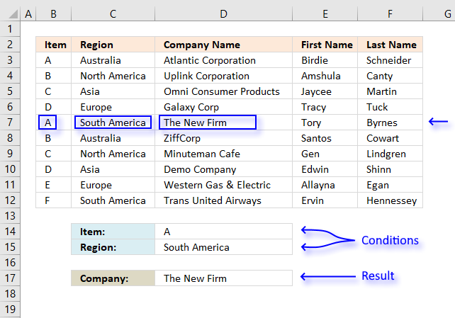
The image above shows a data set in cell range B2:F12, the VLOOKUP function in cell D16 looks for both a value in column B and another value in column C. If both values match a third value on the same row is retrieved from column D and shown in cell D17.
AND logic means that the VLOOKUP function retrieves only if both conditions match.
Can you combine the IF function and the VLOOKUP function?
Yes, you can, in fact, it is the easiest way to VLOOKUP using two or more conditions.
Array formula in D17:
To enter an array formula press and hold CTRL + SHIFT simultaneously, then press Enter once. Release all keys.
The formula bar now shows the formula enclosed with curly brackets telling you that you entered the formula successfully. Don't enter the curly brackets yourself.
Explaining formula in cell D17
I recommend you use the "Evaluate Formula" feature in Excel to examine calculations step by step.
Select cell D17, go to tab "Formulas" on the ribbon and press with left mouse button on the "Evaluate Formula" button.
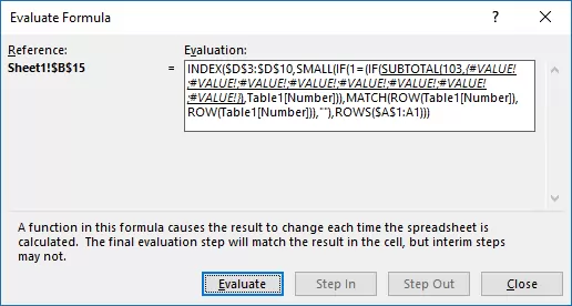
(The formula shown in the above image is not the formula used in this article.)
Press with left mouse button on "Evaluate" button to see the next step in the formula calculations.
Step 1 - Filter records
The IF function filters records that match the value in cell D15, all remaining records are blank. The IF function has three arguments: IF(logical_test, [value_if_true], [value_if_false])
The logical_test argument is C3:C12=D15, it checks if the values in column C are equal to the condition in cell D15. TRUE is returned if it is equal and FALSE if not equal.
IF(C3:C12=D15, B3:F12, "")
returns {"","","",... ,"Hennessey"}
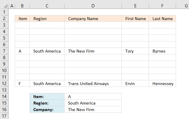
This array has commas and semicolons as delimiting characters, the picture below shows the array in cell range B3:F12. It is now obvious that the IF function has filtered records containing ony the condition.
Step 2 - VLOOKUP value and return value from column to cell D16
VLOOKUP(D14,IF(C3:C12=D15,B3:F12,""),3,FALSE)
returns "The New Firm" in cell D16.
1.2 How to use the VLOOKUP function with two conditions applied to two columns (OR logic)?
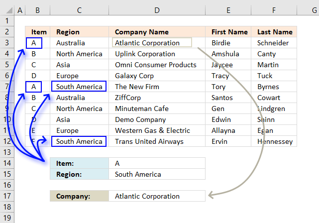
This example demonstrates a formula that returns a value from a record that matches at least one of the two conditions, that is why it is called OR logic.
It becomes quite quickly obvious that the VLOOKUP function is not built for more advanced criteria, I am not using the VLOOKUP function in this example, to keep the formula as small as possible.
Array formula in cell D17:
To enter an array formula press and hold CTRL + SHIFT simultaneously, then press Enter once. Release all keys.
The formula bar now shows the formula enclosed with curly brackets telling you that you entered the formula successfully. Don't enter the curly brackets yourself.
If you are looking for a non-array formula here is one:
This formula returns a value from the last matching record contrary to the first formula above that returns a value from the first matching record.
Explaining formula in cell D17
Step 1 - First condition
The first condition is specified in cell D14, to compare that value with the values in cell range B3:B14 I use the equal sign. It is a logical operator that returns TRUE or FALSE after the evaluations is made.
We are performing multiple calcualtions in one cell and this is the reason we need to enter this as an array formula.
B3:B12=D14
returns {TRUE; FALSE; FALSE; ... ; FALSE}
Step 2 - Second condition
C3:C12=D15
returns {FALSE; FALSE; FALSE; ... ; TRUE}
Step 3 - Add arrays to apply OR logic
The plus sign adds the two arrays row-wise, TRUE + TRUE = 2, TRUE + FALSE = 1 and FALSE + FALSE = 0
((B3:B12=D14)+(C3:C12=D15))>0
returns {TRUE; FALSE; FALSE; ... ; TRUE}
Step 4 - Identify the position
The MATCH function, as it is set up in this example, returns the relative position of the first found matching value based on an exact match.
MATCH(TRUE,((B3:B12=D14)+(C3:C12=D15))>0,0)
returns 1.
Step 5 - Return the corresponding value
The INDEX function returns a value based on a row and column number.
INDEX($D$3:$D$12, MATCH(TRUE, ((B3:B12=D14)+(C3:C12=D15))>0, 0))
returns "Atlantic Corporation" in cell D17.
1.3 How to use the VLOOKUP function with many conditions applied to one column (OR logic)?
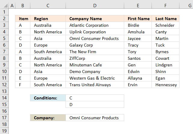
This example demonstrates how to use multiple conditions and the formula returns a value from the first record that matches any of the conditions.
The following formula does not use the VLOOKUP function, it is possible to build such formula but it will be complicated and much larger than needed.
Array formula in cell D17:
To enter an array formula press and hold CTRL + SHIFT simultaneously, then press Enter once. Release all keys.
The formula bar now shows the formula enclosed with curly brackets telling you that you entered the formula successfully. Don't enter the curly brackets yourself.
Explaining formula in cell D17
Step 1 - Check values that match
The COUNTIF function counts values that equal a condition, however, it can also count multiple conditions but we must enter this formula as an array formula in order to calculate multiple values in one cell.
COUNTIF(D14:D15, B3:B12)>0
returns
{0;0;1;1;0;0;1;1;0;0}.
This array has as many values as there are values in cell range B3:B12, the values also corresponds to B3:B12. 0 (zero) indicates that the value is not equal to "C" or "D" and 1 shows that the value is equal to "C" or "D".
Step 2 - Find the position of the record
The MATCH function, as it is set up in this example, returns the relative position of the first found matching value based on an exact match.
MATCH(1, COUNTIF(D14:D15, B3:B12), 0)
returns 3. The first value that is equal to 1 is in 3rd position in the array.
Step 3 - Return corresponding value
The INDEX function returns a value based on a row and column number, the cell range is in a column only, we don't need to specify the column number.
INDEX($D$3:$D$12, MATCH(1, COUNTIF(D14:D15, B3:B12), 0))
returns "Omni Consumer Products".
1.4 How to use VLOOKUP function with multiple lookup values?
This example demonstrates how to use multiple lookup values in the VLOOKUP function, the lookup values are in cell D14 and D15.
The lookup values are found in row 5,6,9 and 10 but only the corresponding values from row 5 and 6 are returned, that is how the VLOOKUP function is supposed to work. If you need to extract multiple values based on a condition read this: 5 easy ways to VLOOKUP and return multiple values
Array formula in cell D14:D15:
This is an array formula, it returns multiple values. We need to enter it in multiple cells at once, here is how to do it.
Select cell range D14:D15, press with left mouse button on in the formula bar to see the prompt. Copy and paste above array formula to formula bar.
To enter an array formula press and hold CTRL + SHIFT simultaneously, then press Enter once. Release all keys.
The formula bar now shows the formula enclosed with curly brackets telling you that you entered the formula successfully. Don't enter the curly brackets yourself.
The VLOOKUP function demonstrated above has two lookup values which is fine as long as you enter it in as many cells as there are lookup values.
The downside with this formula is that it only extracts one return value per lookup value, read this article: Vlookup with 2 or more lookup criteria and return multiple matches
1.5 VLOOKUP across multiple columns?
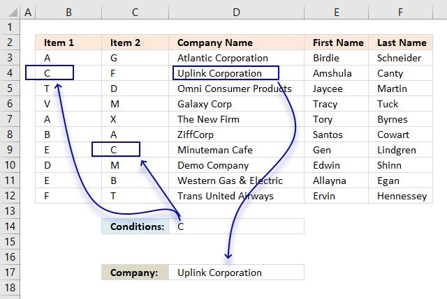
Unfortunately, the VLOOKUP function can't look in other columns than the left-most column in a cell range. We need to use other functions to accomplish that.
The image above demonstrates an array formula in cell D17 that returns a value from column D (Company Name) if the corresponding value on the same row in column B or C matches the specified value in cell D17.
Array formula in cell D17:
To enter an array formula press and hold CTRL + SHIFT simultaneously, then press Enter once. Release all keys.
The formula bar now shows the formula enclosed with curly brackets telling you that you entered the formula successfully. Don't enter the curly brackets yourself.
Explaining formula in cell D17
Step 1 - Compare values to the lookup value
The equal sign lets you check if a cell value is equal to another value, the difference with this setup is that it compares a cell value to a cell range.
In this case B3:C12, this is fine as long as you enter the formula as an array formula. The formula performs multiple calcualtions in one cell, the result is an array containing boolean values, TRUE or FALSE.
B3:C12=D14
returns {FALSE,FALSE; TRUE,... ,FALSE}
Step 2 - Replace boolean values with corresponding row number
The IF function allows you to change the array based on if the logical expression returns TRUE or FALSE.
IF(B3:C12=D14,MATCH(ROW(B3:B12),ROW(B3:B12)),"")
returns {"",""; 2,... ,""}
Step 3 - Extract the smallest row number
The MIN function returns the samllest number from an cell range or array.
MIN(IF(B3:C12=D14,MATCH(ROW(B3:B12),ROW(B3:B12)),"")
returns 2.
Step 4 - Return value
The INDEX function returns a value from a cell range or array based on a row and column number. Our example has only a single column so the column number is not needed.
INDEX($D$3:$D$12,MIN(IF(B3:C12=D14,MATCH(ROW(B3:B12),ROW(B3:B12)),"")))
returns "Uplink Corporation".
1.6 Can you concatenate VLOOKUP results?
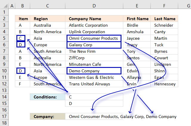
No, you can't concatenate multiple return values from a VLOOKUP function. It will only return one instance. This example shows how to concatenate multiple values using multiple conditions using the TEXTJOIN, IF and COUNTIF functions.
Array formula in cell D17:
To enter an array formula press and hold CTRL + SHIFT simultaneously, then press Enter once. Release all keys.
The formula bar now shows the formula enclosed with curly brackets telling you that you entered the formula successfully. Don't enter the curly brackets yourself.
Explaining formula in cell D17
Step 1 - Determine which records match the conditions
The COUNTIF function counts values equal a condition or in this case multiple conditions.
COUNTIF(D14:D15,B3:B12)
returns {0; 0; 1; ... ; 0}.
Step 2 - Replace array with values
The IF function allows you to change the array based on if the logical expression returns TRUE or FALSE.
IF(COUNTIF(D14:D15,B3:B12),D3:D12,"")
returns
{"";"";"Omni Consumer Products";... ;""}
Step 3 - Concatenate values
The TEXTJOIN function allows you to concatenate a cell range or array, you can choose the delimiting character and if you want to ignore blank values.
TEXTJOIN(", ",TRUE, IF(COUNTIF(D14:D15,B3:B12),D3:D12,""))
returns "Omni Consumer Products, Galaxy Corp".
1.7 How to use VLOOKUP with dates?
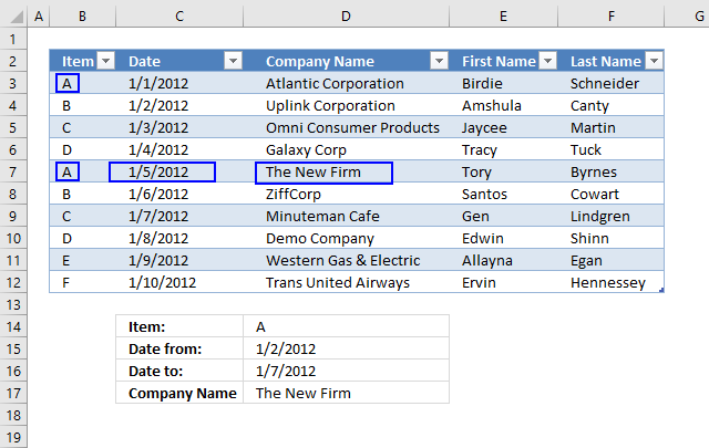
This example shows how to VLOOKUP using a condition, start and end date. The formula returns a value from the first record that matches all three conditions.
Array formula in cell C5:
To enter an array formula press and hold CTRL + SHIFT simultaneously, then press Enter once. Release all keys.
The formula bar now shows the formula enclosed with curly brackets telling you that you entered the formula successfully. Don't enter the curly brackets yourself.
Explaining formula in cell C5
Step 1 - Identify rows with dates larger than the start date
This logical expression checks whether the dates in column Date are bigger (later) than the start date in cell C3.
Table3[Date]>=C3
returns {FALSE; TRUE; TRUE;... ; TRUE}
Step 2 - Identify rows with dates smaller than the end date
The following logical expression checks whether the dates in column Date are smaller (earlier) than the end date in cell C3.
Table3[Date]<=C4
returns {TRUE;TRUE;TRUE;... ;FALSE}
Step 3 - Multiply arrays
We want to know if both conditions are met, to do that we must multiply the arrays. TRUE * TRUE = TRUE (1), TRUE * FALSE = FALSE (0), FALSE * FALSE = FALSE (0)
(Table3[Date]>=C3)*(Table3[Date]<=C4)
returns {0;1;1;1;1;1;1;0;0;0}
Step 4 - Filter records that match
The IF function filters records that match both conditions.
IF((Table3[Date]>=C3)*(Table3[Date]<=C4),Table3,"")
returns {"","","",... ,""}.
Step 5 - VLOOKUP using the array
The VLOOKUP function uses the array returned from the IF function and looks for the lookup value in the left-most column in the array.
VLOOKUP(C2,IF((Table3[Date]>=C3)*(Table3[Date]<=C4),Table3,""),3,FALSE)
returns "The New Firm"
1.8 What if I don't have the lookup column in the left-most column?

The VLOOKUP function can only look for values in the first column of the table_array. The formula below demonstrates how to do a lookup in any table column and return a value from any table column.
The INDEX and MATCH function is more versatile than VLOOKUP and it is easier to apply more conditions if needed, however, it still can only return one value even if there are more records that match. The INDEX, SMALL and IF function can return multiple values, read this article: 5 easy ways to VLOOKUP and return multiple values
Formula in cell C3:
Learn more about the INDEX and MATCH functions:
Recommended articles
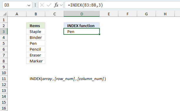
Gets a value in a specific cell range based on a row and column number.
Recommended articles
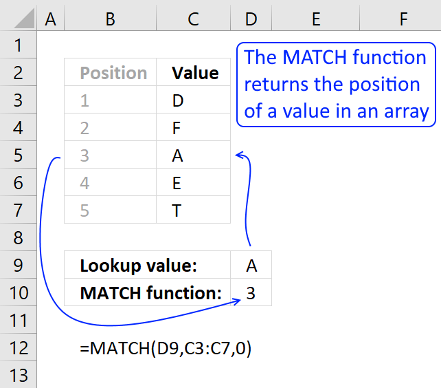
Identify the position of a value in an array.
becomes
INDEX(Table4[Item],4)
becomes
INDEX({"A"; "B"; "C"; "D"; "A"; "B"; "C"; "D"; "E"; "F"},4)
and returns D in cell C3.
1.9 VLOOKUP - Select column using a drop-down list

The worksheet shown above lets you select the column using a drop-down list from which you want the return value, this way you don't need to edit the formula when you need data from another column.
Array formula in cell C4:
How to create the drop down list in cell B4
- Select cell B4
- Go to "Data" tab
- Press with left mouse button on "Data Validation" button
- Select "List" i the drop down list
- Select source: =$C$8:$E$8

- Press with left mouse button on OK
Explaining formula in cell C4
Step 1 - Find the relative position
The MATCH function returns the relative position of an item in an array that matches a specified value in a specific order.
Function syntax: MATCH(lookup_value, lookup_array, [match_type])
MATCH(B4, Table2[#Headers], 0)
returns 3.
Step 2 - Logical test
The equal sign is a logical operator, it lets you compare a value to another value in an Excel formula. The result is a boolean value, TRUE or FALSE.
You can use the equal sign to compare a value to a cell range of values as well.
Table2[Region]=C3
returns {FALSE; FALSE; FALSE; ... ; TRUE}
Step 3 - Filter values based on a condition
The IF function returns one value if the logical test is TRUE and another value if the logical test is FALSE.
Function syntax: IF(logical_test, [value_if_true], [value_if_false])
IF(Table2[Region]=C3, Table2, "")
returns {"","","",... ,"Hennessey"}
Step 4 - Perform a lookup
The VLOOKUP function lets you search the leftmost column for a value and return another value on the same row in a column you specify.
Function syntax: VLOOKUP(lookup_value, table_array, col_index_num, [range_lookup])
VLOOKUP(C2, IF(Table2[Region]=C3, Table2, ""), MATCH(B4, Table2[#Headers], 0), FALSE)
returns "The New Firm".
1.10 Why do I want to convert the data set to an Excel Table?

If you convert your cell range to a table you can add or remove as many records to the Excel table as you want and the cell reference in the formula is automatically adjusted.
Use the table name and table column name in the VLOOKUP function to achieve this, see the formula bar in the picture above.
How to convert a cell range to an Excel defined Table?
- Select any cell in your data set.
- Go to tab "Insert" on the ribbon.
- Press with left mouse button on "Table" button to open a dialog box.
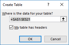
- Enable "My table has headers".
- Press with left mouse button on OK.
Learn more about excel tables:
Recommended articles
An Excel table allows you to easily sort, filter and sum values in a data set where values are related.
1.11 VLOOKUP in a filtered Excel Table and return multiple values
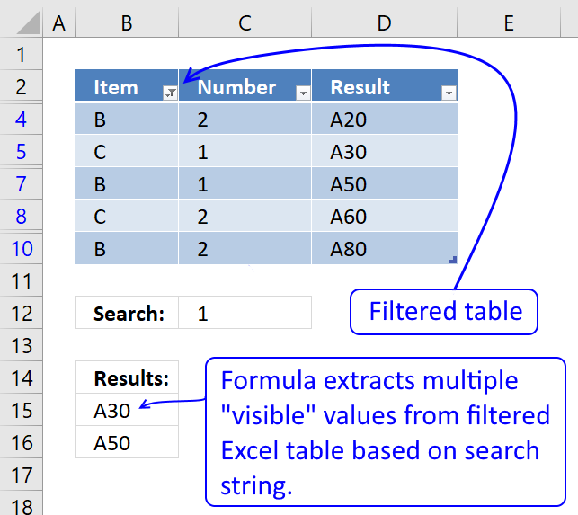
This section describes how to search filtered values in an Excel defined Table using a condition given in cell 12 and return multiple values. Some rows are hidden because of Excel Table filters, I am not using the VLOOKUP function in this formula.
Excel 365 dynamic array formula in cell B15:
Array Formula in cell B15:
How to create an array formula
- Copy (Ctrl + c) and paste (Ctrl + v) array formula into formula bar.

- Press and hold Ctrl + Shift.
- Press Enter once.
- Release all keys.
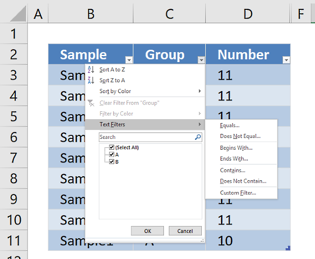
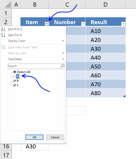
Filter table
Let's remove all A's from item column. Press with left mouse button on black arrow near Item header. Deselect A. Press with left mouse button on OK.
Explaining formula in cell B15
Step 1 - Create array
This step is necessary in order to be able to use the SUBTOTAL function in the next step. The ROW function returns row numbers based on a cell reference.
The MATCH function converts the row number array to an array that starts with 1.
OFFSET(Table1[Number], MATCH(ROW(Table1[Number]), ROW(Table1[Number]))-1, 0, 1)
returns {2; 1; 2; 1; 2; 1; 2}.
Step 2 - Which values are shown in the Filtered Excel table
The SUBTOTAL(103, array) counts the number of values that are not empty.
SUBTOTAL(103, OFFSET(Table1[Number], MATCH(ROW(Table1[Number]), ROW(Table1[Number]))-1, 0, 1))
returns {0; 1; 1; 0; 1; 1; 0; 1}
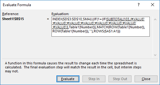
This array may look weird, the array in the SUBTOTAL function has 7 values and the result array has 8 values, how is it possible? This is, however, what you get if you convert the functions to constants by selecting them using and then pressing F9.
If you examine the formula using the "Evaluate Formula" tool you get the following array: {#VALUE!; #VALUE!; #VALUE!; #VALUE!; #VALUE!; #VALUE!; #VALUE!; #VALUE!}
Even more confusing. This is what I think is going on. The OFFSET function actually returns an array of arrays, like this { {2}; {1}; {2}; {1}; {2}; {1}; {2} }
Then the SUBTOTAL function returns an array that indicates if the value is shown in the filtered table or not. 0 (zero) means not shown and 1 is visible.
{0; 1; 1; 0; 1; 1; 0; 1} meaning row 3, 6 and 9 are hidden in the filtered table.
Step 3 - Convert array to actual values
The IF function has three arguments, the first one must be a logical expression. If the expression evaluates to TRUE then one thing happens (argument 2) and if FALSE another thing happens (argument 3).
IF(SUBTOTAL(103, OFFSET(Table1[Number], MATCH(ROW(Table1[Number]), ROW(Table1[Number]))-1, 0, 1)), Table1[Number])
returns {FALSE; 2; 1; FALSE; 1; 2; FALSE; 2}
Step 4 - Match values to condition specified in cell C12
IF($C$12=(IF(SUBTOTAL(103, OFFSET(Table1[Number], MATCH(ROW(Table1[Number]), ROW(Table1[Number]))-1, 0, 1)), Table1[Number])), MATCH(ROW(Table1[Number]), ROW(Table1[Number])), "")
returns {""; ""; 3; ""; 5; ""; ""; ""}
Step 5 - Extract k-th smallest row number
To be able to return a new value in a cell each I use the SMALL function to extract row numbers from smallest to largest.
The ROWS function keeps track of the numbers based on an expanding cell reference. It will expand as the formula is copied to the cells below.
SMALL(IF($C$12=(IF(SUBTOTAL(103, OFFSET(Table1[Number], MATCH(ROW(Table1[Number]), ROW(Table1[Number]))-1, 0, 1)), Table1[Number])), MATCH(ROW(Table1[Number]), ROW(Table1[Number])), ""), ROWS($A$1:A1))
returns 3.
Step 6 - Return value based on row number
The INDEX function returns a value based on a cell reference and column/row numbers.
INDEX(Table1[Result], SMALL(IF($C$12=(IF(SUBTOTAL(103, OFFSET(Table1[Number], MATCH(ROW(Table1[Number]), ROW(Table1[Number]))-1, 0, 1)), Table1[Number])), MATCH(ROW(Table1[Number]), ROW(Table1[Number])), ""), ROWS($A$1:A1)))
returns A30 in cell B15.
1.12. VLOOKUP of three columns to pull a single record
The VLOOKUP is designed to get a value in a specified column, based on a lookup value. It can't evaluate multiple conditions and also return multiple values from the same row where the lookup value is found.
The formula below demonstrates a formula that is able to do this, read section2, and 3 below if you are using Excel 365. Those formulas are much easier to create and understand.
Array formula in B18:
Update! The VLOOKUP can process multiple conditions in some cases: How to use VLOOKUP/XLOOKUP with multiple conditions and return multiple values, here is how:
Array formula in B18:
Copy cell B18 and paste to cells to the right as far as needed.
How to enter an array formula
To enter an array formula, type the formula in a cell then press and hold CTRL + SHIFT simultaneously, now press Enter once. Release all keys.
The formula bar now shows the formula with a beginning and ending curly bracket telling you that you entered the formula successfully. Don't enter the curly brackets yourself.
Explaining formula
Step 1 - Return 1 if all conditions are met
The COUNTIFS function calculates the number of cells across multiple ranges that equals all given conditions.
Function syntax: COUNTIFS(criteria_range1, criteria1, [criteria_range2, criteria2]…)
COUNTIFS($B$14, $B$3:$B$11, $C$14, $D$3:$D$11, $D$14, $E$3:$E$11)
returns {0; 0; 0; 0; 1; 0; 0; 0; 0}
Step 2 - Find the relative position
The MATCH function returns the relative position of an item in an array that matches a specified value in a specific order.
Function syntax: MATCH(lookup_value, lookup_array, [match_type])
MATCH(1, COUNTIFS($B$14, $B$3:$B$11, $C$14, $D$3:$D$11, $D$14, $E$3:$E$11), 0)
becomes
MATCH(1, {0; 0; 0; 0; 1; 0; 0; 0; 0}, 0)
and returns 5.
Step 3 - Create a sequence of numbers from 1 to n
The COLUMNS function calculates the number of columns in a cell range.
Function syntax: COLUMNS(array)
COLUMNS($A$1:A1)
returns 1.
When cell B18 is copied to cell C18 the formula changes to COLUMNS($A$1:B1) and returns 2. The number grows by 1 for each cell.
Step 4 - Get value
The INDEX function returns a value or reference from a cell range or array, you specify which value based on a row and column number.
Function syntax: INDEX(array, [row_num], [column_num])
INDEX($B$3:$F$11,MATCH(1, COUNTIFS($B$14, $B$3:$B$11, $C$14, $D$3:$D$11, $D$14, $E$3:$E$11), 0), COLUMNS($A$1:A1))
returns "Y".
Get Excel *.xlsx file
vlookup of three columns to pull a single record.xlsx
2.1 XLOOKUP function with two conditions applied to two columns (AND logic)?

Excel 365 formula in cell D17:
Explaining formula
Step 1 - First condition
The equal sign is a logical operator, it lets you compare a value to another value in an Excel formula. The result is a boolean value, TRUE or FALSE.
You can use the equal sign to compare a value to a cell range of values as well.
B3:B12=D14
returns {TRUE; FALSE; FALSE; ... ; FALSE}.
Step 2 - Second condition
C3:C12=D15
returns {FALSE; FALSE; FALSE; ... ; TRUE}.
Step 3 - Apply AND logic
The parentheses let you control the order of operation. We need to calculate the comparisons before we multiply the arrays.
(B3:B12=D14)*(C3:C12=D15)
returns {0;0;0;0;1;0;0;0;0;0}.
Boolean values, when multiplied, return their numerical equivalents. TRUE - 1 and FALSE is 0 (zero).
Here is why AND logic is created when we multiply boolean values, both values must be TRUE in order to return TRUE.
TRUE * TRUE = 1 (TRUE)
TRUE * FALSE = 0 (FALSE)
FALSE * FALSE = 0 (FALSE)
Step 4 - Evaluate XLOOKUP function
The XLOOKUP function search one column for a given value, and return a corresponding value in another column from the same row.
Function syntax: XLOOKUP(lookup_value, lookup_array, return_array, [if_not_found], [match_mode], [search_mode])
XLOOKUP(1,(B3:B12=D14)*(C3:C12=D15),D3:D12)
returns "The New Firm".
2.2 XLOOKUP function with two conditions applied to two columns (OR logic)?

This example shows how to perform lookups in two different columns using two different lookup values respectively. The first record that meets at least one of two conditions is a match, in this example, row 3 is a match and the corresponding value in column D is returned.
Excel 365 formula in cell D17:
Explaining formula
Step 1 - First condition
The equal sign is a logical operator, it lets you compare a value to another value in an Excel formula. The result is a boolean value, TRUE or FALSE.
You can use the equal sign to compare a value to a cell range of values as well.
D14=B3:B12
returns {TRUE; FALSE; FALSE; ... ; FALSE}
Step 2 - Second condition
D15=C3:C12
returns {FALSE; FALSE; FALSE; ... ; TRUE}.
Step 3 - Apply OR logic
The parentheses let you control the order of operation. We need to calculate the comparisons before we multiply the arrays.
(D14=B3:B12)+(D15=C3:C12)
returns {1; 0; 0; 0; 2; 0; 0; 0; 0; 1}.
The plus sign performs addition between two numbers and also boolean values.
TRUE + TRUE = 2 (TRUE)
TRUE + FALSE = 1 (TRUE)
FALSE + FALSE = 0 (FALSE)
Boolean values, when added, are converted to their numerical equivalents.
TRUE - All numbers except zero.
FALSE - 0 (Zero)
Step 4 - Check if numbers are larger than or equal to 1
The larger than sign is a logical operator that lets you compare numbers and also text values if needed. The result is a boolean value, TRUE or FALSE.
((D14=B3:B12)+(D15=C3:C12))>=1
Step 5 - Evaluate XLOOKUP function
The XLOOKUP function search one column for a given value, and return a corresponding value in another column from the same row.
Function syntax: XLOOKUP(lookup_value, lookup_array, return_array, [if_not_found], [match_mode], [search_mode])
XLOOKUP(TRUE, ((D14=B3:B12)+(D15=C3:C12))>=1, D3:D12)
returns "Atlantic Corporation".
2.3 XLOOKUP - multiple conditions in one column (OR logic)?

This example demonstrates the XLOOKUP function using multiple conditions, however, it returns only a single value from the same row where any of the lookup values are found.
This example shows that the first condition is found before the second condition and the corresponding value on the same row is found in cell D5.
Excel 365 formula in cell D17:
Explaining formula
Step 1 - Count conditions in each value
The COUNTIF function calculates the number of cells that is equal to a condition.
Function syntax: COUNTIF(range, criteria)
COUNTIF(D14:D15, B3:B12)
returns {0; 0; 1; 1; 0; 0; 1; 1; 0; 0}.
Step 2 - Lookup based on array
The XLOOKUP function search one column for a given value, and return a corresponding value in another column from the same row.
Function syntax: XLOOKUP(lookup_value, lookup_array, return_array, [if_not_found], [match_mode], [search_mode])
XLOOKUP(1, COUNTIF(D14:D15, B3:B12), D3:D12)
returns "Omni Consumer Products".
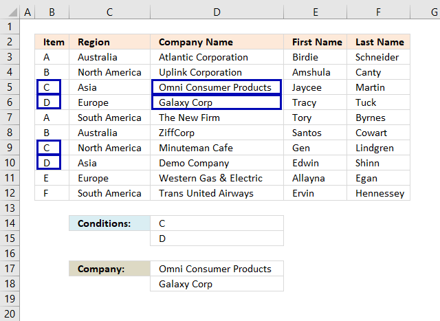
2.4 Can we use XLOOKUP with multiple lookup values?

This example demonstrates the XLOOKUP function also using multiple conditions, however, it returns as many values as there are conditions as long as they match the lookup values..
This example shows the condition in cell D14 is found in cell B5 and the corresponding value in cell D5 is returned to cell D17. The second condition in cell D15 is found in cell B6 and the corresponding value in cell D6 is returned to cell D18.
Excel 365 dynamic formula in cell D17:
Explaining formula
The XLOOKUP function lets you lookup multiple values in a single formula, the result is an Excel 365 dynamic array that spills values to cells below automatically.
Evaluate XLOOKUP function
The XLOOKUP function search one column for a given value, and return a corresponding value in another column from the same row.
Function syntax: XLOOKUP(lookup_value, lookup_array, return_array, [if_not_found], [match_mode], [search_mode])
XLOOKUP(D14:D15, B3:B12, D3:D12)
returns {"Omni Consumer Products"; "Galaxy Corp"}.
2.5 XLOOKUP across multiple columns?

This example performs a lookup across multiple columns using a single lookup value, a value from the first match on the same row is returned, in this example, cells D3:D12.
Excel 365 formula in cell D17:
Explaining formula
Step 1 - First column B
The equal sign is a logical operator, it lets you compare a value to another value in an Excel formula. The result is a boolean value, TRUE or FALSE.
You can use the equal sign to compare a value to a cell range of values as well.
B3:B12=D14
returns {FALSE; TRUE; FALSE; ... ; FALSE}.
Step 2 - Second column C
C3:C12=D14
returns {FALSE; FALSE; FALSE; ... ; FALSE}.
Step 3 - Apply OR logic
The plus sign adds numbers in an Excel formula, it also performs OR logic for boolean values and their numerical equivalents.
TRUE + TRUE = TRUE
TRUE + FALSE = TRUE
FALSE + FALSE = FALSE
OR logic means that at least one boolean value is TRUE in order to return TRUE.
TRUE - Any number except 0 (zero)
FALSE - 0 (zero)
The parentheses lets you control the order of operation, we need to compare the values before we add arrays.
(B3:B12=D14)+(C3:C12=D14)
returns {0;1;0;... ;0}.
Step 4 - Evaluate XLOOKUP function
The XLOOKUP function search one column for a given value, and return a corresponding value in another column from the same row.
Function syntax: XLOOKUP(lookup_value, lookup_array, return_array, [if_not_found], [match_mode], [search_mode])
XLOOKUP(1,(B3:B12=D14)+(C3:C12=D14),D3:D12)
returns "Uplink Corporation".
2.6 Can you concatenate XLOOKUP results?

You can concatenate results from the XLOOKUP function, this example demonstrates an XLOOKUP function that lookups two different values, and the results are concatenated using the TEXTJOIN function.
Excel 365 formula in cell D17:
Explaining formula
Step 1 - Lookup two different values
The XLOOKUP function search one column for a given value, and return a corresponding value in another column from the same row.
Function syntax: XLOOKUP(lookup_value, lookup_array, return_array, [if_not_found], [match_mode], [search_mode])
XLOOKUP(D14:D15,B3:B12,D3:D12)
returns {"Omni Consumer Products"; "Galaxy Corp"}.
Step 2 - Join values
The TEXTJOIN function combines text strings from multiple cell ranges.
Function syntax: TEXTJOIN(delimiter, ignore_empty, text1, [text2], ...)
TEXTJOIN(", ",TRUE, XLOOKUP(D14:D15,B3:B12,D3:D12))
returns "Omni Consumer Products, Galaxy Corp".
2.7 How to use XLOOKUP with dates?

This example shows how to use a date range, Excel table, and a condition in the XLOOKUP function. The cell reference (structured reference) to the Excel Table doesn't change even if you add or delete rows in the table.
Excel 365 formula:
Explaining formula
Step 1 - Find dates equal or larger than the start date specified in cell D15
The less than and larger than characters are logical operators, they return TRUE or FALSE if the condition is met or not.
Table35[Date]>=D15
returns {FALSE; TRUE; TRUE; ... ; TRUE}.
Step 2 - Find dates equal or larger than the end date specified in cell D16
Table35[Date]<=D16
returns {TRUE; TRUE; TRUE; ... ; FALSE}.
Step 3 - Find records matching condition specified in cell D14
D14=Table35[Item]
returns {TRUE; FALSE; FALSE; ... ; FALSE}.
Step 4 - Apply AND logic
The parentheses let you control the order of operation. We need to calculate the comparisons before we multiply the arrays.
(Table35[Date]>=D15)*(Table35[Date]<=D16)*(D14=Table35[Item])
The asterisk character lets you multiply boolean values. When multiplied boolean values return their numerical equivalents. TRUE - 1 and FALSE is 0 (zero).
TRUE * TRUE = 1 (TRUE)
TRUE * FALSE = 0 (FALSE)
FALSE * FALSE = 0 (FALSE)
Both values must be TRUE in order to return TRUE.
returns {0; 0; 0; 0; 1; 0; 0; 0; 0; 0}
Step 5 - Evaluate XLOOKUP function
The XLOOKUP function search one column for a given value, and return a corresponding value in another column from the same row.
Function syntax: XLOOKUP(lookup_value, lookup_array, return_array, [if_not_found], [match_mode], [search_mode])
XLOOKUP(1, (Table35[Date]>=D15)*(Table35[Date]<=D16)*(D14=Table35[Item]), Table35[Company Name])
returns "The New Firm".
2.8 What if I don't have the lookup column in the left-most column?

The XLOOKUP function lets you use any lookup column contrary to the VLOOKUP function that requires the leftmost column as the lookup column.
This example demonstrates a lookup column in column C, the leftmost column is column B in the data set.
Formula in cell D15:
Evaluate XLOOKUP function
The XLOOKUP function search one column for a given value, and return a corresponding value in another column from the same row.
Function syntax: XLOOKUP(lookup_value, lookup_array, return_array, [if_not_found], [match_mode], [search_mode])
XLOOKUP(D14, C3:C12, D3:D12)
returns "Atlantic Corporation".
2.9. XLOOKUP of three columns to pull a single record
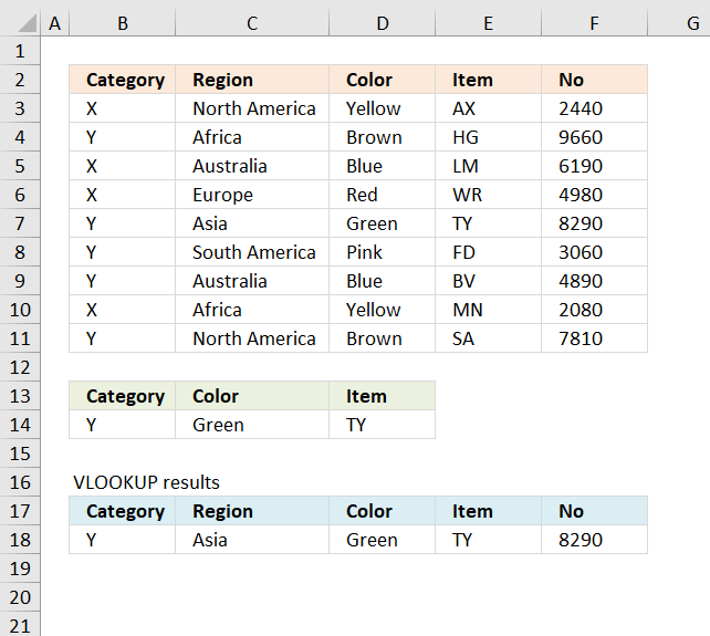
This example shows how easy it is to use the XLOOKUP function, the conditions are in cells B14, C14, and D14 respectively. The XLOOKUP function returns the record and spills values to the right as far as needed.
Excel 365 formula in cell B18:
Explaining formula
Step 1 - First condition
The equal sign is a logical operator, it lets you compare value to value in an Excel formula. It also works with arrays, the result is an array of boolean values TRUE and FALSE.
The first condition is specified in cell B14, it returns TRUE if a match is found.
B3:B11=B14
returns {FALSE; TRUE; ...: TRUE}.
Step 2 - Second condition
The second condition is specified in cell C14, it is compared to all values in cells D3:D11.
D3:D11=C14
becomes
returns {FALSE; FALSE; ... ; FALSE}.
Step 3 - Third condition
The third condition is specified in cell D14, the value is compared to all values in cells D3:D11.
E3:E11=D14
becomes
returns {FALSE; FALSE; ... ; FALSE}.
Step 4 - Control order of operation and the perform AND logic
The parentheses lets you control the order of operation, it is important that the comparisons are performed before multiplying the arrays.
The asterisk character lets you multiply numbers and boolean values in an Excel formula. Boolean values are converted into their numerical equivalents. TRUE - 1 and FALSE - 0 (zero).
(B3:B11=B18)*(D3:D11=C14)*(E3:E11=D14)
returns {0; 0; 0; 0; 1; 0; 0; 0; 0}.
Step 5 - Get a record based on specified conditions
The XLOOKUP function search one column for a given value, and return a corresponding value in another column from the same row.
Function syntax: XLOOKUP(lookup_value, lookup_array, return_array, [if_not_found], [match_mode], [search_mode])
XLOOKUP(1,(B3:B11=B18)*(D3:D11=C14)*(E3:E11=D14),B3:F11)
returns {"Y", "Asia", "Green", "TY", 8290}.
3. FILTER records based on three conditions
The FILTER function lets you extract all records that match the given conditions, this example returns one record. Only one record match all given conditions.
Excel 365 formula in cell B18:
Explaining formula
Step 1 - First condition
The equal sign is a logical operator, it lets you compare value to value in an Excel formula. It also works with arrays, the result is an array of boolean values TRUE and FALSE.
The first condition is specified in cell B14, it returns TRUE if a match is found.
B3:B11=B14
returns {FALSE; TRUE; ...: TRUE}.
Step 2 - Second condition
The second condition is specified in cell C14, it is compared to all values in cells D3:D11.
D3:D11=C14
returns {FALSE; FALSE; ... ; FALSE}.
Step 3 - Third condition
The third condition is specified in cell D14, the value is compared to all values in cells D3:D11.
E3:E11=D14
returns {FALSE; FALSE; ...; FALSE}.
Step 4 - Control order of operation and the perform AND logic
The parentheses lets you control the order of operation, it is important that the comparisons are performed before multiplying the arrays.
The asterisk character lets you multiply numbers and boolean values in an Excel formula. Boolean values are converted into their numerical equivalents. TRUE - 1 and FALSE - 0 (zero).
(B3:B11=B18)*(D3:D11=C14)*(E3:E11=D14)
returns {0; 0; 0; 0; 1; 0; 0; 0; 0}.
Step 5 - Filter values based on multiple conditions
The FILTER function extracts values/rows based on a condition or criteria.
Function syntax: FILTER(array, include, [if_empty])
FILTER(B3:F11,(B3:B11=B18)*(D3:D11=C14)*(E3:E11=D14))
returns {"Y", "Asia", "Green", "TY", 8290}.
Vlookup category
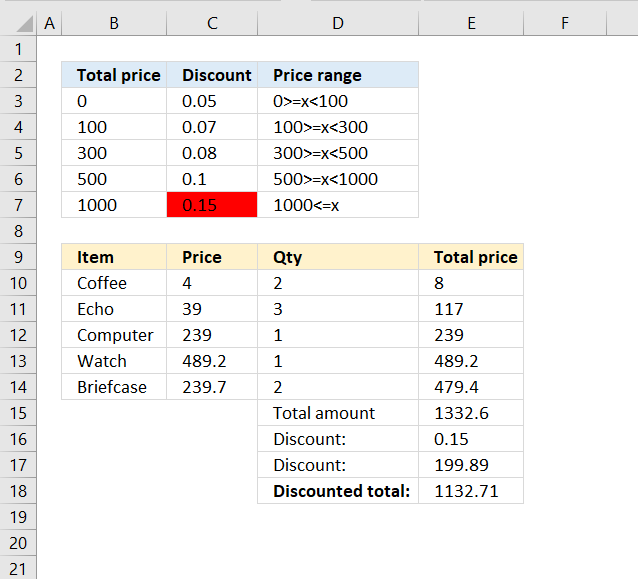
Have you ever tried to build a formula to calculate discounts based on price? The VLOOKUP function is much easier […]
Excel categories
43 Responses to “How to use VLOOKUP/XLOOKUP with multiple conditions”
Leave a Reply
How to comment
How to add a formula to your comment
<code>Insert your formula here.</code>
Convert less than and larger than signs
Use html character entities instead of less than and larger than signs.
< becomes < and > becomes >
How to add VBA code to your comment
[vb 1="vbnet" language=","]
Put your VBA code here.
[/vb]
How to add a picture to your comment:
Upload picture to postimage.org or imgur
Paste image link to your comment.
Hi Oscar,
How do i change the font size and color in a combo box ?
Appreciate your help.
Thanks
Haroun
Haroun,
You can only change font size and color in an active x combo box.
Read more: https://www.ozgrid.com/forum/showthread.php?t=73189
hi oscar,
this above solution is very good and very handy. thank you very much. i made a slight update to this for error-suppression that i thought of sharing here:
={LOOKUP(REPT("Z",25), CHOOSE({1,2},"", INDEX(tbl, SMALL(IF(COUNTIF(search_values, INDEX(tbl, , 1, 1))+COUNTIF(search_values, INDEX(tbl, , 2, 1))+COUNTIF(search_values, INDEX(tbl, , 4, 1)), ROW(tbl)-MIN(ROW(tbl))+1, ""), ROW(A1)), 5)))}
i do not have access to XL'03 in order to check this, but i hope that by _not_ using XL'07-specific "IFERROR" for error-suppression, this formula may be useful for older versions too. am i correct in that assumption?
the purpose for which i employed this formula, i was able to drop the 'area_num' argument from INDEX. is there a specific situation in which *not* having that would wreak havoc?
as always, much thanks and kind regards for all that you share with us.
K. Yantri
i do not have access to XL'03 in order to check this, but i hope that by _not_ using XL'07-specific "IFERROR" for error-suppression, this formula may be useful for older versions too. am i correct in that assumption?
No, use =IF(ISERROR(formula), errorformula, formula)
Thanks for commenting!
Wow I have never thought of using the Table like that...... really potent stuff!
chrisham,
Thank you for commenting! You can use arrays in most excel functions.
I am having a problem getting vlookup to work when asking it to check two different tables based on what data is percent in specific cells. Basically I want it to check one table if a persons gender is male, and another table if the gender is female. Any idea how I can accomplish this? I would really appreciate any help I could get. Thank you very much.
Hi Oscar,
I want to sum up results of Vlookup
please help
For eg,
Product No in Column A and qty sold in Column B
I Will need to derive qty sold of each product. It's a huge data of 2000 odd product list
please suggest
Vicky,
Here is a post about pivot tables:
https://www.get-digital-help.com/analyze-trends-using-pivot-tables/
You can also use formulas. How to extract a unique distinct list:
https://www.get-digital-help.com/how-to-extract-a-unique-list-and-the-duplicates-in-excel-from-one-column/
How to use the sumif function:
https://www.get-digital-help.com/sum-values-between-two-dates-with-criteria-in-excel/
Remove the date criteria.
Hi OScar
SUMIFS,has worked great for me, Thanks for your help. Its been completely Superb
Hi Oscar,
Just a general question, which one is better for huge lookups
Vlookup or Index + Match
can we use index + match instead of vlookup, even if we need to extract values from the right side columns
Thanks
Krishna
Krishna,
Yes, read this: https://exceluser.com/blog/1107/why-index-match-is-far-better-than-vlookup-or-hlookup-in-excel.html
Hi Oscar.. I'm struggling using a lookup formula for extracting values from a large table.. it's something like:
Fruit Market
Apple Walmart
Pear Sigo
Grapes Sigo
Cherry Walmart
Orange 7-eleven
The idea is just extract the fruits from Walmart in a new table but excluding the rest of the fruits.. What do you suggest??? Thanking you in advance for your help...
Jose,
Array formula in cell D2:
=INDEX($A$2:$B$6, SMALL(IF($B$2:$B$6=$D$1, MATCH(ROW($B$2:$B$6), ROW($B$2:$B$6)), ""), ROW(A1)),COLUMN(A1))
Read more:
How to return multiple values using vlookup
Dear Oscar,
I want to vlookup with 2 conditions.
I want to search for value by using two criteria. ex: vlookup with invoice number and serial number search for the discription in other sheet or other related information. Each invoice number has multiple serial numbers or items.Ex. invoice number 1 has 1to 5 items, I need search for all 5 items from database to the main sheet.
Please help
Simao Pereira,
Can you provide some data and the desired outcome?
Does anyone know how to match four columns to pull a single record?
Sheet 1
Description Age Sum of PWK01
Fred A =value reqquired
Mike B =value reqquired
Samuel C =value reqquired
Joshua D =value reqquired
Eric E =value reqquired
Sheet 2
Description Item Age Week 1 Week 2
Fred Kiwis A 31.802571712 37.802571712
Mike Kiwis D 20.528476326 21.528476326
Samuel Kiwis C 52.331048038 51.331048038
Joshua Kiwis F 1457907.9884 1467907.9884
Eric Kiwis E 1481550.2918 1491550.2918
Fred Kiwis B 31.802571712 37.802571712
Mike Kiwis B 20.528476326 21.528476326
Samuel Kiwis G 52.331048038 51.331048038
Joshua Kiwis D 1457907.9884 1467907.9884
Eric Kiwis I 1481550.2918 1491550.2918
Thanks Mike
Mike,
I think I can do that. But I don´t understand your data. What is the desired outcome?
Awesome formula:
=VLOOKUP(C2,IF(B8:B17=C3,A8:E17,""),3,FALSE)
Thanks for sharing this technique.
=VLOOKUP(C2,IF(B8:B17=C3,A8:E17,""),3,FALSE)
Did anyone check this formula ? I get "Value" error (a value used in this formula is of the wrong data type). Any ideas ? ...
Andrei,
It is an array formula.
Select a cell
Type the array formula
Press and hold Ctrl + Shift simultaneously
Press Enter
Release all keys
If you did it right you now have curly brackets before and after the formula, in the formula bar.
It works. I've never done this before. I just feel so silly sometimes - whenever I think I know Excel, something new appears that makes me look like a hairstylist. :(
Dear Oscar Sir,
I am searching for one tricky thing to accomplish using (only) formulas (and not VBA).
I will be thankful if you can help me.
The excel sheet has several columns, I want to filter data by two columns, here, column Speciality = "*Port*", and also, Testing? = "No", now the answer should be value of column "Name" for the first resulting row from the filter formula.
Excel preview data is as follows:
-------------------
Name Speciality Perma? Testng? Success?
A Oil Engine & Automobiles No Yes Yes
B Diamond & Textile Industries No Yes No
C Plastic Industries & Wine No Yes Yes
D IT & Automation No Yes Yes
E Brass Material & Port No Yes Yes
F Port & Shipping Industries No No N/A
G Tours & Spices No Yes Yes
H General No Yes No
I Tours, Divine, Port, etc No No N/A
J Tours & Fisheries No Yes Yes
K Tours & Others No Yes Yes
L Tours & Others Yes Yes Yes
M Film Industries & Hotels Yes Yes No
N Plastic & Other Industries No Yes Yes
O Tours, Wine & Port Yes Yes Yes
Name of person who has speciality matching "PORT" and is not in "Testing" version:
ANSWER = ?? FORMULA ??
Speciality = "*PORT*" + Testing? = "No"
=
[Respective Value of: Column A]
-------------------
In this case, answer should be: F
Awaiting for your reply.
Thanks & Regards,
Deep
Deep,
Array formula in cell A21:
=INDEX($A$2:$A$16, MATCH(1, ISNUMBER(SEARCH(A19, $B$2:$B$16))*($C$2:$C$16=B19), 0))
The answer should be E?
Thanks for the code. I'll check it out. (Sorry for delayed response)
:) Keep up the good work..
Yes sir!! Perfect answer.
Wow! Amazing.. 10 out of 10.. :-)
Hi,
Perhaps you can help me with a similar formula.
I am trying to keep track of components for manufacturing purposes. I have one table where i keep my manufacturing data (product, quantity and date) each of my products require a unique valve and i want to have another table where i can look up the item and if it falls in a particular month indicate the total quantity.
My goal here is to be able to accurately forecast my valve needs.
I have attached an example. https://postimg.org/image/3uvet6l2f/
The incoming valve column i use for valve orders that i place. the cylinder production column is where i need the formula to match the item and time period and return the results.
Thank you very much!
Hi Oscar,
Please how do I handle this case...
An excel column has up to a thousand entries and each entry is to be looked up in another column. The aim is to find out if their is any entry among the up to one thousand entries which is in the other column or not. Since the number of entries to be looked up for is large, I want to avoid doing this one at a time.
Ray,
Use the match function to see if an entry exists in another column.
MATCH(A1,C1:C100000,0) If it returns a number it exists, an error it does not exist.
If we have a data like this in one excel sheet
y 10.94.44.185/
w 10.94.44.184/10.94.44.185/
y 10.94.44.181/10.94.44.182
w 10.94.44.184/10.94.44.185/10.94.44.186
I want Y & W = highest details in second column
Y=10.94.44.181/10.94.44.182
W=10.94.44.184/10.94.44.185/10.94.44.186
which formula can I apply, please let me know some one.
Hi I'm trying to do a vlookup from detail related to a person ID. However, the ID has two records. One record is "Completed" and another record is "Pending Update". How do I formulate it such that the vlookup will pick up the "Pending Update" line instead of the "Completed"
I have a vlookup table that retrieves an employee list.
What I need is when I select an employee from the lookup.
When I move to the next row I only want to be able to select an employee that has not been previously selected.
To add to the above I need the function to select multiple employees.
Hi,
I have a back dated product wise period wise amendments of rates and I want to vlookup the new rate against the product for a specific date in the past.
Oscar, I know this is an older thread, but I am trying to use a version of the VLOOKUP and two conditions (date range)formula, but my table is on another tab and instead of matching my Id's from tab1 to the Ids in table 1,(C2 in the actual formula), it's providing the actual value in my table matching the cell reference from tab 1. So it's giving me the ID in cell A129 instead of trying to find a match for that ID in the table.
I am not sure what I am doing wrong. Can you provide assistance?
Tasha
Can you upload a workbook, I have trouble understanding.
I HAVE BELOW CODE
id name amt
1 Bijankur-BB2 390
2 pkm 240
3 bajra 495
4 induce 535
ORDER is punch in like this 4 Unit Fodder Grass Bijankur-BB2 50 gm Rs. 345
how can i use vlookp & index function
Need Help: I have an file with Column B having entries and i need to match these with my entries in column A. However the column B may have multiple relevant values in column B. How do i do it? Also if i enter any values of column B it has to give me an output of the values i have in column A.
Sample:
S.No City Variable
1 a 123
2 b 111
3 b 124
4 a 145
5 c 167
6 d 192
7 e 122
8 a 111
9 a 109
10 e 110
Type City Here a
S.No City Variable
1 a 123
4 a 145
8 a 111
9 a 109
Hi Srikanth
I believe this article is what you are looking for:Extract multiple records based on a condition
Hi Oscar,
Thanks for the explanation and examples. It helped me in using the conditional within vlookup funtion.
Great help for new learners.
Good Day to you, I have a question.
I need a Vlookup or should it be sumif formulas for 2 sheets, base on two criteria on sheet2. First the date (A1)in sheet 2, then the Item code (B1)in sheet 2, to get the total amount at sheet1 for a certain item.
its kinda like your first graph here, first find the Item, then Region, to get the answer.
but my answer is quantity and need to add up.
hope to get some help from u.
Thanks you so much
Thank you for the examples. I needed a way to look up workers' compensation class code premium rates by state. I had a table of about 200 class codes, in each of 3 states. Being able to find a class code rate based on the state required this 2 column lookup. The IF inside of the VLOOKUP did the trick perfectly!
Dear Sir,
Can you help me with this formula
Project Bid Status Budget Revenue
Sales $203,00 Won $1,000 to $5,000 $5.800,00
Online $151,00 Lost $10,000 to $15,000 $31.700,00
Sales + Online $180,00 Won $5,000 to $10,000 $14.200,00
Online $173,00 Lost $10,000 to $15,000 $9.900,00
Sales $0,00 Won Below $1,000 $16.600,00
Sales + Online $151,00 Won $10,000 to $15,000 $29.400,00
Sales + Online $151,00 Won $1,000 to $5,000 $33.300,00
Online $308,00 Lost Below $1,000 $11.700,00
1. How to make Dropdown list referencing the Bid Amount
2. VLOOKUP formula to display Potential Revenue if we using the dropdown list according to the bid amount above
Thanks