Count cells containing text from list
Table of Contents
- Count cells containing text from list
- Count entries based on date and time
- Count cells with text
- Count specific multiple text strings in a given cell range
- Count identical values if they are on the same row
- Count rows with data
- Count non-empty rows
- Count cells between two values
- Count cells based on a condition and month
- Count cells between specified values
- Count a specific text string in a cell (case sensitive)
- Count text string in a range (case sensitive)
- Count a given pattern in a cell value - overlapping allowed
- Count how many times a string exists in a cell range (case insensitive)
- How to count the number of values separated by a delimiter in a cell?
- How to count the number of values separated by a delimiter in a cell range?
- How to count the number of values separated by a given character?
- How to count the number of values separated by a delimiter - UDF
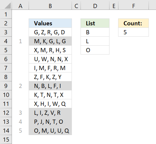
1. Count cells containing text from list
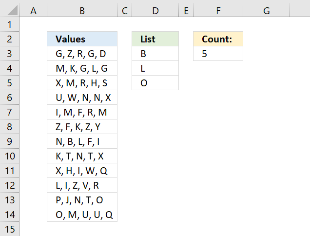
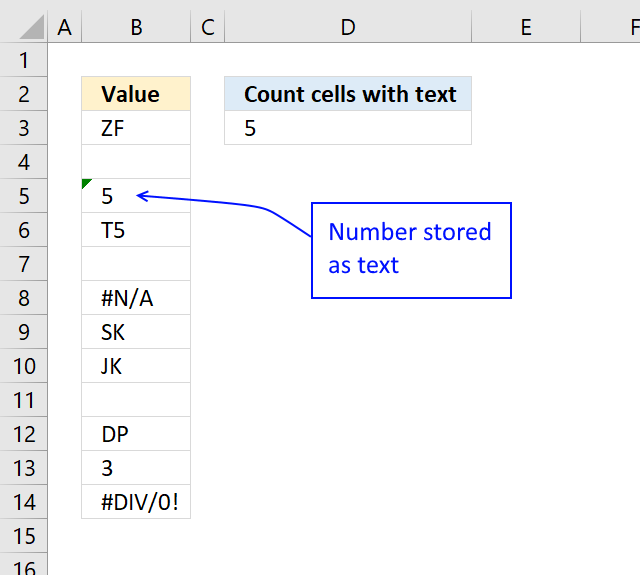
The array formula in cell F3 counts cells in column B that contains at least one of the values in D3:D5. Each cell is only counted once.
To enter the array formula, type the formula in a cell then press and hold CTRL + SHIFT simultaneously, now press Enter once. Release all keys.
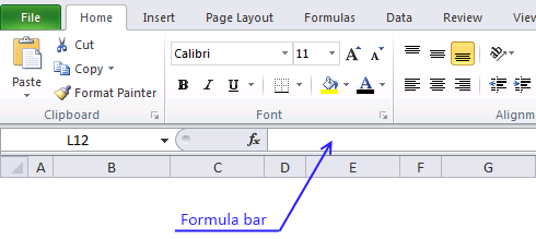
The formula bar now shows the formula with a beginning and ending curly bracket telling you that you entered the formula successfully. Don't enter the curly brackets yourself.
Explaining the formula
The TRANSPOSE function changes the values in D3:D5 from being vertically arranged to being horizontally arranged.
TRANSPOSE(D3:D5)
Note the semicolon and comma characters that separate the values below.
{"B";"L";"O"} => {"B","L","O"}
The SEARCH function requires the values to be arranged in one column in the first argument and in one row in the second argument or vice versa.
That is why the TRANSPOSE function is needed, you could, of course, enter the values horizontally on the worksheet to avoid the TRANSPOSE function.
SEARCH(TRANSPOSE(D3:D5), B3:B14) returns the following array, displayed in the picture below.
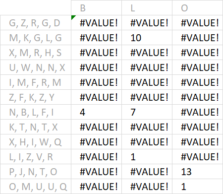
Example, B is found in character position 4 in text string N, B, L, F, I. Note that the SEARCH function returns a #VALUE error if nothing is found.
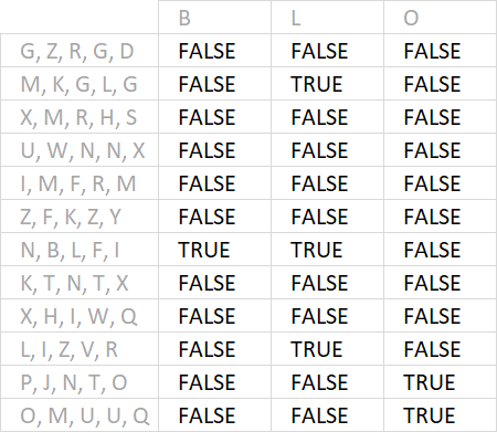
The ISNUMBER function returns TRUE or FALSE determined by a value is a number or not, it happily ignores errors.
ISNUMBER(SEARCH(TRANSPOSE(D3:D5), B3:B14)) returns the following array.
The MMULT function sums the values row by row and returns an array shown in the picture below.
MMULT(ISNUMBER(SEARCH(TRANSPOSE(D3:D5), B3:B14))*1, ROW(D3:D5)^0)
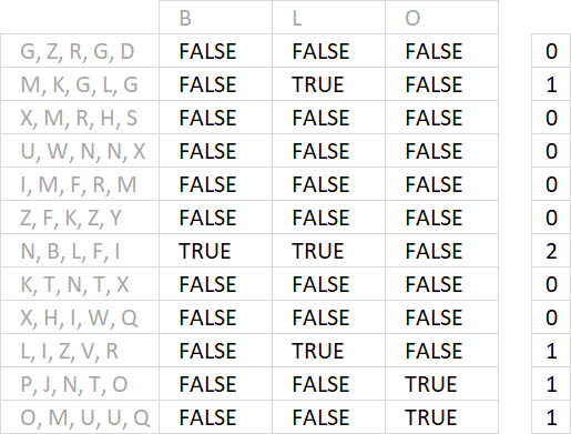
To be able to do that we must use this array as the second argument: {1;1;1} It is determined by the number of cells in the list, in this case, three. They must be 1 and arranged vertically.
That is why I built this formula that builds the array automatically: ROW(D3:D5)^0
The MMULT function can't work with boolean values so I multiply them all by 1 to convert them into 0 (zeros) or 1.
The next thing is to check if the values in the array are larger than 0 (zero).
MMULT(ISNUMBER(SEARCH(TRANSPOSE(D3:D5), B3:B14))*1, ROW(D3:D5)^0)>0
Lastly, the SUM function adds the numbers and returns a total in cell F3.
Get Excel *.xlsx file
Count cells containing text from list.xlsx
Check out this article if you want to count all text strings found in a cell range, in other words, cells might be counted twice or more.
Recommended articles
This article demonstrates an array formula that counts how many times multiple text strings exist in a cell range. The […]
2. Count entries based on date and time
My issue is that I get the date in this format:
7/23/2011 7:00:00 AM
I am trying to count how many entries are between date and time. So I have a shift that starts at 6:30:00 PM and leaves at 7:00:00 AM the next morning. I have tried to convert that to a value to no avail.
I have the cells formatted correctly and tried your other formula =SUM(IF(($A$2:$A$10$D$1),1,0)) + CTRL + SHIFT + ENTER but that returned all records.
I am starting to think that Excel (I'm using 2010) cannot differentiate between the date and time. Any ideas would be greatly appreciated.
Answer:
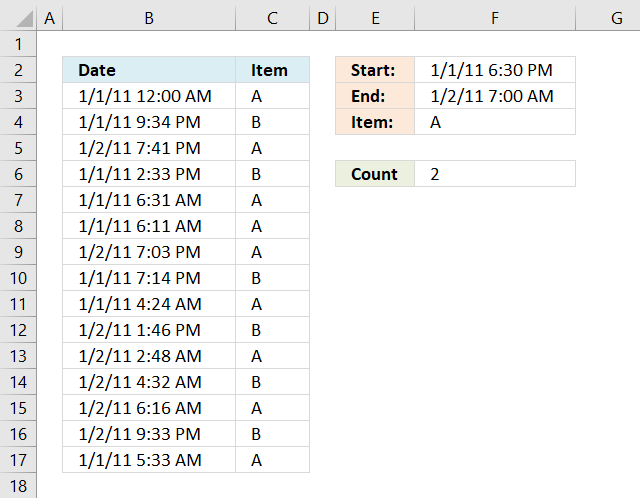
Formula in cell F6:
Explaining formula in cell F6
The COUNTIFS function was introduced in Excel 2007 and it works like the COUNTIF function except you may use multiple conditions at the same time.
COUNTIFS(criteria_range1, criteria1, [criteria_range2, criteria2]…)
| Pair | criteria_range | criteria | Text |
| 1 | B3:B17 | "<="&F3 | Are dates in B3:B17 smaller than end date in cell F3? |
| 2 | B3:B17 | ">="&F2 | Are dates in B3:B17 larger than start date in cell F2? |
| 3 | C3:C17 | F4 | Are Items in c3:C17 equal to cell F4? |
The ampersand character concatenates the logical operators <> and = to each cell or cell range before the COUNTIFS function evaluates the argument. If all conditions return TRUE then the record is counted as 1.
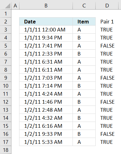
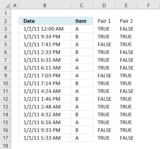
Step 1 - Criteria pair 1
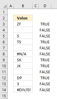
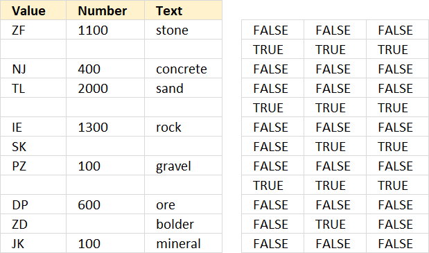
The following image shows in column D date and time entries smaller than or equal to condition in cell F3, TRUE - Smaller, FALSE - larger.
Step 2 - Criteria pair 2
This image shows in column E date and time entries larger than or equal to condition in cell F2, TRUE - Smaller, FALSE - larger.
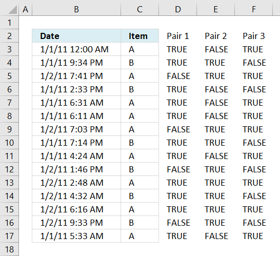
Step 3 - Criteria pair 3
This picture displays in column F items equal to condition in cell F4.
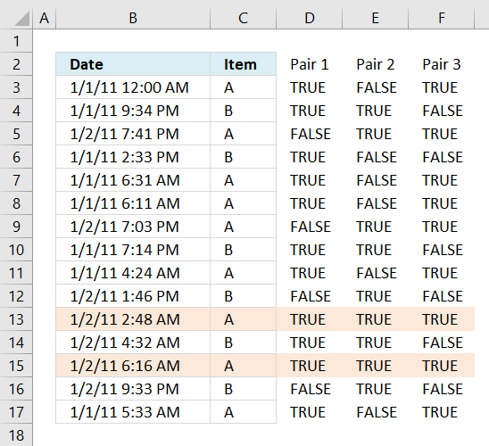
Step 4 - All conditions applied
This image shows which entries meet all conditions. If all conditions evaluate to TRUE then that specific record is counted, the formula returns 2 in cell F6 because two records meet all conditions.
Excel 2003 (and earlier versions) formula in cell F6:
3. Count cells with text
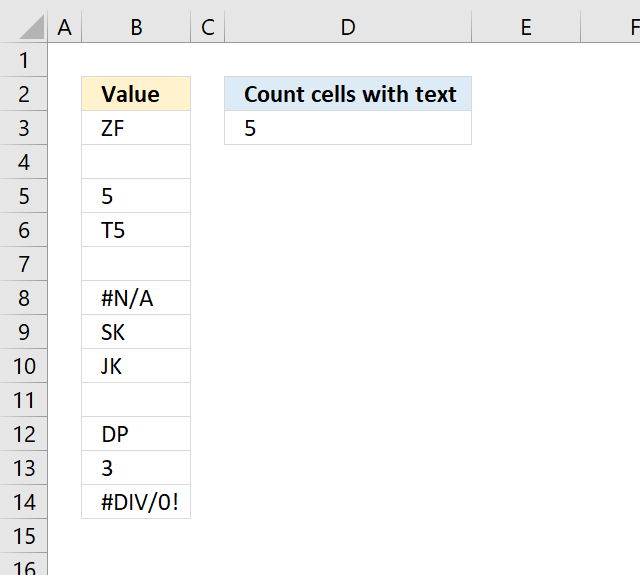
Table of Contents
- Count cells with text
- Count cells with text excluding cells containing a space character
- Count text values returned from an Excel function
- Count text values excluding numbers stored as text
- Get Excel *.xlsx file
3.1. Count cells with text
The following formula in cell D3 counts cells with values stored as text.
In other words, cells containing nothing, errors, boolean values, and numbers are not counted.
Numbers stored as text are counted, as well as cells containing a space a character or more.
3.1.1 Explaining formula
Step 1 - Identify values stored as text
The ISTEXT function returns TRUE or FALSE depending on if a cell has a value stored as text.
ISTEXT(B3:B14)
becomes
ISTEXT({"ZF"; 0; 5; "T5"; 0; #N/A; "SK"; "JK"; 0; "DP"; 3; #DIV/0!})
and returns
{TRUE; FALSE; FALSE ... }.
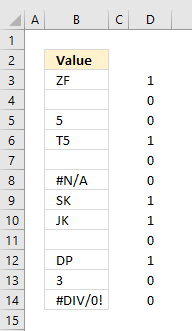
Step 2 - Convert boolean values to numbers
To count boolean values (TRUE, FALSE) we need to convert them into numbers. TRUE = 1 and FALSE = 0 (zero).
ISTEXT(B3:B14)*1
becomes
{TRUE; FALSE; FALSE ... }*1
and returns
{1; 0; 0; ... }.
Step 3 - Count numbers
The SUMPRODUCT function has a great advantage over the SUM function, in most cases, you don't need to enter the formula as an array formula if you are working with arrays.
SUMPRODUCT(ISTEXT(B3:B14)*1)
becomes
SUMPRODUCT({1;0;0;1;0;0;1;1;0;1;0;0})
and returns 5 in cell D3.
1+0+0+1+0+0+1+1+0+1+0+0 = 5.
3.2. Count cells with text excluding cells containing a space character
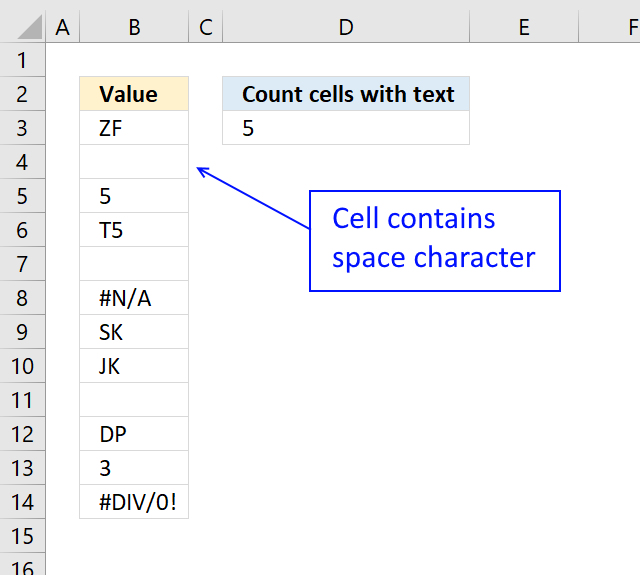
Cell B4 contains a space character, the array formula below does not count cells containing a space character.
B3:B14<>" " makes sure that cells containing a space character are not counted.
3.2.1 How to enter an array formula
To enter an array formula, type the formula in a cell then press and hold CTRL + SHIFT simultaneously, now press Enter once. Release all keys.
The formula bar now shows the formula with a beginning and ending curly bracket telling you that you entered the formula successfully. Don't enter the curly brackets yourself.
3.2.2 Explaining formula
Step 1 - Check if a value is text
The ISTEXT function returns TRUE if argument is text.
Function syntax: ISTEXT(value)
ISTEXT(B3:B14)
becomes
ISTEXT({"ZF"; " "; 5; "T5"; 0; #N/A; "SK"; "JK"; 0; "DP"; 3; #DIV/0!})
and returns
{TRUE; TRUE; FALSE; TRUE; FALSE; FALSE; TRUE; TRUE; FALSE; TRUE; FALSE; FALSE}.
Step 2 - Check if a value is equal to a space character
The less than and greater than characters let you evaluate "not equal to" between two or more values.
B3:B14<>" "
becomes
{"ZF"; " "; 5; "T5"; 0; #N/A; "SK"; "JK"; 0; "DP"; 3; #DIV/0!}<>" "
and returns
{TRUE; FALSE; TRUE; TRUE; TRUE; #N/A; TRUE; TRUE; TRUE; TRUE; TRUE; #DIV/0!}
Step 3 - Replace text values with the result of a logical test
The IF function returns one value if the logical test is TRUE and another value if the logical test is FALSE.
Function syntax: IF(logical_test, [value_if_true], [value_if_false])
IF(ISTEXT(B3:B14),(B3:B14<>" "),0)
becomes
IF({TRUE; TRUE; FALSE; TRUE; FALSE; FALSE; TRUE; TRUE; FALSE; TRUE; FALSE; FALSE},{TRUE; FALSE; TRUE; TRUE; TRUE; #N/A; TRUE; TRUE; TRUE; TRUE; TRUE; #DIV/0!},0)
and returns
{TRUE; FALSE; 0; TRUE; 0; 0; TRUE; TRUE; 0; TRUE; 0; 0}.
Step 4 - Multiply by 1 to convert boolean values to their numerical equivalents
The asterisk character lets you multiply numbers in an Excel formula.
IF(ISTEXT(B3:B14),(B3:B14<>" "),0)*1
becomes
{TRUE; FALSE; 0; TRUE; 0; 0; TRUE; TRUE; 0; TRUE; 0; 0}*1
and returns
{1; 0; 0; 1; 0; 0; 1; 1; 0; 1; 0; 0}.
Step 5 - Add numbers and return a total
The SUM function allows you to add numerical values, the function returns the sum in the cell it is entered in. The SUM function is cleverly designed to ignore text and boolean values, adding only numbers.
Function syntax: SUM(number1, [number2], ...)
SUM(IF(ISTEXT(B3:B14),(B3:B14<>" "),0)*1)
becomes
SUM({1; 0; 0; 1; 0; 0; 1; 1; 0; 1; 0; 0})
and returns 5.
3.3. Count text values returned from an Excel function
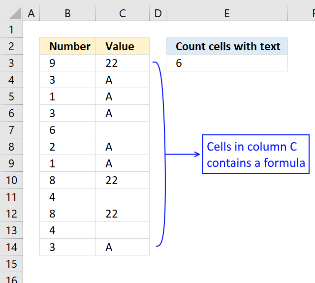
The formula below lets you count text values returned from an Excel function.
The ISTEXT function handles empty values from an Excel function as a text value. To avoid counting those non-values I simply use the smaller than and larger than signs <> meaning not equal to.
3.1 Explaining formula
Step 1 - Check if value is text
The ISTEXT function returns TRUE if argument is text.
Function syntax: ISTEXT(value)
ISTEXT(C3:C14)
becomes
ISTEXT({22; "A"; "A"; "A"; ""; "A"; "A"; 22; ""; 22; ""; "A"})
and returns
{FALSE; TRUE; TRUE; TRUE; TRUE; TRUE; TRUE; FALSE; TRUE; FALSE; TRUE; TRUE}.
Step 2 - Check if a value is not empty
The less than and greater than characters lets you evaluate if a value is "not equal to" another value, the result is a boolean value TRUE or FALSE.
C3:C14<>""
becomes
{22; "A"; "A"; "A"; ""; "A"; "A"; 22; ""; 22; ""; "A"}<>""
and returns
{TRUE; TRUE; TRUE; TRUE; FALSE; TRUE; TRUE; TRUE; FALSE; TRUE; FALSE; TRUE}.
Step 3 - Multiply arrays (AND logic)
ISTEXT(C3:C14)*(C3:C14<>"")
becomes
{FALSE; TRUE; TRUE; TRUE; TRUE; TRUE; TRUE; FALSE; TRUE; FALSE; TRUE; TRUE}*{TRUE; TRUE; TRUE; TRUE; FALSE; TRUE; TRUE; TRUE; FALSE; TRUE; FALSE; TRUE}
and returns
{0; 1; 1; 1; 0; 1; 1; 0; 0; 0; 0; 1}.
Step 4 - Add values and return a total
The SUMPRODUCT function calculates the product of corresponding values and then returns the sum of each multiplication.
Function syntax: SUMPRODUCT(array1, [array2], ...)
SUMPRODUCT(ISTEXT(C3:C14)*(C3:C14<>""))
becomes
SUMPRODUCT({0; 1; 1; 1; 0; 1; 1; 0; 0; 0; 0; 1})
and returns 6.
3.4. Count text values excluding numbers stored as text
This formula counts cells containing text values excluding numbers stored as text from the count.
Cell B5 contains a number stored as text, to exclude that number from the count use the following formula:
3.4.1 Explaining formula
Step 1 - Check if a value is text
The ISTEXT function returns TRUE if argument is text.
Function syntax: ISTEXT(value)
ISTEXT(B3:B14)
becomes
ISTEXT({"ZF";0;"5";"T5";0;#N/A;"SK";"JK";0;"DP";3;#DIV/0!})
and returns
{TRUE; FALSE; TRUE; TRUE; FALSE; FALSE; TRUE; TRUE; FALSE; TRUE; FALSE; FALSE}.
Step 2 - Check if a value is a number
The asterisk character lets you multiply numbers in an Excel formula. It returns a product if both values are numbers and an error if not.
It also converts numbers stored as text like "5" to 5.
B3:B14*1
becomes
{"ZF";0;"5";"T5";0;#N/A;"SK";"JK";0;"DP";3;#DIV/0!}*1
and returns
{#VALUE!; 0; 5; #VALUE!; 0; #N/A; #VALUE!; #VALUE!; 0; #VALUE!; 3; #DIV/0!}.
Step 3 - Check if a value is a number
The ISNUMBER function checks if a value is a number, returns TRUE or FALSE.
Function syntax: ISNUMBER(value)
ISNUMBER(B3:B14*1)
becomes
ISNUMBER({#VALUE!; 0; 5; #VALUE!; 0; #N/A; #VALUE!; #VALUE!; 0; #VALUE!; 3; #DIV/0!})
and returns
{FALSE; TRUE; TRUE; FALSE; TRUE; FALSE; FALSE; FALSE; TRUE; FALSE; TRUE; FALSE}.
Step 4 - Perform boolean opposite
The NOT function returns the boolean opposite to the given argument.
Function syntax: NOT(logical)
NOT(ISNUMBER(B3:B14*1))
becomes
NOT({FALSE; TRUE; TRUE; FALSE; TRUE; FALSE; FALSE; FALSE; TRUE; FALSE; TRUE; FALSE})
and returns
{TRUE; FALSE; FALSE; TRUE; FALSE; TRUE; TRUE; TRUE; FALSE; TRUE; FALSE; TRUE}.
Step 5 - Multiply arrays
The asterisk character lets you also multiply boolean values, this performs AND logic on two arrays. AND logic returns TRUE if both values are TRUE.
TRUE * TRUE = TRUE (1)
TRUE * FALSE = FALSE (0)
FALSE * FALSE = FALSE (0)
The multiplication also converts boolean values to their numerical equivalents.
TRUE - 1
FALSE - 0 (zero)
ISTEXT(B3:B14)*NOT(ISNUMBER(B3:B14*1))
becomes
{TRUE; FALSE; TRUE; TRUE; FALSE; FALSE; TRUE; TRUE; FALSE; TRUE; FALSE; FALSE} * {TRUE; FALSE; FALSE; TRUE; FALSE; TRUE; TRUE; TRUE; FALSE; TRUE; FALSE; TRUE}
and returns
{1; 0; 0; 1; 0; 0; 1; 1; 0; 1; 0; 0}
Step 6 - Add values and return a total
The SUMPRODUCT function calculates the product of corresponding values and then returns the sum of each multiplication.
Function syntax: SUMPRODUCT(array1, [array2], ...)
SUMPRODUCT(ISTEXT(B3:B14)*NOT(ISNUMBER(B3:B14*1)))
becomes
SUMPRODUCT({1; 0; 0; 1; 0; 0; 1; 1; 0; 1; 0; 0})
and returns
5. 1 + 1 + 1 + 1 + 1 = 5
3.5. Get Excel *.xlsx file
4. Count specific multiple text strings in a given cell range
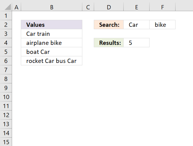
This section demonstrates an array formula that counts how many times multiple text strings exist in a cell range. The formula takes into account if a text string exists multiple times in a single cell, see picture above. Text strings "Car" and "bike" exist 5 times in cell range B3:B6.
Table of contents
- Count specific multiple text strings in a given cell range - case sensitive
- Count specific multiple text strings in a given cell range - case insensitive
4.1. Count specific multiple text strings in a given cell range - case sensitive
It is easy to add more text strings, and adjust cell range E2:F2 in the formula. The following formulas are case-sensitive, however, I will be demonstrating case-insensitive formulas later in this section.
Array formula in cell E4:
or use this slightly larger regular formula:
How to enter an array formula
- Select cell E4.
- Press with left mouse button on in the formula bar.
- Copy above array formula and paste to the formula bar.
- Press and hold CTRL + SHIFT simultaneously.
- Press Enter once.
- Release all keys.
The formula bar displays curly brackets:
Don't enter the curly brackets yourself, they appear automatically.
Explaining array formula in cell D2

Excel has a built-in tool named "Evaluate Formula" tool, it allows you to examine formulas and the calculations they make step by step.
Go to tab "Formulas" on the ribbon, press with left mouse button on "Evaluate Formula" button and a dialog box appears.
Press with left mouse button on the "Evaluate" button on the dialog box to move to the next calculation step, this way you can see all calculation steps a formula does making it easier for you to understand and troubleshoot a formula.
The most important thing to understand in this formula is how arrays can be used.
Step 1 - Count characters in each cell
The LEN function returns a number representing the number of characters in a cell. In this case, the LEN function works with a cell range returning an array of numbers.
Len(B3:B6)
becomes
Len({"Car train"; "airplane bike"; "boat Car"; "rocket Car bus Car"})
and returns {9; 13; 8; 18}.

Step 2 - Replace existing text with the new text string
The SUBSTITUTE function replaces a specific text string in a value, it is case sensitive. The SUBSTITUTE function replaces multiple strings with nothing in this formula.
SUBSTITUTE(text, old_text, new_text, [instance_num])
The old_text argument allows you to use a cell range D1:E1 which is handy in this scenario, note that it returns an array containing eight values.
The first row in the array contains values without the first text string (D1) and the second row contains values without the second text string (E1). This is not a problem as you will see when we go through the remaining steps.
SUBSTITUTE(B3:B6,D1:E1,"")
becomes
SUBSTITUTE({"Car train"; "airplane bike"; "boat Car"; "rocket Car bus Car"},{"Car", "bike"},"")
and returns the following array, see E3:F6 in the image below.

Values in an array are separated by a comma or a semicolon, commas are used between columns and semicolons between rows.
Note, your Excel version may use other characters than commas and semicolons based on the regional settings on your computer.
Step 3 - Count characters in each cell
In this step the LEN function calculates the length of each value in the array after the SUBSTITUTE function has replaced the given text strings.
LEN(SUBSTITUTE(B3:B6, E2:F2, ""))
returns the array displayed in E3:F6 in the image below.

Step 4 - Subtract original character length with substituted values
This step calculates the difference between the number of characters of each value in the array. But the array sizes do not match? The number of horizontal values matches which makes it possible to calculate this arithmetic operation.
LEN(B3:B6)-LEN(SUBSTITUTE(B3:B6,E2:F2,""))
returns the array displayed in E3:F6 in the image below.

Step 5 - Divide with length of each search string
We now know where the given text strings are in the array and also how many they are in each value based on character length. If we divide the length of each value in the array with the numbers of characters in each given text string we can calculate how many times they exist.
(LEN(B3:B6)-LEN(SUBSTITUTE(B3:B6,E2:F2,"")))/LEN(E2:F2)
returns the array displayed in E3:F6 in the image below.

Step 6 - Sum all values
The SUM function adds all numbers in the array.
SUM((LEN(B3:B6)-LEN(SUBSTITUTE(B3:B6,E2:F2,"")))/LEN(E2:F2)
becomes
SUM({1,0;0,1;1,0;2,0})
and returns 5 in cell E4.
4.2. Count specific multiple text strings in a given cell range - case insensitive

The following formulas are not case sensitive in terms of search values, see image above.
Array formula in cell E4:
or use this slightly larger regular formula:
The difference between these formulas and the case-sensitive formulas is the UPPER function. It converts letters to upper case letters.
5. Count identical values if they are on the same row

This article describes a formula that counts values in two columns if they are duplicates on the same row.
What's on this section
- Count identical values if they are on the same row (Array formula)
- Count identical values if they are on the same row (Regular formula)
- Count identical values on the same row comparing values in n columns
- Get Excel file
5.1. Count identical values if they are on the same row (Array formula)
Hi Oscar,Need a formula to count identical numbers in two columns but items must be in same row (position).
12 15
8 8 good count 1
22 19
7 22 for 22 not count cause is not in same row
14 14 good count 2
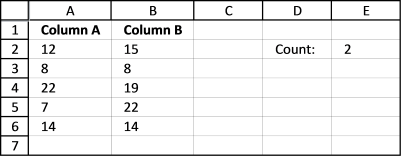
Array formula in cell E2:
5.1.1 How to enter an array formula
- Select cell E2
- Paste the formula in formula bar
- Press and hold CTRL + SHIFT simultaneously
- Press Enter
- Release all keys
Your formula now begins and ends with a curly bracket, if you did it right.
Like this {=SUM((A2:A6=B2:B6)*1)}
Don't enter the curly brackets yourself, they appear automatically.
5.1.2 Explaining formula
Step 1 - Compare values in column A with column B
The equal sign lets you compare value to value, the result is boolean value TRUE if they match (not case-sensitive) and FALSE if they don't.
A2:A6=B2:B6
becomes
{12; 8; 22; 7; 14}={15; 8; 19; 22; 14}
and returns
{FALSE; TRUE; FALSE; FALSE; TRUE}
Step 2 - Multiply boolean values with 1
To be able to sum the values in this array {FALSE; TRUE;FALSE;FALSE;TRUE} we need to convert the boolean values to their numerical equivalents, FALSE = 0 (zero) and TRUE = 1.
(A2:A6=B2:B6)*1
becomes
({FALSE;TRUE;FALSE;FALSE;TRUE})*1
and returns
{0; 1; 0; 0; 1}
Step 3 - Sum values in array
The SUM function adds all numbers in the array and returns a total.
SUM((A2:A6=B2:B6)*1)
becomes
SUM({0; 1; 0; 0; 1})
and returns 2.
5.1.3 Trim space characters
This formula also works with text values, to remove blanks before and after use TRIM function.
5.2. Count identical values if they are on the same row (Regular formula)

5.3. Count identical values on the same row comparing values in n columns

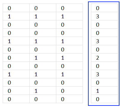
The formula in cell F3 counts the number of rows that contain the same value. In the example shown in the image above row 4, 7, and 9 contain the same value and the formula returns 3.
Note that this formula works with any cell range size, it does not need to be exactly three columns for this formula to work. However, you need to adjust the cell references accordingly in order to get a correct result.
Excel 365 dynamic array formula:
Here is how it works:
- B3:D10=B3:B10: Compare each value on the same row to the first value on the same row. The result is a logic (boolean) array containing TRUE or FALSE.
- AND(a)*1: Perform AND logic to each value on the same row, the result is TRUE or FALSE. Multiply the logical value by 1 to convert the boolean value to it's numerical equivalent.
- BYROW(B3:D10=B3:B10,LAMBDA(a,AND(a)*1)): Perform the calculation per row. This returns an array containing 0 (zero) or 1.
- SUM(BYROW(B3:D10=B3:B10,LAMBDA(a,AND(a)*1))): Add the numbers.
Formula for earlier Excel versions:
5.3.1 Explaining formula
Step 1 - Compare values across columns
The equal sign lets you check if cell values match, the equal sign is a logical operator and returns a boolean (logical) value. TRUE if they match and FALSE if not.
B3:B10=B3:D10
becomes
{12; 8; 22; 7; 14; 5; 7; 11}={12,11,15; 8,8,8; 22,19,22; 7,8,22; 14,14,14; 5,2,6; 7,7,7; 11,18,12}
and returns
{TRUE, FALSE, FALSE;TRUE, TRUE, TRUE;TRUE, FALSE, TRUE;TRUE, FALSE, FALSE;TRUE, TRUE, TRUE;TRUE, FALSE, FALSE;TRUE, TRUE, TRUE;TRUE, FALSE, FALSE}
Step 2 - Convert boolean values
The MMULT function can't handle boolean values, we need to convert TRUE and FALSE to their numerical equivalents. TRUE - 1 and FALSE 0 (zero).
(B3:B10=B3:D10)*1
becomes
{TRUE, FALSE, FALSE;TRUE, TRUE, TRUE;TRUE, FALSE, TRUE;TRUE, FALSE, FALSE;TRUE, TRUE, TRUE;TRUE, FALSE, FALSE;TRUE, TRUE, TRUE;TRUE, FALSE, FALSE}*1
and returns
{1, 0, 0;1, 1, 1;1, 0, 1;1, 0, 0;1, 1, 1;1, 0, 0;1, 1, 1;1, 0, 0}
Step 3 - Calculate column numbers
The COLUMN function calculates the column numbers based on a cell reference.
COLUMN(B3:D10)
returns {2, 3, 4}.
Column B is 2, C is 3 and D is column number 4.
Step 4 - Convert all numbers to number 1
This step converts all column numbers to number 1. This is done by taking each number in the array raised to the 0 (zero) power.
COLUMN(B3:D10)^0
becomes
{2, 3, 4}^0
and returns {1, 1, 1}.
Step 5 - Convert a horizontal range to a vertical range
The TRANSPOSE function allows you to convert a vertical range to a horizontal range, or vice versa.
TRANSPOSE(COLUMN(B3:D10)^0)
becomes
TRANSPOSE({1, 1, 1})
and returns {1; 1; 1}.
The colon and semicolon tell you if an array is arranged vertically or horizontally. This is determined by your computer's regional settings.
Step 6 - Calculate the number of matches per row
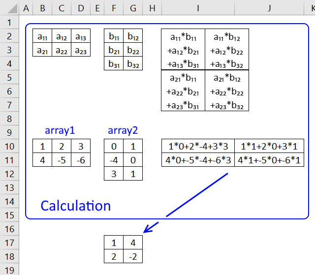
The MMULT function calculates the matrix product of two arrays, an array as the same number of rows as array1 and columns as array2.
MMULT(array1, array2)
MMULT((B3:B10=B3:D10)*1,TRANSPOSE(COLUMN(B3:D10)^0))
becomes
MMULT({1, 0, 0;1, 1, 1;1, 0, 1;1, 0, 0;1, 1, 1;1, 0, 0;1, 1, 1;1, 0, 0}, {1; 1; 1})
and returns {1; 3; 2; 1; 3; 1; 3; 1}.
Step 7 - Check if the number of matches is equal to the number of columns
MMULT((B3:B10=B3:D10)*1,TRANSPOSE(COLUMN(B3:D10)^0))=COLUMNS(B3:D10)
becomes
{1; 3; 2; 1; 3; 1; 3; 1}=3
and returns
{FALSE; TRUE; FALSE; FALSE; TRUE; FALSE; TRUE; FALSE}.
Step 8 - Convert boolean values
The SUMPRODUCT function can't work with boolean values, we need to convert them to their numerical equivalents. TRUE - 1 and FALSE - 0 (zero).
(MMULT((B3:B10=B3:D10)*1,TRANSPOSE(COLUMN(B3:D10)^0))=COLUMNS(B3:D10))*1
becomes
{FALSE; TRUE; FALSE; FALSE; TRUE; FALSE; TRUE; FALSE}*1
and returns {0; 1; 0; 0; 1; 0; 1; 0}.
Step 9 - Add numbers and return total
SUMPRODUCT((MMULT((B3:B10=B3:D10)*1,TRANSPOSE(COLUMN(B3:D10)^0))=COLUMNS(B3:D10))*1)
becomes
SUMPRODUCT({0; 1; 0; 0; 1; 0; 1; 0})
and returns 3.
6. Count rows with data
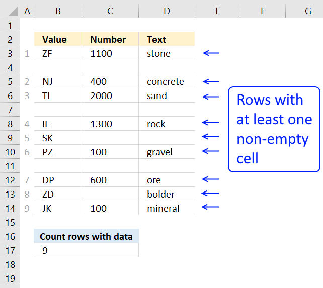
The formula in cell B17 counts rows in cell range B3:D17 when at least one cell per row contains data.
Formula in cell B17:
If your data set, for example, has 5 columns change:
- B3:D14 to your cell range
- the array from {1;1;1} to {1;1;1;1;1}, there must be as many 1's as there a columns in your data set.
- also change <3 to <5
Example, your cell range is A3:G14. The formula becomes:
Explaining formula in cell B17
Step 1 - Check if cell is empty
The equal sign allows you to compare each cell in B3:D14 with an empty value "".
B3:D14="" returns an array of boolean values indicating if a cell is empty or not. {FALSE, FALSE, FALSE; ... }
The picture above shows the array to the right and the corresponding values to the left.
Step 2 - Convert boolean values to numbers
To convert the boolean array to 1 and 0 (zero) I multiply with 1. The parentheses allow you to determine the order of operation.
I want to compare the values with "" before I mutlitply with 1.
(B3:D14="")*1 returns {0, 0, 0; ...)

The picture above shows the array to the right.
Step 3 - Add values row-wise
The MMULT function is great for adding values row by row, however, it can not handle boolean values. The function returns an array of values.
MMULT((B3:D14="")*1,{1;1;1})
There are two arguments in the MMULT function, array1 and array2.
The picture above shows you the result from the MMULT function in the blue rectangle.
To learn more about the MMULT function read this:
Recommended articles
What is the MMULT function? The MMULT function calculates the matrix product of two arrays, an array as the same number […]
Step 4 - Check if each value in the array is smaller than 3.
If there are three empty values in a row that row is empty. That is why I check if each row is less than 3 indicating that at least one cell is not empty.
MMULT((B3:D14="")*1,{1;1;1})<3 returns {TRUE; FALSE; TRUE; TRUE; FALSE; TRUE; TRUE; TRUE; FALSE; TRUE; TRUE; TRUE}
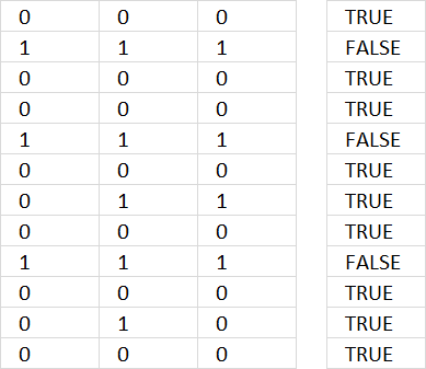
The array is shown to the right in the picture above.
Step 5 - Count rows
To be able to sum the array of boolean values I have to multiply with 1 to convert them to 1 or 0 (zero). TRUE = 1 and FALSE = 0.
SUMPRODUCT((MMULT((A3:G14="")*1,{1;1;1;1;1;1;1})<7)*1)
becomes
SUMPRODUCT({TRUE; FALSE; TRUE; TRUE; FALSE; TRUE; TRUE; TRUE; FALSE; TRUE; TRUE; TRUE}*1)
becomes
SUMPRODUCT({TRUE; FALSE; TRUE; TRUE; FALSE; TRUE; TRUE; TRUE; FALSE; TRUE; TRUE; TRUE}*1)
becomes
SUMPRODUCT({1; 0; 1; 1; 0; 1; 1; 1; 0; 1; 1; 1}) and returns 9 in cell B17.
Why not use the SUM function? Then you would have to enter the formula as an array formula.
Get Excel *.xlsx file
7. Count complete rows
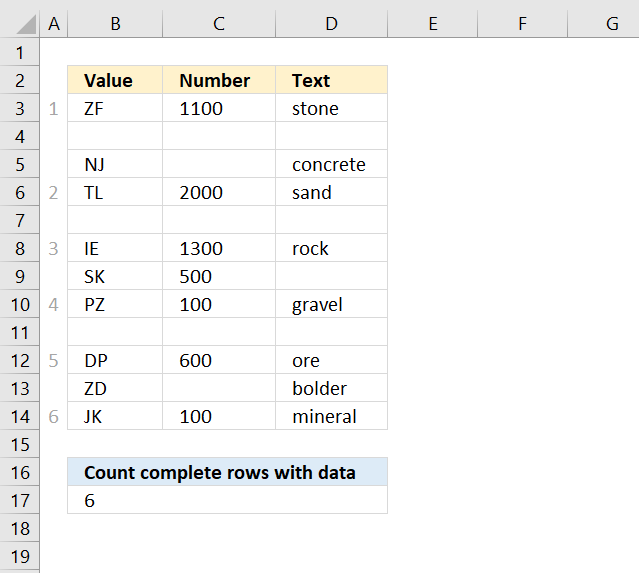
The following formula in cell B17 counts complete rows, in other words, all cells in a row must be non-empty.
See formula in picture above.
8. Count cells between two values
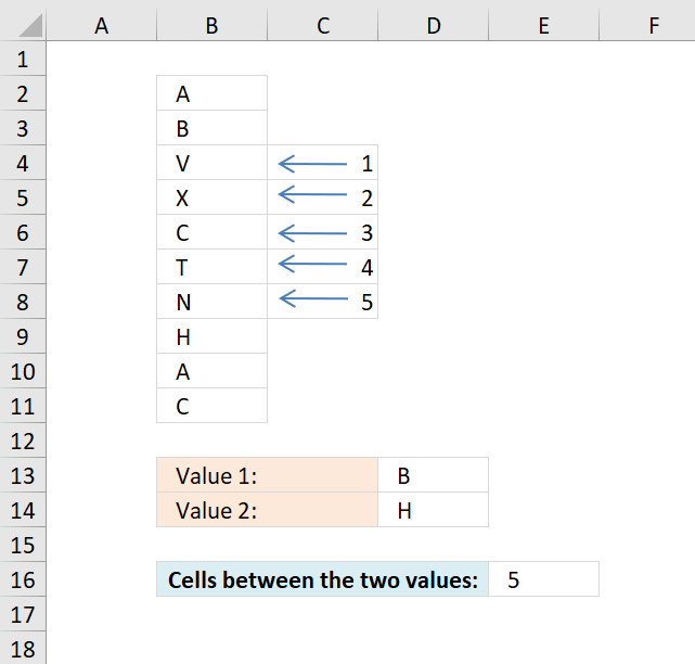
The formula in cell E16 counts the number of cells between value B and H, Value B is in cell B3 and H is in B9, cells B4, B5, B6, B7 and B8 are in between.
Explaining formula in cell E16
Step 1 - Find value in cell D13 in cell range B2:B11
The MATCH function finds the relative position of a value in an array or cell range.
MATCH(D13, B2:B11, 0)
becomes
MATCH("B", {"A"; "B"; "V"; "X"; "C"; "T"; "N"; "H"; "A"; "C"}, 0)
and returns 2.
Step 2 - Find value in cell D14 in cell range B2:B11
MATCH(D14, B2:B11, 0)
becomes
MATCH("H", {"A"; "B"; "V"; "X"; "C"; "T"; "N"; "H"; "A"; "C"}, 0)
and returns 8.
Step 3 - Subtract positions
MATCH(D13, B2:B11, 0)-MATCH(D14, B2:B11, 0)
becomes
2-8 equals -6.
Step 4 - Remove sign
We don't know where the values are in the cell range so it may happen that we get a negative number from time to time, this example is such occasion. The ABS function removes the sign from a number.
ABS(MATCH(D13, B2:B11, 0)-MATCH(D14, B2:B11, 0))
becomes
ABS(-6)
and returns 6.
Step 5 - Subtract with 1
The calculation counts the last cell as well, we only need the cells in between.
ABS(MATCH(D13, B2:B11, 0)-MATCH(D14, B2:B11, 0))-1
becomes
6-1
and returns 5 in cell E16.
Get Excel *.xlsx file
formula to count cells between two values.xlsx
9. Count cells based on a condition and month
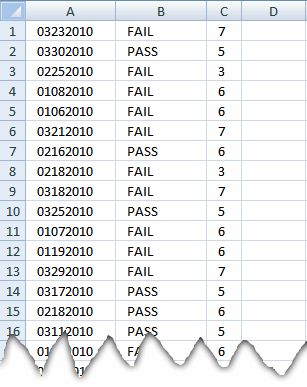
In A column, there are dates in mmddyyy format and in B column, there are two variables uses either "PASS" or "FIAIL". All I want to do is to count the "PASS" in individual month range.
Can someone help me in it. I am able to count days of month from the column A but can not link it with Column B.
Answer:
Formula in cell C1:
Copy cell C1 and paste down as far as needed.
Explaining formula in cell C1
Step 1 - Create arrays
The YEAR function returns the year from an Excel date.
=SUMPRODUCT(--(YEAR(A1)=YEAR($A$1:$A$30)), --(MONTH(A1)=MONTH($A$1:$A$30)), --(B1=$B$1:$B$30))
contains three criteria. The first criterion: --(YEAR(A1)=YEAR($A$1:$A$30))
becomes
--(2010=2010, 2010, 2010, 2010, 2010, 2010, 2010, 2010, 2010, 2010, 2010, 2010, 2010, 2010, 2010, 2010, 2010, 2010, 2010, 2010, 2010, 2010, 2010, 2010, 2010, 2010, 2010, 2010, 2010, 2010)
becomes
--(TRUE, TRUE, TRUE, TRUE, TRUE, TRUE, TRUE, TRUE, TRUE, TRUE, TRUE, TRUE, TRUE, TRUE, TRUE, TRUE, TRUE, TRUE, TRUE, TRUE, TRUE, TRUE, TRUE, TRUE, TRUE, TRUE, TRUE, TRUE, TRUE, TRUE)
and creates this array: (1, 1, 1, 1, 1, 1, 1, 1, 1, 1, 1, 1, 1, 1, 1, 1, 1, 1, 1, 1, 1, 1, 1, 1, 1, 1, 1, 1, 1, 1)
The MONTH function returns a number from 1 to 12 representing the month. Jan = 1, Feb = 2 ... Dec = 12.
The second criterion: --(MONTH(A1)=MONTH($A$1:$A$30))
creates this array: (1, 1, 0, 0, 0, 1, 0, 0, 1, 1, 0, 0, 1, 1, 0, 1, 0, 0, 0, 0, 0, 1, 0, 0, 1, 1, 0, 1, 0, 0)
The third criterion: --(B1=$B$1:$B$30)
creates this array: (1, 0, 1, 1, 1, 1, 0, 1, 1, 0, 1, 1, 1, 0, 0, 0, 1, 0, 0, 0, 0, 1, 1, 0, 1, 0, 0, 1, 0, 1)
Step 2 - The product of three arrays
The SUMPRODUCT function multiplies the arrays (product) and then add the numbers in the array and returns a total (sum).
The entire formula now becomes
=SUMPRODUCT((1, 1, 1, 1, 1, 1, 1, 1, 1, 1, 1, 1, 1, 1, 1, 1, 1, 1, 1, 1, 1, 1, 1, 1, 1, 1, 1, 1, 1, 1), (1, 1, 0, 0, 0, 1, 0, 0, 1, 1, 0, 0, 1, 1, 0, 1, 0, 0, 0, 0, 0, 1, 0, 0, 1, 1, 0, 1, 0, 0), (1, 0, 1, 1, 1, 1, 0, 1, 1, 0, 1, 1, 1, 0, 0, 0, 1, 0, 0, 0, 0, 1, 1, 0, 1, 0, 0, 1, 0, 1))
and then
=SUMPRODUCT((1, 1, 1, 1, 1, 1, 1, 1, 1, 1, 1, 1, 1, 1, 1, 1, 1, 1, 1, 1, 1, 1, 1, 1, 1, 1, 1, 1, 1, 1)*(1, 1, 0, 0, 0, 1, 0, 0, 1, 1, 0, 0, 1, 1, 0, 1, 0, 0, 0, 0, 0, 1, 0, 0, 1, 1, 0, 1, 0, 0)*(1, 0, 1, 1, 1, 1, 0, 1, 1, 0, 1, 1, 1, 0, 0, 0, 1, 0, 0, 0, 0, 1, 1, 0, 1, 0, 0, 1, 0, 1))
becomes
Step 3 - Sum array
=SUMPRODUCT(1, 0, 0, 0, 0, 1, 0, 0, 1, 0, 0, 0, 1, 0, 0, 0, 0, 0, 0, 0, 0, 1, 0, 0, 1, 0, 0, 1, 0, 0) equals 7.
Picture of formula calculations in cell C5
In order to show headers I had to adjust formula ranges:

10. Count cells between specified values
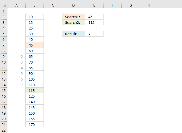
This article demonstrates formulas that calculate the number of cells between two values, the first scenario involves two search values and unique numbers in column B.
If this is not what you are looking for then scroll down to see more examples.
Formula in cell E5:
Since there is only one instance of each search value in column B you only need a small formula to calculate the number of cells between the values.
Column A shows the cell count between the two values.
Explaining formula in cell E5
The formula finds the first value specified in cell E2 (45) in column B and returns the relative position of 45. It then continues with the second value given in cell E3.
The difference between the calculated relative positions is the number of cells between the values.
Step 1 - Find position of first value
The MATCH function returns the relative position of the value in cell E2 in cell range B2:B21.
MATCH(E2,$B$2:$B$21,0)
returns 6. Value 45 is the sixth value in the array.
Step 2 - Find position of second value
MATCH(E3,$B$2:$B$21,0)
returns 14. Value 115 is the 14th value in the array.
Step 3 - Subtract row numbers
MATCH(E2,$B$2:$B$21,0)-MATCH(E3,$B$2:$B$21,0)
becomes
6-14
and returns -8.
Step 4 - Remove sign
The ABS function converts negative numbers to positive numbers.
ABS(MATCH(E2,$B$2:$B$21,0)-MATCH(E3,$B$2:$B$21,0))-1
becomes
ABS(-8)-1
becomes
8-1 and returns 7 in cell E5.
10.1 Multiple values - two search values
The image above shows the second scenario, there are multiple instances of each search value in column B. This requires a somewhat more complicated formula to get the smallest number of cells between the two search values.
The order makes no difference, in other words, if search value 2 is found first makes no difference in this calculation.
Array formula in cell E5:
To enter an array formula, type the formula in a cell then press and hold CTRL + SHIFT simultaneously, now press Enter once. Release all keys.
The formula bar now shows the formula with a beginning and ending curly bracket telling you that you entered the formula successfully. Don't enter the curly brackets yourself.
Explaining formula in cell E5
Step 1 - Calculate row numbers for first search value
The IF function has three arguments, the first one must be a logical expression. If the expression evaluates to TRUE then one thing happens (argument 2) and if FALSE another thing happens (argument 3).
IF(B2:B25=E2, ROW(B2:B25), "")
returns {""; ""; ... ; 25}.
Step 2 - Calculate row numbers for second search value
The TRANSPOSE function rearranges values distributed vertically to horizontally.
TRANSPOSE(IF(B2:B25=E3, ROW(B2:B25), ""))
returns {"", "", ... , ""}.
Step 3 - Subtract first array with second array
IF(B2:B25=E2, ROW(B2:B25), "")-TRANSPOSE(IF(B2:B25=E3, ROW(B2:B25), ""))
returns an array too big to show here, however, an image would work if I replace all error values with a "-".
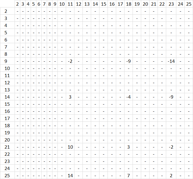
What does the image above tell us? It shows row numbers horizontally and vertically. The first search value (1) has its row numbers displayed vertically, there are four instances of the search value in column B, row 9, 14, 21 and 25.
The second search value har its row numbers displayed horizontally, it is found on row 11, 18 and 23. Example, the intersection of 9 and 11 shows -2. It means that 9-11 equals -2, the whole array shows the intersection between all instances of each search value.
This allows us to extract the smallest distance between two cells, or if you like the largest distance or any in between.
Step 4 - Convert negative values to positive values
The ABS function removes the minus sign from negative values.
ABS(IF(B2:B25=E2, ROW(B2:B25), "")-TRANSPOSE(IF(B2:B25=E3, ROW(B2:B25), "")))

Step 5 - Extract smallest number
The AGGREGATE function is better than the SMALL function, it also lets you ignore error values.
AGGREGATE(15, 6, ABS(IF(B2:B25=E2, ROW(B2:B25), "")-TRANSPOSE(IF(B2:B25=E3, ROW(B2:B25), ""))), 1)-1
becomes
2-1
and returns 1 in cell E5.
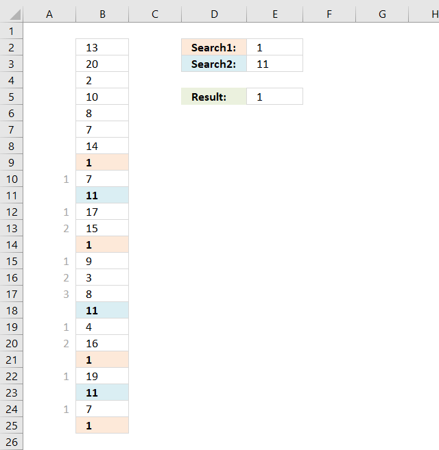
10.2 Multiple values - one search value
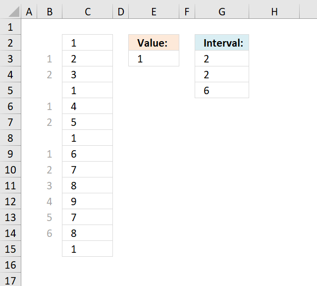
I need to count in a list the interval between the same value.
Example list,
1-2-3-1-4-5-1-6-7-8-9-7-8-1
So the answer must be for the value 1 the spaces are 2,2,6.
thank you
Answer:
Array Formula in cell E2:
How to create an array formula
- Select cell E2
- Type above array formula
- Press and hold Ctrl + Shift
- Press Enter once
- Release all keys
How to copy array formula
- Select cell E2
- Copy (Ctrl + c)
- Select cell range E3:E5
- Paste (Ctrl + v)
Explaining formula in cell E2
There are two parts that calculate the position of the first instance and the second instance, the formula then subtracts the positions in order to get the distance.
Step 1 - Get position of second instance
SMALL(IF($C$2:$C$15=$E$3, MATCH(ROW($C$2:$C$15), ROW($C$2:$C$15)), ""), ROW(A1)+1)
becomes SMALL({1;"";"";4;"";"";7;"";"";"";"";"";"";14},2)
and returns 4. The second instance of 1 is found on row 4 (C5 is on row 4 in cell range $C$2:$C$15).
Step 2 - Get position of first instance
SMALL(IF($C$2:$C$15=$E$3, MATCH(ROW($C$2:$C$15), ROW($C$2:$C$15)), ""), ROW(A1))
becomes SMALL({1;"";"";4;"";"";7;"";"";"";"";"";"";14}, 1)
and returns 1. The first instance of 1 is found on row 1 (C2 is on row 1 in cell range $C$2:$C$15).
Step 3 - Subtract positions
SMALL(IF($C$2:$C$15=$E$3, MATCH(ROW($C$2:$C$15), ROW($C$2:$C$15)), ""), ROW(A1)+1)-SMALL(IF($C$2:$C$15=$E$3, MATCH(ROW($C$2:$C$15), ROW($C$2:$C$15)), ""), ROW(A1))-1
becomes
4-1-1
and returns 2 in cell G3.
How to remove #num errors
11. Count a specific text string in a cell
Question: How do I count how many times a text string exists in a cell value in Excel?
Answer:
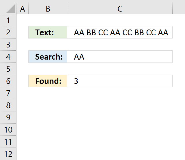
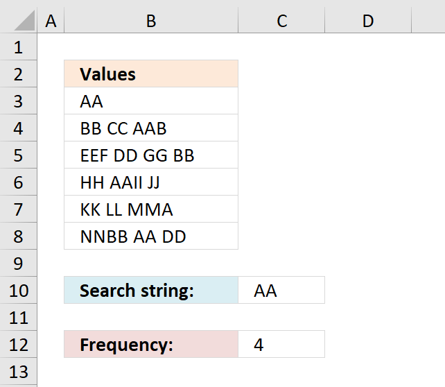
The formula in cell C6 counts how many times a given text string is found in a cell value. The count is case sensitive meaning AA counts AA but not lower case aa, or aA etc.
Formula in C6:
11.1 Explaining formula in cell C6
Step 1 - Substitute given text string with nothing
SUBSTITUTE(C2, C4, "")
returns " BB CC CC BB CC ".
Step 2 - Count text string characters
LEN(SUBSTITUTE(C2, C4, ""))
becomes
LEN(" BB CC CC BB CC ")
and returns 17.
Step 3 - Count text string characters in cell C2
LEN(C2)
becomes
LEN("AA BB CC AA CC BB CC AA")
and returns 23.
Step 4 - Subtract original character length with new text string character length
LEN(C2)-LEN(SUBSTITUTE(C2, C4, ""))
becomes
23 - 17
and returns 6.
Step 5 - Divide with search string character length
(LEN(C2)-LEN(SUBSTITUTE(C2, C4, "")))/LEN(C4)
becomes
6/LEN(C4)
becomes
6/2
and returns 3 in cell C6.
11.2 Get Excel *.xlsx file
Count specific text string in a cell.xlsx
12. Count text string in a cell range (case sensitive)
Question:
How do I count the number of times a text string exists in a column? The text string may exist multiple times in a cell, each instance is counted.
Answer:

Array formula in cell B11:
12.1 How to create an array formula
- Copy array formula (Ctrl + c)
- Select cell B11
- Paste array formula (Ctrl + v) to formula bar
- Press and hold Ctrl + Shift
- Press Enter
- Release all keys
You can also use this formula to count how many times a specific character exists in a column in excel.
12.2 Explain array formula in cell B11
=(SUM(LEN(tbl))-SUM(LEN(SUBSTITUTE(tbl, $B$9, ""))))/LEN($B$9)
Step 1 - Replace existing text strings with new text string in named range tbl (A1:A6)
Substitute(text, old_text, new_text, [instance_num]) replaces existing text with new text in a text string
SUBSTITUTE(tbl, $B$9, "")
returns this array: {"";"BB CC B";... ;"NNBB DD"}
Step 2 - Return the number of characters in the named range tbl (A1:A6) without text string "AA"
SUM(LEN(SUBSTITUTE(tbl, $B$9, "")))
and returns 44
Step 3 - Return the number of characters in the named range tbl (A1:A6)
SUM(LEN(A1:A6))
becomes
SUM({2;9;12;10;9;10})
returns 52.
Step 4 - Return the number of characters in cell B9
(SUM(LEN(A1:A6))-SUM(LEN(SUBSTITUTE(A1:A6, $B$9, ""))))/LEN($B$9)
LEN($B$9)
becomes
LEN("AA")
returns 2.
Step 5 - All together
(SUM(LEN(A1:A6))-SUM(LEN(SUBSTITUTE(A1:A6, $B$9, ""))))/LEN($B$9)
becomes (52-44)/2) becomes 8/2 and returns 4.
2.3 Get Excel file
count-text-string-in-a-column.xls
13. Count a given pattern in a cell value - overlapping allowed
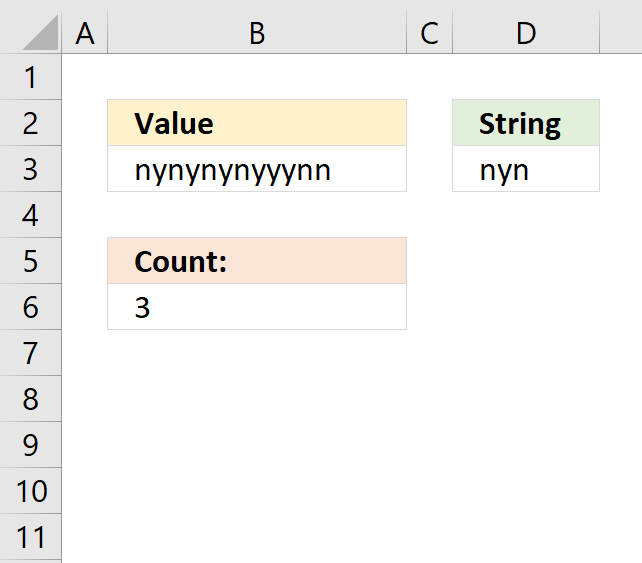
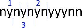
The formula in cell B6 counts how many times the string (D3) is found in a cell value (B3) even if it overlaps another match.
Formula in cell B6:
A regular count would result in 2 matches, see picture below.
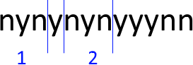
A count where overlapping is allowed returns 3 matches and this is what is demonstrated in this article.
3.1 Explaining formula in cell B6
Step 1 - Build an array from 1 to the number of characters in the cell value
The LEN function counts the number of characters in cell B3.
LEN(B3) returns 13.
The INDEX function returns a cell reference based on a row number.
ROW(A1:INDEX(A1:A1000, LEN(B3)))
becomes
ROW(A1:INDEX(A1:A1000, 13))
becomes
ROW(A1:A13) and returns {1; 2; ... ; 13}
The ROW function returns the row number of a cell. If a cell range is used the ROW function returns an array of row numbers.
Step 2 - Extract all possible substrings from cell value
MID(B3, ROW(A1:INDEX(A1:A1000, LEN(B3))), LEN(D3))
returns the following array:
Step 3 - Check if substring is equal to search string
MID(B3, ROW(A1:INDEX(A1:A1000, LEN(B3))), LEN(D3))=D3
returns {TRUE; FALSE; ... ; FALSE}.
Step 4 - Convert boolean values to the corresponding number
The SUMPRODUCT function can't handle boolean values so the SIGN function converts them into numbers. TRUE = 1 and FALSE = 0.
SIGN(MID(B3, ROW(A1:INDEX(A1:A1000, LEN(B3))), LEN(D3))=D3)
returns {1; 0; 1; ... ; 0}.
Step 5 - Count values in array
SUMPRODUCT(SIGN(MID(B3, ROW(A1:INDEX(A1:A1000, LEN(B3))), LEN(D3))=D3))
becomes SUMPRODUCT({1; 0; 1; 0; 1; 0; 0; 0; 0; 0; 0; 0; 0})
and returns 3 in cell B6. 1 + 0 + 1 + 0 + 1 + 0 + 0 + 0 + 0 + 0 + 0 + 0 + 0 = 3.
13.2 Get Excel *.xlsx file
Count overlapping text string in a cell.xlsx
14. Count how many times a string exists in a cell range (case insensitive)
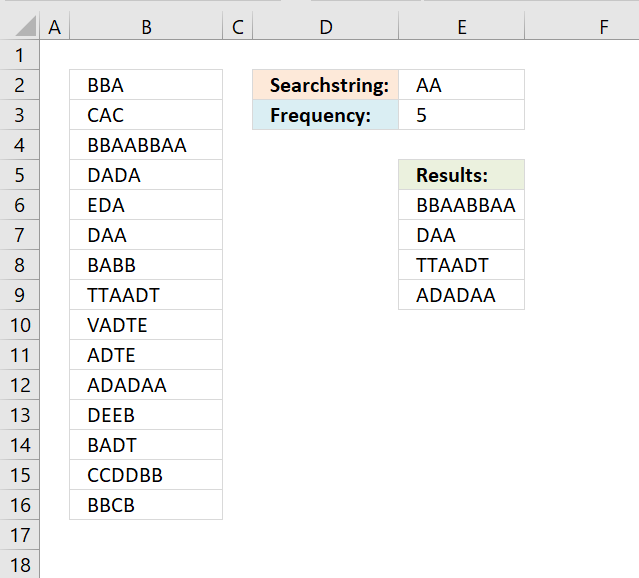
Question: How do I count how many times a word exists in a range of cells? It does not have to be an exact match but case sensitive. Column A1:A15 is the cell range.
Answer:
Cell E2 is the search string. In cell E3 an array formula counts the number of times the search string is found in cell range A1:A15.
Case sensitive formula in cell E3:
Explaining formula in cell E3
Step 1 - Count characters in each cell
The LEN function counts characters in a cell.
LEN(B2:B16)
returns {3;3;8;4;3;3;4;6;5;4;6;4;4;6;4}
Step 2 - Substitue search string with nothing in all cells
The SUBSTITUTE function lets you replace a text string with another text string in a cell value or cell range.
SUBSTITUTE($B$2:$B$16, $E$2, "")
returns {"BBA";"CAC";... ;"BBCB"}
Step 3 - Count characters in array
LEN(SUBSTITUTE($B$2:$B$16, $E$2, ""))
returns {3;3;... ;4}
Step 4 - Subtract arrays
LEN(B2:B16)-LEN(SUBSTITUTE($B$2:$B$16, $E$2, ""))
returns {0;0;4;... ;0}
Step 5 - Divide with cell length
(LEN(B2:B16)-LEN(SUBSTITUTE($B$2:$B$16, $E$2, "")))/LEN($E$2
returns {0;0;0.5;...;0}
Step 6 - Sum number sin array
The SUMPRODUCT is better in this case because you are not required to enter the formula as an array formula to do the calculations.
SUMPRODUCT((LEN(B2:B16)-LEN(SUBSTITUTE($B$2:$B$16, $E$2, "")))/LEN($E$2))
returns 5 in cell E2.
Case insensitive formula in cell E3:
Array formula in cell E6:
Get *.xlsx file
string exist in multiple cells.xlsx
15. How to count comma-separated values in a cell?

The following formula counts the number of strings in a single cell using a comma as a delimiting character.
Formula in cell C3:
Explaining formula in cell C3
Step 1 - Substitute comma with nothing
The SUBSTITUTE function replaces a specific text string in a value.
SUBSTITUTE(text, old_text, new_text, [instance_num])
SUBSTITUTE(B3,",","") returns "aaEE gg".
Step 2 - Count characters in the substituted text
The LEN function counts the number of characters in a string.
LEN(SUBSTITUTE(B3,",","")) returns 8.
Step 3 - Count characters in the original text
LEN(B3) returns 10.
Step 4 - Subtract original text length with substituted text length
LEN(B3)-LEN(SUBSTITUTE(B3,",",""))+1 becomes 10-8+1 equals 3.
16. How to count comma-separated values in a cell range?

Array formula in cell C3:
How to enter an array formula
Enter the formula as a regular formula if you use Excel 365, follow these steps if you use an older version.
- Copy above formula.
- Double press with left mouse button on cell C3.
- Paste to cell C3
- Press and hold CTRL + SHIFT keys simultaneously.
- Press Enter once.
- Release all keys.
The formula will now look like this: {=SUM(LEN(B3:B8)-LEN(SUBSTITUTE(B3:B8, ",", ""))+1)}
Don't enter these characters yourself, they appear automatically.
Explaining formula in cell C3
Step 1 - Substitute comma with nothing
The SUBSTITUTE function replaces a specific text string in a value.
SUBSTITUTE(text, old_text, new_text, [instance_num])
SUBSTITUTE(B3:B8, ",", "") returns {"aaEE gg";"jjoopp";"uuff bb";"uu";"xC Oy";"z OY RTEDSW"}.
Step 2 - Count characters in the substituted text
The LEN function counts the number of characters in a string.
LEN(SUBSTITUTE(B3:B8, ",", "")) returns {8; 6; 7; 2; 5; 11}.
Step 3 - Count characters in the original text
LEN(B3:B8) returns {10; 8; 9; 2; 6; 14}.
Step 4 - Subtract original text length with substituted text length
LEN(B3)-LEN(SUBSTITUTE(B3,",",""))+1 returns {3; 3; 3; 1; 2; 4}.
17. How to count character-separated values in a cell?

The formula in cell C3 uses the characters given in cell E3 to separate and count values in B3. Cell E3 contains " | ", however, you can use whatever characters you want. For example, you can use this formula to separate and count values using a blank as a delimiting character.
Formula in cell C3:
18. How to count the number of values separated by a delimiter - UDF

I received an email from one of my seven blog readers (joke).
In Excel, I have a column, say A, with some cells blank and some cells with text.
In another column, say B, each *cell* contains many words, separated by a comma.
For every cell in B, I need to check to see how many of the words from column A are in the cell and output the total count of matches.
I built a user-defined function for this, if you have a regular formula you think can solve this, please share. This animated picture explains it all.
The formula in cell C2 is a user defined function. You build a UDF just like a macro using the Visual Basic Editor (VBA).
The first argument (B2) in this custom made function is a cell reference to comma-separated values, in a single cell. The second argument ($A$2:$A$20) is a reference to cell range that you want to count, make sure it is a single column cell reference.
18.1 User-defined function VBA code
Function CountWords(a As String, b As Range)
Dim Words() As String
Dim Value As Variant, cell As Variant
Dim c As Single
Words = Split(a, ",")
For Each Value In Words
    For Each cell In b
        If UCase(WorksheetFunction.Trim(cell)) = UCase(WorksheetFunction.Trim(Value)) Then c = c + 1
    Next cell
Next Value
CountWords = c
End Function
18.2 Where to put the VBA code?
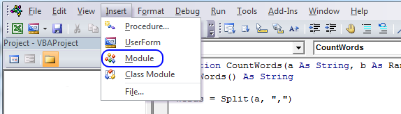
To build a user-defined function, follow these steps:
- Press Alt + F11 to open the visual basic editor.
- Press with left mouse button on "Insert" on the top menu.
- Press with left mouse button on "Module", see the image above.
- Copy the VBA code above and paste it to the code module.
- Return to Excel.
18.3 Explaining the user-defined function
Function name and arguments
A user defined function procedure always start with "Function" and then a name. This udf has two arguments, a and b. Variable a is a string and b is a range.
Function CountWords(a As String, b As Range)
Declaring variables
Dim Words() As String
Dim Value As Variant, cell As Variant
Dim c As Single
Words() is a dynamic string array. Value and cell are variants. c is a single data type. Read more about Defining data types.
Split function
Words = Split(a, ",")
The Split function accepts a text string and returns a zero-based, one-dimensional array containing all sub strings. Split allows you also to specify a delimiting character, default is the space character.
For ... Next statement
For Each Value In Words
...
Next Value
Repeats a group of statements a specified number of times. In this case as many times as there are values in the array Words.
If function
If UCase(WorksheetFunction.Trim(cell)) = UCase(WorksheetFunction.Trim(Value)) Then c = c + 1
The Ucase function converts a string to uppercase letters. The WorksheetFunction.Trim method removes all spaces from text except for single spaces between words.
The If function compares cell and Value and if they match 1 is added to c.
The udf returns...
CountWords = c
The udf returns the value in c.
End a udf
End Function
A function procedure ends with the "End function" statement.
Count category
Count values category
This article describes how to count unique distinct values. What are unique distinct values? They are all values but duplicates are […]
This article explains how to count cells highlighted with Conditional Formatting (CF). The image above shows data in cell range […]
Excel categories
76 Responses to “Count cells containing text from list”
Leave a Reply
How to comment
How to add a formula to your comment
<code>Insert your formula here.</code>
Convert less than and larger than signs
Use html character entities instead of less than and larger than signs.
< becomes < and > becomes >
How to add VBA code to your comment
[vb 1="vbnet" language=","]
Put your VBA code here.
[/vb]
How to add a picture to your comment:
Upload picture to postimage.org or imgur
Paste image link to your comment.
Awesome. It is simply superb
How about:
=SUM(N(ISNUMBER(FIND(D1,A1:A15))))
David Hager,
Yes, your formula works!
Thanks for commenting.
Hello. I used this formula and is very useful. But how will look formula to search the exact string (an not only string who include) in column A? Also if i have a value in column B named price, i want to return the value from columb B associated to row of string searched in column A. How to make tthis? Thank you.
Adriano,
Read this post: https://www.get-digital-help.com/vlookup-with-2-or-more-lookup-criteria-and-return-multiple-matches-in-excel/
Hi! can you do this to count the number of "yes"'s in column B if column A meets the requirement of being "c"
A B
a yes
a no
b yes
b no
b no
b yes
c yes
c yes
c no
d yes
d yes
Thanks!
@Arielle,
You can use the SUMPRODUCT function to do that...
=SUMPRODUCT((A1:A1000="c")*(B1:B1000="yes"))
Adjust the ranges as needed (but make sure they are both contain the same number of cells).
Hello,
I would like to do this, but with parts of a string, is it possible?
EX:
Column A | Column B | Column C
545 contas-investimento
545 contas-Bolsa
546 contas-investimento
545 contas-investimento
Like, find how many times 545 has investimento.
Thanks.
Pedro Falcão,
Formula:
=COUNTIFS(A1:A4,E2,B1:B4,"*"&E1&"*")
Thank you for commenting!
Oscar, thank you so much.
Unfortunatly the excel i have instaled for now is the 2003, only by the end of this year my company wil install the most recent, then i will be able to use the formula you gave me.
Is there any other way to do this in excel 2003?
Pedro Falcão,
try this array formula:
=SUM(COUNTIF(E2,A1:A4)*NOT(ISERROR(SEARCH(E1,B1:B4))))
Don´t forget to enter it as an array formula:
1. Press and hold CTRL + SHIFT
2. Press Enter
Works like a charm!!!
Thank you so much.
A more condensed version
=SMALL(IF($A$1:$A$14=$C$2,ROW($A$1:$A$14)),ROW(A1)+1)-SMALL(IF($A$1:$A$14=$C$2,ROW($A$1:$A$14)),ROW(A1))-1
Hi i am trying to do the same thing but with cells that are color formatted. I would like it to be in vba....any idea?
Sam,
Thanks!!
My intention was to create an array from 1 to n. n is the total number of cells in the cell reference.
MATCH(ROW(cell_ref), ROW(cell_ref))
I'm trying to return a value of an adjacent cell when a certain condition is met. Such as if a number is less than or greater than another value in another cell and return the value of the cell next to it.
Jesse,
Get the Excel *.xlsx file
Jesse.xlsx
Hi Oscar,
I have a list of numbers, let's say: 15,10,5,0, and I have a single value, let's say 6. I want to colour the interval where this single value falls. I used the frequency function to indicate the interval where it falls and then will apply conditional fomatting. I was wondering if there is a more elegant and simple way around it?
Thank you,
Aleksandra
Hi,
this formula is working only the data where in columns (A1:A15), i required the formula of the values in rows(A1:AZ1)
please help....
Cheran,
Try
Remember, it is an array formula.
Excellent!! But may I know is there is way I can highlight the cells
Prashant
Yes, try this CF formula:
=FIND($D$1,A1)
I have a HUGE list at the moment, and the formula stops working when changing the $A$1:$A$15 to $A$1:$A$8348. Here's what my formula looks like:
=(SUM(LEN(A1:A8348))-SUM(LEN(SUBSTITUTE($A$1:$A$8348,$D$1,""))))/LEN($D$1)
What am I doing wrong?
Haval,
did you create an array formula?
You know if you examine the formula in the formula bar. The formula is surrounded by curly brackets: {=(SUM(LEN(A1:A8348))-SUM(LEN(SUBSTITUTE($A$1:$A$8348,$D$1,""))))/LEN($D$1)}
When I use this formula. it does not work
Don,
Did you create an array formula?
I have added new instructions to this post.
Thank you my new friend, I needed that. Nice idea to count the characters with and without the term and then to divide by the number of characters in the term.
Justin,
Thank you
Read more:
Count number of times a string exist in multiple cells using excel formula
Count multiple text strings in a cell range
It is good but now is case sensitive. How to do other away ?
Bob,
I have added a case insensitive formula to this post.
Thanks for commenting!
[...] Count2 Formulas to count the occurrences of text, characters, or words in Excel for Mac Count3 Count number of times a string exist in multiple cells using excel formula | Get Digital Help - Micr... I hope this resolves the problem for you, if not then I am sorry but I cannot help you further [...]
Dear Oscar,
Can it be possible ,Text of one cell filled up to others with the refference of number value entered in a other cell.i.e
A B
1 APPLE 5
Then
A B
1 APPLE 5
2 APPLE
3 APPLE
4 APPLE
5 APPLE
Amit,
I am not sure I understand.
=IF(COUNTIF($A$1:A1, $A$1:A1)<$B$1, A1, "")
What formula should I use to see how many times a phrase occurs within multiple cells?
Lee,
Count number of times a string exist in multiple cells
Hello Oscar
I'm working with analysis of some data and wanted a formula that could help me with that.
the data i'm working generates points in a score depending on the position of the value in an amount of intervals.
what I need is that numbers between the intervals below return the value that is in front of them:
0 - 0.25 >>>>>>> 350
0.26 - 0.50 >>>> 300
0.51 - 0.75 >>>> 250
0.76 - 1.00 >>>> 200
1.01 - 1.25 >>>> 150
1.26 - 1.50 >>>> 100
1.51 - 1.75 >>>> 50
more then 1.76 > 0
So, if in the amount of data I have, one of them were 0.88, the value the formula would return me would be 200, and so on. There is such a formula that could help me in doing that automatically?
Just for saying, I'm a foreigner and don't write properly in English, I hope I could make myself clear.
Adriel,
Read this post:
https://www.get-digital-help.com/return-value-if-in-range-in-excel/
Thank you very much Oscar
it will help me a lot and save me some time =)
I'm using MS Access 2007 and I cannot get this formula to work
can you please explain the formula
How could you do this so it only counts the EXACT searchstring (so it would find AA but not AAB). I need to do this or something similar to count how many times certain numbers appear. The same number could appear in the same cell more than once. However, if i am searching for the number "1" i do not want it to also count "10" or "11".
As long as the Values list in Column A is in alphabetical order, this formula appears to work...
=SUMPRODUCT(0+(LOOKUP(TRIM(MID(SUBSTITUTE(","&B2,",",REPT(" ",999)),ROW(INDIRECT("1:"&LEN(B2)-LEN(SUBSTITUTE(B2,",",""))+1))*999,999)),A$2:A$20)=TRIM(MID(SUBSTITUTE(","&B2,",",REPT(" ",999)),ROW(INDIRECT("1:"&LEN(B2)-LEN(SUBSTITUTE(B2,",",""))+1))*999,999))))
Rick,
Impressive formula! I had to remove a leading blank in cell A8 to make it count correctly. Perhaps wordpress filtered out some html characters from your formula again?
I don´t know why I made the values in col A in alphabetic order, it was not my intention.
That looks really good.
Is there a way to extract the values (rather than count them) and place the results in column C?
For example:
Cell B3 ("jj,oo,pp").
In column C3, it returns "2" as 2 of the values in cell B3 were found in column A
However, I am after which 2 values were found in column A
i.e. I am after a formula that returns "jj,pp") in cell c3 rather than "2"
is this possible?
thanks
It is LONG, but I can reduce the CountWords UDF to a single line of code (no loops needed)...
Function CountWords(A As String, R As Range) As Long CountWords = Evaluate("COUNT(MATCH({""" & Replace(Replace(Replace(Application.Trim(A), ", ", ","), " ,", ","), ",", """,""") & """}," & R.Address & ",0))") End FunctionRick Rothstein (MVP - Excel),
Your function returns 2 for values in cell B2? See above. I am not sure why?
That is because your word list is not "pure"... the value in cell A8 has a leading space in front of it... remove it and the UDF will return 3 as expected. In passing, I would not expect a look-up list to have either leading or trailing spaces... if they must be allowed, then I do not think I can modify my one-liner UDF to allow for them.
Thanks for explaining, your one-liner UDF is great.
This works! Thank you very much!!!
can we just print the count of every string(name) in a particular column in front of its name, in a normal table(not pivot table)
and display that in a diff sheet.
You can use non array formula, like this:
=SUMPRODUCT((A2:A6=B2:B6)*(A2:A6/B2:B6))
Try to find another non array formula.
There is a number of ways to make such a count as non array formula, e.g. =SUM(INDEX((A2:A6=B2:B6)*1,,)). But why not use array formula if it does the job?
[quote]Leonid says:
April 12, 2016 at 6:49 pm
There is a number of ways to make such a count as non array formula, e.g. =SUM(INDEX((A2:A6=B2:B6)*1,,)). But why not use array formula if it does the job?[/quote]
I suspect that Kidd has many more rows and columns in his file and CSE formulas are eating resources.
In the initial example of finding the interval of a number within a column of numbers, is it possible to find the interval of rows where a given number may exist in one of several columns?
Dear Oscar,
I have a string in a cell as follows:
MKS3PIN-5 DC24 with PF113A-E & PFC-A1. These are model numbers of a products.
I have a list containing these and much more. "With" is not a product.
MKS3PIN-5 DC24 is a single product even though there is a space before DC24.
I want to extract the model numbers only in adjacent columns and receive a message stating that all models have been extracted. Also to say which model number is not found in the string.
The main purpose of this exercise is to arrive at the combined prices of the above combination.
Thanks & Regards
S.Narasimhan
Hey Oscar,
Is there a way to make the range dynamic? For example, instead of $A$1:$A$14 is there a way to use something like "$A$1:$A"&Counta(A:A)? Thanks.
Hi Michael
Yes, there is: https://www.get-digital-help.com/create-a-dynamic-named-range-in-excel/
I could not get this formula to work by substituting in a named range for the range a1:a14. How would the formula look using a named range?
=SMALL(IF($A$1:$A$14=$C$2, MATCH(ROW($A$1:$A$14), ROW($A$1:$A$14)), ""), ROW(A1)+1)-SMALL(IF($A$1:$A$14=$C$2, MATCH(ROW($A$1:$A$14), ROW($A$1:$A$14)), ""), ROW(A1))-1
How can I do this for a cell that is on a different tab than my formula?
Change cell reference B3 in this formula:
=(LEN(B1)-LEN(SUBSTITUTE(B1, B3, "")))/LEN(B3)
Example:
=(LEN(B1)-LEN(SUBSTITUTE(B1, Sheet3!A1, "")))/LEN(Sheet3!A1)
I know that the substitute function does not support wildcards, so my question is:
Is there a way to count multiple times something like: "??.??.???? ??:??:??"
=(LEN(B1)-LEN(SUBSTITUTE(B1, "??.??.???? ??:??:??", "")))/LEN(B3)
Even if it is not using the substitute function is ok for my purposes.
PS. I cannot install any additional packages as for example REGEX.
Javier,
You don't need to install additional packages.
https://www.get-digital-help.com/count-matching-strings-using-regular-expressions/
How to search multiple strings at a time in a cell.
For example: I want to see if Inc or Inc. or inc. is present in a cell
Depti,
I believe you are looking for this post:
https://www.get-digital-help.com/search-for-a-text-string-and-return-multiple-adjacent-values/#multiple
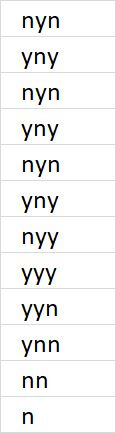
Is there a way to have overlap in counting? I have the string nynynynyyynn and I want to count how many times the pattern nyn exists. When I use the formula provided it counts 2 because it doesn't reuse the n in the 3rd position (or at least that's what I think is happening). Is there a way to get this to be 3?
Meaghan,
Great question!
The substitute function deletes each substring "nyn" from the value, that is why it doesn't "reuse" the n because there is no n.
I made a new formula for you that I believe matches each instance even if overlapping, see this article:
https://www.get-digital-help.com/count-a-given-pattern-in-a-cell-value/
Hi Oscar,
Clear explination! Thanks
If you replace the value in A1 to "AAA" then the answer should be 5
But the formula gives 4, because you substitute the found substring with nothing.
I read your suggestion on https://www.get-digital-help.com/count-a-given-pattern-in-a-cell-value/
That is the right answer for 1 cell.
How do I use this formula for the search of a substring on the "tbl" from your example? Wich should give the answer 5........
Marcel Maatman
It is not possible to build an array with different number of rows and columns, like this:
1 1 1
2 3
1
This is needed for the formula to work. I need to think about this, not sure I can solve it. It can be done with a user defined function.
I want to use the above formula on filtered rows. How can I do that? Any help is appreciated. Thanks!
Dear Oscar,
This is a very helpful formula. My requirement is to use the exact formula but on filtered rows so the rows can change based on the filter condition. Is there an easy fix for this? Any pointers will be helpful. Thanks.
Paras Desai,
great question.
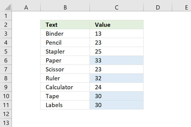
Array formula in cell C3:
=SUM((LEN(IF(SUBTOTAL(103, OFFSET(Table1[Country], MATCH(ROW(Table1[Country]), ROW(Table1[Country]))-1, 0, 1)), Table1[Text]))-LEN(SUBSTITUTE(IF(SUBTOTAL(103, OFFSET(Table1[Country], MATCH(ROW(Table1[Country]), ROW(Table1[Country]))-1, 0, 1)), Table1[Text]), $C$2, "")))/LEN($C$2))
Get the workbook
Count-string-in-a-filtered-table.xlsx
Paras Desai,
You also have the option to let the Excel defined Table do the math.
Formula in cell D5:
=(LEN([@Text])-LEN(SUBSTITUTE([@Text], $C$2, "")))/LEN($C$2)
1. Select any cell in the Excel defined Table.
2. Go to tab Table design.
3. Press with left mouse button on check box "Total row" to show the total.
how to write
in cel a1 to to cell b2
5489 to 4589 what formula to use to arange number in smallest to largest
https://postimg.cc/Mcc7zvt4/7c681b03
I need to count the values in C row which meets criteria in A row.
For example, I want to count only C2:C6 which is 6.9 in row A. count values of C7:C12 which meets criteria as 7 in row A
Can a date range be added to this formula? I need to find it between two dates.