Count cells based on color

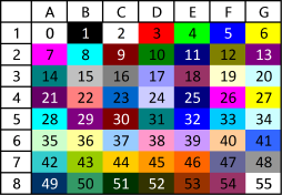
This article explains how to count cells highlighted with Conditional Formatting (CF). The image above shows data in cell range B2:C11, column C has Conditional Formatting applied based on the following CF formula.

A Conditional Formatting formula allows you to create your own condition or criteria if the built-in conditions are not enough.

As far as I know, you can only count cells with cell background color, not font color or bold/italic etc. It is also not possible to count cells highlighted with Conditional Formatting using VBA code, however, you can count cells manually formatted using VBA code.

If you know how to apply Conditional Formatting based on a formula you can skip these steps and go to the next section right now. Here are the steps to apply Conditional Formatting to a cell range.

1. How to apply Conditional Formatting

These steps explain how to apply Conditional Formatting to a cell range based on a formula.

1. Select the cell range you want to highlight.
2. Go to tab "Home" on the ribbon.
3. Press with left mouse button on "Conditional Formatting" button on the ribbon.
4. Press with left mouse button on "New Rule...", a dialog box appears. See the image above.
5. Type your formula in "Format values where this formula is true:".
6. Press with left mouse button on "Format..." button and another dialog box appears.
7. Press with left mouse button on tab "Fill" on the top menu.
8. Pick a color.
9. Press with left mouse button on "OK" button.
10. Press with left mouse button on "OK" button again.

Back to top

2. How to count cells with a specific cell background color [Excel 365]

These steps show how to count highlighted cells.

1. Select any cell in the data set.
2. Press CTRL + T to open "Create Table" dialog box.
   
3. Press with left mouse button on the checkbox accordingly based on the layout of your data set.
4. Press with left mouse button on "OK" button to create the Excel Table.
5. Press with left mouse button on the arrow next to the column name you want count cells in.
   
6. A pop-up menu appears, press with left mouse button on "Filter by Color". Another pop-up menu appears, press with left mouse button on the color you want to sort by.
   
7. The Excel Table now shows only the cells with the selected background color.
8. Select any cell in the Excel Table and a new tab on the ribbon shows up named "Table Design", press with left mouse button on that tab to select it.
9. Press with left mouse button on the checkbox "Total Row" located on the ribbon, see image above. A new row appears below the Excel Table values.
   
10. Press with left mouse button on the number next to total. An arrow appears next to the number, press with left mouse button on that arrow. See image above.
11. Press with left mouse button on "Count".

The number of cells highlighted with a given cell background color using conditional formatting is shown in cell C12.

Back to top

3. How to count cells with a specific cell color [Previous Excel versions]

1. Press with right mouse button on on a cell that has a background color you want to count. A pop-up menu appears.
2. Press with left mouse button on "Sort" and another pop-up menu shows up.
3. Press with mouse on "Put Selected Cell Color On Top".
   
4. Select all colored cells.
   
5. Excel returns the count of your selection in the lower right corner of your Excel window. See image above.

Back to top

4. Count cells with a specific cell background color using the FILTER tool and the SUBTOTAL function [Excel 365]

This section demonstrates how to count cell background color based on Conditional Formatting using the Filter tool. The Filter tool is built-in to Excel, the following steps show you how.

1. Select any cell in your data set.
2. Press shortcut keys CTRL + SHIFT + L to apply the Filter feature to your data set. You know it is there when you have arrows next to your column names. You can also go to tab "Data" on the ribbon and press with left mouse button on "Filter" button to apply it.
3. Press with left mouse button on the arrow in the column you want to count a specific cell background color. A pop-up menu appears.
   
4. Press with mouse on "Filter by Color" and another pop-up menu appears.
5. Press with mouse on the color you want to filter by, see image above.

The following formula will count visible cells in cell range C3:C11 that is not empty. I entered it in cell C13.

The SUBTOTAL function allows you to perform many different calculations based on the first argument. It is also able to perform these calculations to filtered values in contrast to the regular SUM, AVERAGE, COUNT and COUNTA functions.

SUBTOTAL(function_num, ref1, ...)

Back to top

Get the Excel file

Count-cells-with-Conditional-formatting.xlsx

Back to top

Recommended reading

• Conditional Formatting (Excel easy)
• Use conditional formatting to highlight information (Microsoft Ofiice)
• Using If/Then in Conditional Formatting in Excel

6. Count cells based on background color programmatically

This article demonstrates a VBA macro that counts cells based on their background color.

I got a question about counting background colors in a cell range. Excel uses two different properties to color cells and they are ColorIndex and Color property.

The ColorIndex property has 56 different colors, shown below.

The color property holds up to 16 777 216 colors. I tried to color 16 columns with 1048576 rows each (16 * 1048576 = 16 777 216) using the color property but excel returned this error after 65277 cells.

Back to top

6.1. VBA code

The following macro lets you count background colors, however, note that it won't count cells colored with conditional formatting.

'Name macro
Sub CountColors()
'This macro counts background colors in cell range
'https://www.get-digital-help.com/2017/03/30/count-colored-cells/

'Dimension variables and declare data types
Dim IntColors() As Long, i As Integer
Dim chk As Boolean

'Ask user for a cell range and save the output to range variable rng
Set rng = Application.InputBox("Select a cell range to count colors: ", , , , , , , 8)

'Redimension array variable IntColors
ReDim IntColors(0 To 2, 0)

'For Each ... Next statement
For Each cell In rng
chk = False
For c = LBound(IntColors, 2) To UBound(IntColors, 2)
If cell.Interior.ColorIndex = IntColors(0, c) And cell.Interior.Color = IntColors(1, c) Then
IntColors(2, c) = IntColors(2, c) + 1
chk = True
Exit For
End If
Next c

If chk = False Then
IntColors(0, UBound(IntColors, 2)) = cell.Interior.ColorIndex
IntColors(1, UBound(IntColors, 2)) = cell.Interior.Color
ReDim Preserve IntColors(2, UBound(IntColors, 2) + 1)
End If

Next cell

ReDim Preserve IntColors(2, UBound(IntColors, 2) - 1)

Set WS = Sheets.Add

WS.Range("A1") = "Color and count"
WS.Range("B1") = "ColorIndex"
WS.Range("C1") = "Color"
j = 1
For i = LBound(IntColors, 2) To UBound(IntColors, 2)
If IntColors(2, i) <> 0 Then
WS.Range("A1").Offset(j).Interior.ColorIndex = IntColors(0, i)
WS.Range("A1").Offset(j).Interior.Color = IntColors(1, i)
WS.Range("A1").Offset(j) = IntColors(2, i)
WS.Range("A1").Offset(j, 1) = IntColors(0, i)
WS.Range("A1").Offset(j, 2) = IntColors(1, i)
j = j + 1
End If
Next i
End Sub

Back to top

6.2. Where do I copy and paste the VBA code?

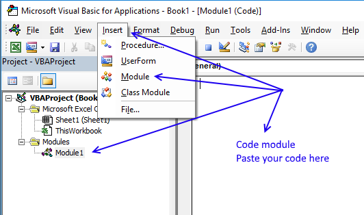
1. Select and copy code above (Ctrl+c).
2. Open VB Editor (Alt+F11).
3. Insert a new module to your workbook.
4. Paste code to code module.

Note, save your workbook with file extension *.xlsm (macro-enabled workbook) to keep the code attached to your workbook.

Back to top

6.3. Instructions

1. Press Alt + F8 to open the macro dialog box, it shows a list of macros currently in your open workbooks.
2. Press with mouse on macro CountColors with left mouse button to slect it.
3. Press the "Run" button on the dialog box.
4. Select a cell range you want to count.

The macro then creates a new sheet with cells in a column colored and their count, see picture below.

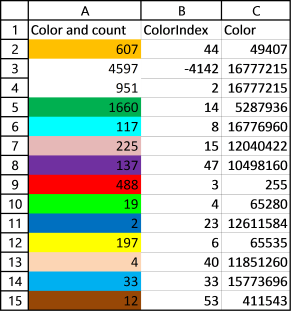
Value -4142  means No fill and -4105 is the default color (white).

There is no way to quickly transfer cell formatting properties to an array so the macro is quite slow, it reads a cell's property one by one. I don't recommend using this with larger cell ranges unless you are prepared to wait for a while.

Back to top

Get the Excel file

Rotating-unique-groups-with-no-repeatv2.xlsx

Back to top

7. Count unique distinct values by cell color - not CF

This article demonstrates a User Defined Function (UDF) that counts unique distinct cell values based on a given cell color. A UDF is an Excel Function that you can build yourself which is very handy if there isn't a built-in function that can do it for you.

A UDF is built of VBA code, VBA stands for Visual Basic for Applications. Microsoft Excel has a built-in Editor named Visual Basic Editor that allows you to create macros and UDFs. You will be surprised how easy it is to start building your own macros.

The image above shows the following formula in cell E4:

The first argument is the cell range. The second argument is a single cell with a color you want to use as a condition. Cell D4 has an interior color red.

The formula in cell E4 uses the color of cell D4 to find cells in cell range B3:B22 with the same color. When a matching color is found the cell value is analyzed and possibly counted in order to count all unique distinct values.

For example, the formula returns 6 in cell E4 because there are 6 numbers in red cells and they all are unique. Cell E6 returns 4, numbers in green cells are 87, 84, 78, 75, 78 and  84. Number 84 and 78 have duplicates. Unique distinct values are all values except duplicates are merged into one single value. That leaves us four numbers: 87, 84, 75 and 78.

The formula above won't work until you have copied the VBA code below and pasted it to a code module in your workbook.

User Defined Syntax

CountC(rng As Range, Cell As Range)

Arguments

VBA code

VBA code is easy to learn, I highly recommend the macro recorder if you are new to VBA. It lets you record a macro based on your actions. Start the recording, perform your actions and then stop the recording. Now, look at the code Excel created.

You can find the "Macro recorder" on the "Developer" tab, if that tab is missing on the ribbon you need to enable it. Then go to the VB Editor to check out the code Excel created for you. See instructions below on how to show the Visual Basic Editor.

I have commented each line in the UDF displayed below, you can copy those lines as well. The apostrophe is a character that allows you to comment your code, it will be ignored when the UDF or macro is started.

'Name the User Defined Function and it's parameters 
Function CountC(rng As Range, Cell As Range)

'Dimension variables and declare data types
Dim CellC As Range, ucoll As New Collection

'Iterate through each cell in range object rng using variable CellC
For Each CellC In rng

    'Check if cell color is equal to second parameter
    If CellC.Interior.Color = Cell.Interior.Color Then

        'Enable error handling
        On Error Resume Next

            'Check if the number of characters are larger than zero and if so add the cell value to collection ucoll
            If Len(CellC) > 0 Then ucoll.Add CellC, CStr(CellC)

        'Disable error handling
        On Error GoTo 0
    End If

'Continue with next cell
Next CellC

'Return values in collection variable ucoll to UDF
CountC = ucoll.Count
End Function

I do recommend commenting your VBA code, it will be a time saver next time you need the macro/UDF and need to do modifications.

Where to put the code?

The image above shows the Visual Basic Editor. The Project Explorer is to the left and an empty window is to the right. There is a top menu and some buttons below the top menu.

The image shows what to press with left mouse button on in order to create a new module in your workbook for the User Defined Function.

1. Copy above VBA code.
2. Press shortcut keys Alt + F11 to open the Visual Basic Editor. The Project Explorer window is to the left, it allows you to select which workbook and module to use.
3. Press with left mouse button on "Insert" on the top menu.
4. Press with left mouse button on "Module" to create a code module in your workbook.
5. Paste to code window, see image above.
6. Exit VB Editor and return to Excel.

Get the Excel file

Count-unique-distinct-values-in-colored-cells.xlsm

Recommended articles

• How to Count Colored Cells in Excel
• How to count and sum cells by color in Excel

8. How to change cell background color

Excel lets you color cells using the "Fill Color" tool located on tab "Home" on the ribbon.

1. Select the cell or cell range you want to apply a different background color to.
2. Go to tab "Home" on the ribbon.
3. Press with left mouse button on "Fill Color" button and a pop-up menu appears.
4. Pick a color.

Sometimes it can be useful to know the number of cells filled with a specific background color. Excel 365 makes this really easy, there is a work-around for older Excel versions that I will show in this article as well.

Back to top

9. How to count cells with a specific background-color (Excel 365)

The Excel Table allows you to filter and count cells with a specific background color.

1. Select any cell in the data set.
2. Press shortcut keys CTRL + T to show the "Create Table" dialog box.
   
3. Enable the checkbox if your data has header names.
4. Press with left mouse button on the "OK" button to convert cell range to an Excel Table.

1. Press with left mouse button on the arrow next to the header name which corresponds to the column you want to filter.
2. A pop-up menu appears, press with left mouse button on "Filter by Color".
3. Another pop-up menu appears, press with left mouse button on the color you want to filter by.

1. Select any cell in the Excel Table. A new tab shows up on the ribbon named "Table Design".
2. Press with mouse on the tab "Table Design" on the ribbon.
3. Press with mouse on checkbox "Total Row", see image above.

A new cell appears below the Excel Table, see image above.

1. Select the new cell. An arrow appears next to the number, see image above.
2. Press with left mouse button on the "Arrow", a pop-up menu appears.
3. Press with left mouse button on "Count".

The number in the cell changes, it now shows the total count of cells based on the filter we applied. The formula bars hows this formula:

The SUBTOTAL function is able to count visible cells in a filtered table, number 103 stands for COUNT and [Numbers] is a structured reference to data in column Numbers.

Structured references appear automatically when you reference data in an Excel Table, in this case, Excel created this for us when we enabled checkbox "Total row" in a previous step.

Back to top

10. How to count cells with a specific background-color (earlier Excel versions)

1. Press with right mouse button on on a cell that has the background color you want to filter by. A pop-up menu appears.
   
2. Press with mouse on "Sort", another pop-up menu shows up.
3. Press with left mouse button on "Put selected Cell color on top".

The data is now sorted by cell color, see image above. Select all cells with the background color you want to count, they should now be adjacent to each other and sorted on top.

Excel counts the selected cells for and shows the number in the lower right corner of your Excel window.

Back to top

11. Count cells by cell font properties (font color, cell color, bold or italic)

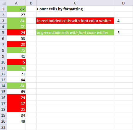
The image above demonstrates a User defined function (UDF) in cell D3 that counts cells in column A based on the cell formatting in cell C3. The font properties are color, cell color and bold/italic.

Custom function in cell D3:

The user defined function counts how many times the font properties in cell C3 match each cell in the cell range A1:A20.

User defined function

'Name UDF and dimension parameters and declare their data types
Function CountC(rng As Range, Cell As Range)

'Dimension variables and declare data types
Dim CellC As Range, ucoll As New Collection, i As Single

'Save 0 (zero) to variable i
i = 0

'Iterate through each cell in parameter rng using variable CellC
For Each CellC In rng
    'Check if cell background color matches parameter Cell's cell background color
    If CellC.Interior.Color = Cell.Interior.Color And _
    CellC.Font.Bold = Cell.Font.Bold And _
    CellC.Font.Italic = Cell.Font.Italic And _
    CellC.Font.ColorIndex = Cell.Font.ColorIndex Then
        'Add 1 to the number in variable i
        i = i + 1
    End If

'Continue with next cell
Next CellC

'Return number stored in variable i to UDF.
CountC = i

End Function

Back to top

Where to put the VBA code?

1. Copy VBA code.
2. Press Alt + F11 to open the VB Editor.
3. Press with left mouse button on "Insert" on the top menu, a pop-up menu appears. See image above.
4. Press with left mouse button on "Module" to insert a module to your workbook. The module appears in the "Project Explorer", in this case, named Module1.
5. Paste code to code window.

Back to top

12. Count unique distinct cells by cell font properties (font color, cell color, bold or italic)

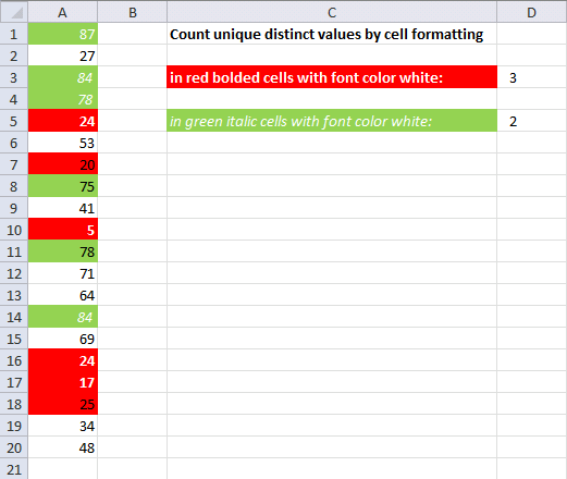
The image above shows a user defined function in cell D3 that counts unique distinct values in cell range A1:A20 based on the cell formatting in cell C3. This UDF also checks font color, cell color and bold/italic.

The formula in cell D3 returns 3 because the values in cell A5, A10, A16 and A17 match the cell formatting in cell C3. The values are 24, 5, 24 and 17. However, the unique distinct values are 24, 5 and 17. 3 numbers and 3 is returned to cell D3.

Custom function in cell D3:

The user defined function matches the font properties in cell C3 with each cell in cell range A1:A20, then counts unique distinct values in those matching cells.

User defined function

Function CountUDC(rng As Range, Cell As Range)
Dim CellC As Range, ucoll As New Collection
For Each CellC In rng
    If CellC.Interior.Color = Cell.Interior.Color And _
    CellC.Font.Bold = Cell.Font.Bold And _
    CellC.Font.Italic = Cell.Font.Italic And _
    CellC.Font.ColorIndex = Cell.Font.ColorIndex Then
        On Error Resume Next
            If Len(CellC) > 0 Then ucoll.Add CellC, CStr(CellC)
        On Error GoTo 0
    End If
Next CellC
CountUDC = ucoll.Count
End Function

Back to top

Get Excel file

Get the Excel file

Count-values-and-unique-distinct-values-by-cell-formating.xlsm

Back to top

Recommended reading

Built-in conditional formatting

Highlight cells rule

Top bottom rules

Basic CF formulas

Search using CF

Unique distinct

Duplicates

Compare

Min max

Dates

Misc

Excel categories

Comments (47)