Extract duplicates from a multi-column cell range
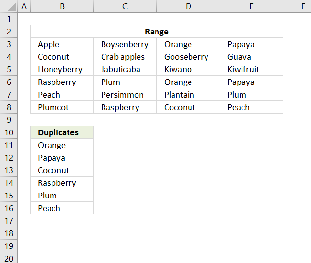
This article describes two formulas that extract duplicates from a multi-column cell range, the first one is built for Excel 365 and the second one is for earlier versions.
If your values are in a column only then there are much smaller and easier formulas to use: Extract a list of duplicates from a column
Table of Contents
1. Extract duplicates from a range - Excel 365
Excel 365 formula in cell B11:
Explaining formula in cell B11
Step 1 - Count values
The COUNTIF function calculates the number of cells that is equal to a condition.
Function syntax: COUNTIF(range, criteria)
COUNTIF(B3:E8, B3:E8)
becomes
COUNTIF({"Apple", "Boysenberry", "Orange", "Papaya";"Coconut", "Crab apples", "Gooseberry", "Guava";"Honeyberry", "Jabuticaba", "Kiwano", "Kiwifruit";"Raspberry", "Plum", "Orange", "Papaya";"Peach", "Persimmon", "Plantain", "Plum";"Plumcot", "Raspberry", "Coconut", "Peach"}, {"Apple", "Boysenberry", "Orange", "Papaya";"Coconut", "Crab apples", "Gooseberry", "Guava";"Honeyberry", "Jabuticaba", "Kiwano", "Kiwifruit";"Raspberry", "Plum", "Orange", "Papaya";"Peach", "Persimmon", "Plantain", "Plum";"Plumcot", "Raspberry", "Coconut", "Peach"}))
and returns
{1,1,2,2;2,1,1,1;1,1,1,1;2,2,2,2;2,1,1,2;1,2,2,2}
A number above 1 tells us the value is a duplicate.
Step 2 - Rearrange numbers
The TOCOL function rearranges values in 2D cell ranges to a single column.
Function syntax: TOCOL(array, [ignore], [scan_by_col])
TOCOL(COUNTIF(B3:E8, B3:E8))
becomes
TOCOL({1,1,2,2;2,1,1,1;1,1,1,1;2,2,2,2;2,1,1,2;1,2,2,2})
and returns
{1;1;2;2;2;1;1;1;1;1;1;1;2;2;2;2;2;1;1;2;1;2;2;2}
Step 3 - Check if number is larger than 1
The larger sign is a logical operator that returns TRUE if condition is met and FALSE if not.
TOCOL(COUNTIF(B3:E8, B3:E8))>1
becomes
{1;1;2;2;2;1;1;1;1;1;1;1;2;2;2;2;2;1;1;2;1;2;2;2}>1
and returns
{FALSE; FALSE; TRUE; TRUE; TRUE; FALSE; FALSE; FALSE; FALSE; FALSE; FALSE; FALSE; TRUE; TRUE; TRUE; TRUE; TRUE; FALSE; FALSE; TRUE; FALSE; TRUE; TRUE; TRUE}
Step 4 - Rearrange text values
TOCOL(B3:E8)
becomes
TOCOL({"Apple", "Boysenberry", "Orange", "Papaya";"Coconut", "Crab apples", "Gooseberry", "Guava";"Honeyberry", "Jabuticaba", "Kiwano", "Kiwifruit";"Raspberry", "Plum", "Orange", "Papaya";"Peach", "Persimmon", "Plantain", "Plum";"Plumcot", "Raspberry", "Coconut", "Peach"})
and returns
{"Apple"; "Boysenberry"; "Orange"; "Papaya"; "Coconut"; "Crab apples"; "Gooseberry"; "Guava"; "Honeyberry"; "Jabuticaba"; "Kiwano"; "Kiwifruit"; "Raspberry"; "Plum"; "Orange"; "Papaya"; "Peach"; "Persimmon"; "Plantain"; "Plum"; "Plumcot"; "Raspberry"; "Coconut"; "Peach"}
Step 5 - Filter duplicate values
The FILTER function extracts values/rows based on a condition or criteria.
Function syntax: FILTER(array, include, [if_empty])
FILTER(TOCOL(B3:E8), TOCOL(COUNTIF(B3:E8, B3:E8))>1)
becomes
FILTER({"Apple"; "Boysenberry"; "Orange"; "Papaya"; "Coconut"; "Crab apples"; "Gooseberry"; "Guava"; "Honeyberry"; "Jabuticaba"; "Kiwano"; "Kiwifruit"; "Raspberry"; "Plum"; "Orange"; "Papaya"; "Peach"; "Persimmon"; "Plantain"; "Plum"; "Plumcot"; "Raspberry"; "Coconut"; "Peach"}, {FALSE; FALSE; TRUE; TRUE; TRUE; FALSE; FALSE; FALSE; FALSE; FALSE; FALSE; FALSE; TRUE; TRUE; TRUE; TRUE; TRUE; FALSE; FALSE; TRUE; FALSE; TRUE; TRUE; TRUE})
and returns
{"Orange"; "Papaya"; "Coconut"; "Raspberry"; "Plum"; "Orange"; "Papaya"; "Peach"; "Plum"; "Raspberry"; "Coconut"; "Peach"}
Step 6 - Show only one instance of each duplicate
The UNIQUE function returns a unique or unique distinct list.
Function syntax: UNIQUE(array,[by_col],[exactly_once])
UNIQUE(FILTER(TOCOL(B3:E8), TOCOL(COUNTIF(B3:E8, B3:E8))>1))
becomes
UNIQUE({"Orange"; "Papaya"; "Coconut"; "Raspberry"; "Plum"; "Orange"; "Papaya"; "Peach"; "Plum"; "Raspberry"; "Coconut"; "Peach"})
and returns
{"Orange";"Papaya";"Coconut";"Raspberry";"Plum";"Peach"}.
2. Extract duplicates from a range
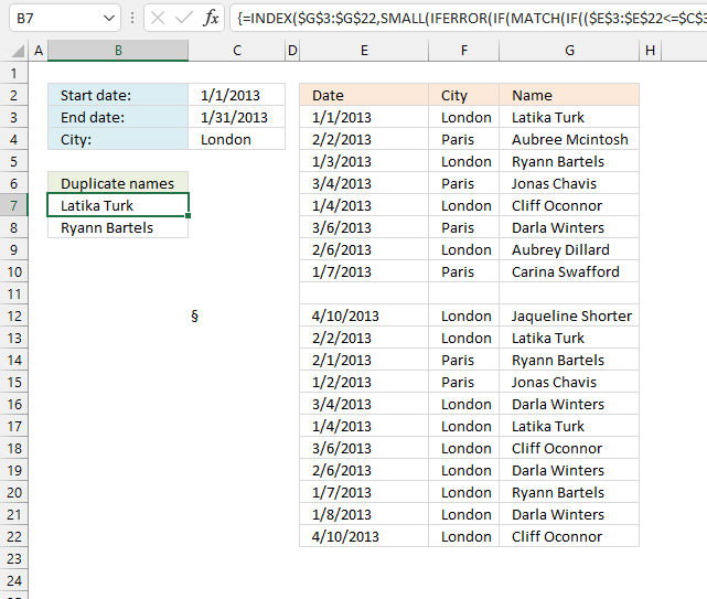
The following array formula in cell B11 extracts duplicates from cell range B3:E8, only one instance of each duplicate is returned.
Array formula in cell B11:
To enter an array formula, type the formula in a cell then press and hold CTRL + SHIFT simultaneously, now press Enter once. Release all keys.
The formula bar now shows the formula with a beginning and ending curly bracket telling you that you entered the formula successfully. Don't enter the curly brackets yourself.
Explaining formula in cell B11
This formula consists of two parts, one extracts the row number and the other the column number needed to return the correct value.
INDEX(reference, row, col)
Step 1 to 6 shows how the row number is calculated, step 7 to 11 demonstrates how to calculate the column number.
Step 1 - Show one instance of each duplicate
The COUNTIF function counts values based on a condition or criteria, in this case, we take into account previously displayed values in order to prevent duplicates in our output list.
COUNTIF($B$10:B10, $B$3:$E$8)
becomes
COUNTIF("Duplicates", {"Apple", "Boysenberry", "Orange", "Papaya";"Coconut", "Crab apples", "Gooseberry", "Guava";"Honeyberry", "Jabuticaba", "Kiwano", "Kiwifruit";"Raspberry", "Plum", "Orange", "Papaya";"Peach", "Persimmon", "Plantain", "Plum";"Plumcot", "Raspberry", "Coconut", "Peach"})
and returns
{0,0,0,0; 0,0,0,0; 0,0,0,0; 0,0,0,0; 0,0,0,0; 0,0,0,0}
Step 2 - Find duplicates
(COUNTIF($B$3:$E$8, $B$3:$E$8)<2)
becomes
({1,1,2,2;2,1,1,1;1,1,1,1;2,2,2,2;2,1,1,2;1,2,2,2}<2)
and returns
{TRUE,TRUE, FALSE,FALSE; FALSE,TRUE, TRUE,TRUE; TRUE,TRUE, TRUE,TRUE; FALSE,FALSE, FALSE,FALSE; FALSE,TRUE, TRUE,FALSE; TRUE,FALSE, FALSE,FALSE}
Step 3 - Add arrays
The parentheses makes sure that the arrays are added before comparing to 0 (zero).
(COUNTIF($B$10:B10, $B$3:$E$8)+(COUNTIF($B$3:$E$8, $B$3:$E$8)<2))=0
becomes
({0,0,0,0; 0,0,0,0; 0,0,0,0; 0,0,0,0; 0,0,0,0; 0,0,0,0}+{TRUE,TRUE, FALSE,FALSE; FALSE,TRUE, TRUE,TRUE; TRUE,TRUE, TRUE,TRUE; FALSE,FALSE, FALSE,FALSE; FALSE,TRUE, TRUE,FALSE; TRUE,FALSE, FALSE,FALSE})=0
becomes
{1,1,0,0;0,1,1,1;1,1,1,1;0,0,0,0;0,1,1,0;1,0,0,0}=0
and returns
{FALSE, FALSE, TRUE, TRUE;TRUE, FALSE, FALSE, FALSE;FALSE, FALSE, FALSE, FALSE;TRUE, TRUE, TRUE, TRUE;TRUE, FALSE, FALSE, TRUE;FALSE, TRUE, TRUE, TRUE}.
Step 4 - Replace TRUE with the corresponding row number
The IF function uses a logical expression to determine which value (argument) to return.
IF((COUNTIF($B$10:B10, $B$3:$E$8)+(COUNTIF($B$3:$E$8, $B$3:$E$8)<2))=0, ROW($B$3:$E$8)-MIN(ROW($B$3:$E$8))+1)
becomes
IF({FALSE, FALSE, TRUE, TRUE;TRUE, FALSE, FALSE, FALSE;FALSE, FALSE, FALSE, FALSE;TRUE, TRUE, TRUE, TRUE;TRUE, FALSE, FALSE, TRUE;FALSE, TRUE, TRUE, TRUE}, ROW($B$3:$E$8)-MIN(ROW($B$3:$E$8))+1)
becomes
IF({FALSE, FALSE, TRUE, TRUE;TRUE, FALSE, FALSE, FALSE;FALSE, FALSE, FALSE, FALSE;TRUE, TRUE, TRUE, TRUE;TRUE, FALSE, FALSE, TRUE;FALSE, TRUE, TRUE, TRUE}, {1;2;3;4;5;6})
and returns
{FALSE,FALSE, 1,1; 2,FALSE,FALSE,FALSE; FALSE,FALSE,FALSE,FALSE; 4,4,4,4; 5,FALSE,FALSE,5; FALSE,6,6,6}
Step 5 - Find smallest value
The MIN function finds the minimum value in the array ignoring the boolean values.
MIN(IF((COUNTIF($B$10:B10, $B$3:$E$8)+(COUNTIF($B$3:$E$8, $B$3:$E$8)<2))=0, ROW($B$3:$E$8)-MIN(ROW($B$3:$E$8))+1))
becomes
MIN({FALSE,FALSE, 1,1; 2,FALSE,FALSE,FALSE; FALSE,FALSE,FALSE,FALSE; 4,4,4,4; 5,FALSE,FALSE,5; FALSE,6,6,6})
and returns 1. This tells us that the first duplicate value is somewhere on row 1 in cell range B3:E8.
Step 6 - Return the row number of the first duplicate
This step is the same as step 1 to 5 and is repeated in order to get all values from the row.
MIN(IF((COUNTIF($B$10:B10, $B$3:$E$8)+IF(COUNTIF($B$3:$E$8, $B$3:$E$8)>1, 0, 1))=0, ROW($B$3:$E$8)-MIN(ROW($B$3:$E$8))+1))
returns 1.
Step 7 - Extract values from row
INDEX($B$3:$E$8, MIN(IF((COUNTIF($B$10:B10, $B$3:$E$8)+IF(COUNTIF($B$3:$E$8, $B$3:$E$8)>1, 0, 1))=0, ROW($B$3:$E$8)-MIN(ROW($B$3:$E$8))+1)), , 1)
becomes
INDEX($B$3:$E$8, 1, , 1)
and returns
{"Apple","Boysenberry","Orange","Papaya"}.
Step 8 - Check if the values have been displayed in cells above
(COUNTIF($B$10:B10, INDEX($B$3:$E$8, MIN(IF((COUNTIF($B$10:B10, $B$3:$E$8)+IF(COUNTIF($B$3:$E$8, $B$3:$E$8)>1, 0, 1))=0, ROW($B$3:$E$8)-MIN(ROW($B$3:$E$8))+1)), , 1))<>0)
becomes
(COUNTIF($B$10:B10, {"Apple","Boysenberry","Orange","Papaya"})<>0)
becomes
({0,0,0,0}<>0)
and returns
{FALSE,FALSE,FALSE,FALSE}.
Step 9 - Identify duplicates on the same row
(COUNTIF($B$3:$E$8, INDEX($B$3:$E$8, MIN(IF((COUNTIF($B$10:B10, $B$3:$E$8)+IF(COUNTIF($B$3:$E$8, $B$3:$E$8)>1, 0, 1))=0, ROW($B$3:$E$8)-MIN(ROW($B$3:$E$8))+1)), , 1))<2)
becomes
(COUNTIF($B$3:$E$8, {"Apple","Boysenberry","Orange","Papaya"})<2)
becomes
({1,1,2,2}<2)
and returns
{TRUE,TRUE,FALSE,FALSE}.
This tells us that there are two duplicates on row 1.
Step 10 - Add arrays
(COUNTIF($B$10:B10, INDEX($B$3:$E$8, MIN(IF((COUNTIF($B$10:B10, $B$3:$E$8)+IF(COUNTIF($B$3:$E$8, $B$3:$E$8)>1, 0, 1))=0, ROW($B$3:$E$8)-MIN(ROW($B$3:$E$8))+1)), , 1))<>0)+(COUNTIF($B$3:$E$8, INDEX($B$3:$E$8, MIN(IF((COUNTIF($B$10:B10, $B$3:$E$8)+IF(COUNTIF($B$3:$E$8, $B$3:$E$8)>1, 0, 1))=0, ROW($B$3:$E$8)-MIN(ROW($B$3:$E$8))+1)), , 1))<2)
becomes
{FALSE,FALSE,FALSE,FALSE} + {TRUE,TRUE,FALSE,FALSE}
and returns
{1,1,0,0}
Step 11 - Identify duplicate and return relative column number
MATCH(0, IF(COUNTIF($B$10:B10, INDEX($B$3:$E$8, MIN(IF((COUNTIF($B$10:B10, $B$3:$E$8)+IF(COUNTIF($B$3:$E$8, $B$3:$E$8)>1, 0, 1))=0, ROW($B$3:$E$8)-MIN(ROW($B$3:$E$8))+1)), , 1))=0, 0, 1)+IF(COUNTIF($B$3:$E$8, INDEX($B$3:$E$8, MIN(IF((COUNTIF($B$10:B10, $B$3:$E$8)+IF(COUNTIF($B$3:$E$8, $B$3:$E$8)>1, 0, 1))=0, ROW($B$3:$E$8)-MIN(ROW($B$3:$E$8))+1)), , 1))>1, 0, 1), 0)
becomes
MATCH(0, {1,1,0,0}, 0)
and returns 3.
Step 12 - Return value
The INDEX function returns a value based on a row and column number.
=INDEX($B$3:$E$8, MIN(IF((COUNTIF($B$10:B10, $B$3:$E$8)+(COUNTIF($B$3:$E$8, $B$3:$E$8)<2))=0, ROW($B$3:$E$8)-MIN(ROW($B$3:$E$8))+1)), MATCH(0, (COUNTIF($B$10:B10, INDEX($B$3:$E$8, MIN(IF((COUNTIF($B$10:B10, $B$3:$E$8)+IF(COUNTIF($B$3:$E$8, $B$3:$E$8)>1, 0, 1))=0, ROW($B$3:$E$8)-MIN(ROW($B$3:$E$8))+1)), , 1))<>0)+(COUNTIF($B$3:$E$8, INDEX($B$3:$E$8, MIN(IF((COUNTIF($B$10:B10, $B$3:$E$8)+IF(COUNTIF($B$3:$E$8, $B$3:$E$8)>1, 0, 1))=0, ROW($B$3:$E$8)-MIN(ROW($B$3:$E$8))+1)), , 1))<2), 0))
becomes
=INDEX($B$3:$E$8, 1, 3)
and returns "Orange" in cell D3.
Get Excel *.xlsx file
Extract duplicates from a multicolumn rangev2.xlsx
3. Filter duplicate values from a range that begins with string
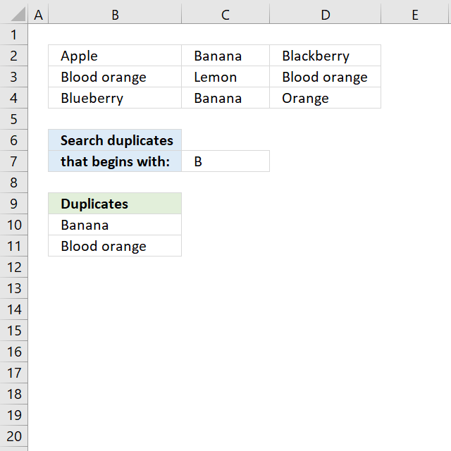
The array formula in cell B10 extracts duplicate values from cell range B2:D4 if they begin with the condition specified in cell C7.
Array formula in B10:
copied down as far as needed.
Excel 365 formula in cell B11:
Explaining formula in cell B10
Step 1 - Identify values beginning with search string
The LEFT function returns a given number of characters from the start of a text string.
LEFT($B$2:$D$4, LEN($C$7))=$C$7
becomes
LEFT({"Apple","Banana","Blackberry";"Blood orange", "Lemon","Blood orange"; "Blueberry","Banana", "Orange"}, LEN($C$7))=$C$7
becomes
LEFT({"Apple","Banana","Blackberry";"Blood orange", "Lemon","Blood orange"; "Blueberry","Banana", "Orange"}, 1)=$C$7
becomes
{"Ap","Ba","Bl"; "Or","Le","Bl"; "Bl","Ba","Or"}=$C$7
becomes
{"A","B","B";"B","L","B";"B","B","O"}="B"
and returns
{FALSE,TRUE, TRUE;TRUE, FALSE,TRUE; TRUE,TRUE, FALSE}.
Step 2 - Keep track of previous values
The COUNTIF function counts values based on a condition or criteria, the first argument contains an expanding cell reference, it grows when the cell is copied to cells below. This makes the formula aware of values displayed in cells above.
COUNTIF(B9:$B$9, $B$2:$D$4)=0
becomes
COUNTIF("Duplicates", {"Apple","Banana","Blackberry";"Blood orange", "Lemon","Blood orange"; "Blueberry","Banana", "Orange"})=0
becomes
{0,0,0;0,0,0;0,0,0}=0
and returns
{TRUE,TRUE,TRUE; TRUE,TRUE,TRUE; TRUE,TRUE,TRUE}.
Step 3 - Identify duplicates
The COUNTIF function counts values based on a condition or criteria, this can be used to find duplicate values.
COUNTIF($B$2:$D$4, $B$2:$D$4)>1
becomes
COUNTIF({"Apple","Banana","Blackberry";"Blood orange", "Lemon","Blood orange"; "Blueberry","Banana", "Orange"}, {"Apple","Banana", "Blackberry";"Blood orange", "Lemon","Blood orange"; "Blueberry","Banana", "Orange"})>1
becomes
{1,2,1;2,1,2;1,2,1}>1
and returns
{FALSE,TRUE, FALSE;TRUE, FALSE,TRUE; FALSE,TRUE, FALSE}.
Step 4 - Multiply arrays
Both values must be true in order to get the value in a later step.
(LEFT($B$2:$D$4, LEN($C$7))=$C$7)*(COUNTIF(B9:$B$9, $B$2:$D$4)=0)*(COUNTIF($B$2:$D$4, $B$2:$D$4)>1)
becomes
{FALSE,TRUE, TRUE;TRUE, FALSE,TRUE; TRUE,TRUE, FALSE}* {TRUE,TRUE,TRUE; TRUE,TRUE,TRUE; TRUE,TRUE,TRUE}* {FALSE,TRUE, FALSE;TRUE, FALSE,TRUE; FALSE,TRUE, FALSE}
and returns
{0,1,0;1,0,1;0,1,0}
Step 5 - Replace TRUE with unique number
The IF function returns a unique number if boolean value is TRUE. FALSE returns "" (nothing). The unique number is needed to find the right value in a later step.
IF((LEFT($B$2:$D$4, LEN($C$7))=$C$7)*(COUNTIF(B9:$B$9, $B$2:$D$4)=0), (ROW($B$2:$D$4)+(1/(COLUMN($B$2:$D$4)+1)))*1, "")
becomes
IF({0,1,0;1,0,1;0,1,0}, (ROW($B$2:$D$4)+(1/(COLUMN($B$2:$D$4)+1)))*1, "")
becomes
IF({0,1,0;1,0,1;0,1,0}, {2.33333333333333, 2.25, 2.2; 3.33333333333333, 3.25, 3.2; 4.33333333333333, 4.25, 4.2}, "")
and returns
{"",2.25,"";3.33333333333333,"",3.2;"",4.25,""}
Step 6 - Find smallest value in array
The MIN function returns the smallest number in array ignoring blanks and text values.
MIN(IF((LEFT($B$2:$D$4, LEN($C$7))=$C$7)*(COUNTIF(B9:$B$9, $B$2:$D$4)=0)*(COUNTIF($B$2:$D$4, $B$2:$D$4)>1), (ROW($B$2:$D$4)+(1/(COLUMN($B$2:$D$4)+1)))*1, ""))
becomes
MIN({"",2.25,"";3.33333333333333,"",3.2;"",4.25,""})
and returns 2.25.
Step 7 - Find corresponding value
IF(MIN(IF((LEFT($B$2:$D$4, LEN($C$7))=$C$7)*(COUNTIF(B9:$B$9, $B$2:$D$4)=0)*(COUNTIF($B$2:$D$4, $B$2:$D$4)>1), (ROW($B$2:$D$4)+(1/(COLUMN($B$2:$D$4)+1)))*1, ""))=(ROW($B$2:$D$4)+(1/(COLUMN($B$2:$D$4)+1)))*1, $B$2:$D$4, "")
becomes
IF(2.25={"",2.25,"";3.33333333333333,"",3.2;"",4.25,""}, $B$2:$D$4, "")
becomes
IF({FALSE,TRUE, FALSE;FALSE, FALSE,FALSE; FALSE,FALSE, FALSE}, $B$2:$D$4, "")
and returns
{"","Banana","";"","","";"","",""}
Step 8 - Concatenate strings in array
The TEXTJOIN function returns values concatenated ignoring blanks in array.
TEXTJOIN("", TRUE, IF(MIN(IF((LEFT($B$2:$D$4, LEN($C$7))=$C$7)*(COUNTIF(B9:$B$9, $B$2:$D$4)=0)*(COUNTIF($B$2:$D$4, $B$2:$D$4)>1), (ROW($B$2:$D$4)+(1/(COLUMN($B$2:$D$4)+1)))*1, ""))=(ROW($B$2:$D$4)+(1/(COLUMN($B$2:$D$4)+1)))*1, $B$2:$D$4, ""))
becomes
TEXTJOIN("", TRUE, {"","Banana","";"","","";"","",""})
and returns "Banana" in cell B10.
Get Excel *.xlsx file
Filter duplicate text values in a range using begins with criterion.xlsx
4. Filter duplicate values in a range that contain a given condition
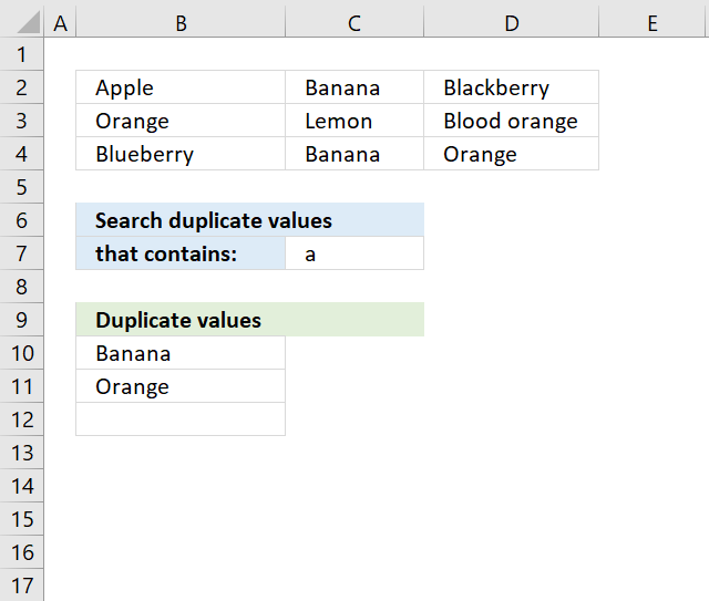
The array formula in cell B10 extracts duplicate values from cell range B2:D4 if they contain string specified in cell C7.
Excel 365 dynamic array formula in cell B10:
Array formula in B10:
To enter an array formula, type the formula in a cell then press and hold CTRL + SHIFT simultaneously, now press Enter once. Release all keys.
The formula bar now shows the formula with a beginning and ending curly bracket telling you that you entered the formula successfully. Don't enter the curly brackets yourself.
Explaining formula in cell B10
Step 1 - Identify values containing search string
The SEARCH function returns a number representing the location of a text string in another string.
ISNUMBER(SEARCH($C$7,$B$2:$D$4))
becomes
ISNUMBER(SEARCH("a",{"Apple", "Banana", "Blackberry"; "Orange", "Lemon", "Blood orange"; "Blueberry", "Banana", "Orange"}))
becomes
ISNUMBER({1,2,3;3,#VALUE!,9;#VALUE!,2,3})
and returns
{TRUE,TRUE, TRUE;TRUE, FALSE,TRUE; FALSE,TRUE, TRUE}
Step 2 - Keep track of previous values
The COUNTIF function counts values based on a condition or criteria, the first argument contains an expanding cell reference, it grows when the cell is copied to cells below. This makes the formula aware of values displayed in cells above. 0 (zero) indicates values that not yet have been displayed
COUNTIF(B9:$B$9,$B$2:$D$4)=0
becomes
COUNTIF("Unique distinct values", {"Apple", "Banana", "Blackberry";"Orange", "Lemon", "Blood orange";"Blueberry", "Banana", "Orange"})=0
becomes
{0,0,0;0,0,0;0,0,0}=0
and returns
{TRUE,TRUE,TRUE; TRUE,TRUE,TRUE; TRUE,TRUE,TRUE}.
Step 3 - Identify duplicates
The COUNTIF function counts values based on a condition or criteria, a value is larger than 1 indicates a dupilcate.
COUNTIF($B$2:$D$4,$B$2:$D$4)>1
becomes
COUNTIF({"Apple", "Banana", "Blackberry";"Orange", "Lemon", "Blood orange";"Blueberry", "Banana", "Orange"}, {"Apple", "Banana", "Blackberry";"Orange", "Lemon", "Blood orange";"Blueberry", "Banana", "Orange"})>1
becomes
{1,2,1;2,1,1;1,2,2}>1
and returns
{FALSE,TRUE, FALSE;TRUE, FALSE,FALSE; FALSE,TRUE, TRUE}.
Step 4 - Multiply arrays
All three corresponding values must be true in order to get the value in a later step.
(COUNTIF(B9:$B$9, $B$2:$D$4)=0)*ISNUMBER(SEARCH($C$7, $B$2:$D$4))*(COUNTIF($B$2:$D$4, $B$2:$D$4)>1)
becomes
{TRUE,TRUE, TRUE;TRUE, FALSE,TRUE; FALSE,TRUE, TRUE}*{TRUE,TRUE,TRUE; TRUE,TRUE,TRUE; TRUE,TRUE,TRUE}* {FALSE,TRUE, FALSE;TRUE, FALSE,FALSE; FALSE,TRUE, TRUE}
and returns
{0,1,0; 1,0,0; 0,1,1}
Step 5 - Replace TRUE with unique number
The IF function returns a unique number if boolean value is TRUE. FALSE returns "" (nothing). The unique number is needed to find the right value in a later step.
IF((COUNTIF(B9:$B$9, $B$2:$D$4)=0)*ISNUMBER(SEARCH($C$7, $B$2:$D$4))*(COUNTIF($B$2:$D$4, $B$2:$D$4)>1), (ROW($B$2:$D$4)+(1/(COLUMN($B$2:$D$4)+1)))*1, "")
becomes
IF({0,1,0; 1,0,0; 0,1,1}, (ROW($B$2:$D$4)+(1/(COLUMN($B$2:$D$4)+1)))*1, "")
becomes
IF({0,1,0; 1,0,0; 0,1,1}, {2.33333333333333, 2.25, 2.2; 3.33333333333333, 3.25, 3.2; 4.33333333333333, 4.25, 4.2}, "")
and returns
{"",2.25,""; 3.33333333333333,"",""; "",4.25,4.2}
Step 6 - Find smallest value in array
The MIN function returns the smallest number in array ignoring blanks and text values.
MIN(IF((COUNTIF(B9:$B$9, $B$2:$D$4)=0)*ISNUMBER(SEARCH($C$7, $B$2:$D$4))*(COUNTIF($B$2:$D$4, $B$2:$D$4)>1), (ROW($B$2:$D$4)+(1/(COLUMN($B$2:$D$4)+1)))*1, ""))
becomes
MIN({"",2.25,""; 3.33333333333333,"",""; "",4.25,4.2})
and returns 2.25.
Step 7 - Find corresponding value
IF(MIN(IF((COUNTIF(B9:$B$9, $B$2:$D$4)=0)*ISNUMBER(SEARCH($C$7, $B$2:$D$4))*(COUNTIF($B$2:$D$4, $B$2:$D$4)>1), (ROW($B$2:$D$4)+(1/(COLUMN($B$2:$D$4)+1)))*1, ""))=(ROW($B$2:$D$4)+(1/(COLUMN($B$2:$D$4)+1)))*1,$B$2:$D$4,"")
becomes
IF(2.2={2.33333333333333, 2.25, 2.2; 3.33333333333333, 3.25, 3.2; 4.33333333333333, 4.25, 4.2}, $B$2:$D$4, "")
becomes
IF({FALSE,FALSE,TRUE; FALSE,FALSE,FALSE; FALSE,FALSE,FALSE}, $B$2:$D$4, "")
and returns
{"","","Banana";"","","";"","",""}
Step 8 - Concatenate strings in array
The TEXTJOIN function returns values concatenated ignoring blanks in array.
TEXTJOIN("",TRUE,IF(MIN(IF((COUNTIF(B9:$B$9,$B$2:$D$4)=0)*ISNUMBER(SEARCH($C$7,$B$2:$D$4)),(ROW($B$2:$D$4)+(1/(COLUMN($B$2:$D$4)+1)))*1,""))=(ROW($B$2:$D$4)+(1/(COLUMN($B$2:$D$4)+1)))*1,$B$2:$D$4,""))
becomes
TEXTJOIN("", TRUE, {"","","Banana";"","","";"","",""})
and returns "Banana" in cell B10.
Get Excel *.xlsx file
Filter duplicate values in a range using a contain conditionv2.xlsx
Duplicate values category
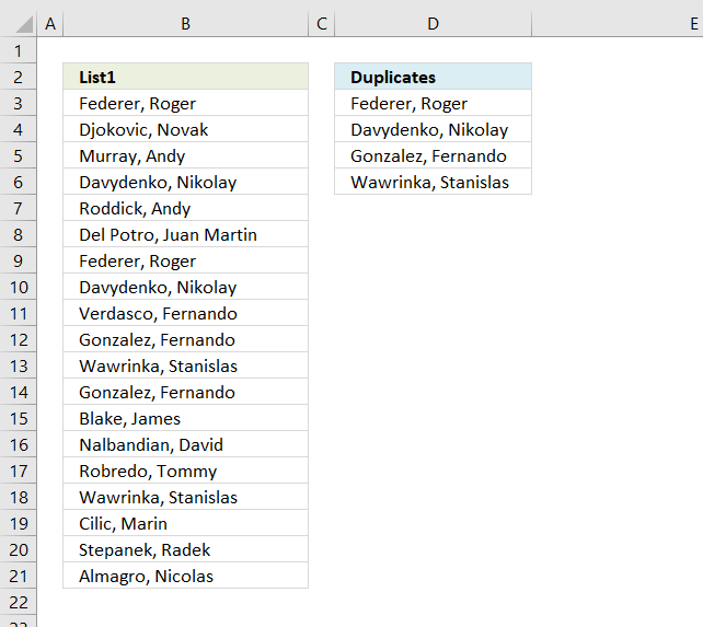
The array formula in cell C2 extracts duplicate values from column A. Only one duplicate of each value is displayed […]
This article demonstrates formulas and Excel tools that extract duplicates based on three conditions. The first and second condition is […]
Excel categories
Leave a Reply
How to comment
How to add a formula to your comment
<code>Insert your formula here.</code>
Convert less than and larger than signs
Use html character entities instead of less than and larger than signs.
< becomes < and > becomes >
How to add VBA code to your comment
[vb 1="vbnet" language=","]
Put your VBA code here.
[/vb]
How to add a picture to your comment:
Upload picture to postimage.org or imgur
Paste image link to your comment.