Extract specific word based on position in cell value
Whether you're cleaning up imported data, parsing product names, or building dynamic spreadsheets, mastering text manipulation in Excel can save you hours of manual editing. From simple tasks like extracting the first word in a cell to more advanced techniques like using recursive LAMBDA functions to substitute multiple values, Excel gives you a toolbox — if you know how to use it.
In this guide, I’ll walk through practical, real-world examples including:
- How to extract the first, n-th, or last word in a text string
- Methods to return a warning if the word is missing
- How to pull out the last letter or the last number from a cell
- Techniques to replace part of a formula across multiple cells
- Ways to substitute multiple text strings using both built-in Excel 365 functions and custom user-defined functions (UDFs)
Whether you're using classic Excel or taking advantage of the newest features in Excel 365, this guide has something for everyone who works with messy or structured text.
Let’s dive in!
Table of Contents
- Extract first word in cell value
- Extract the first word in cell - return warning if not found
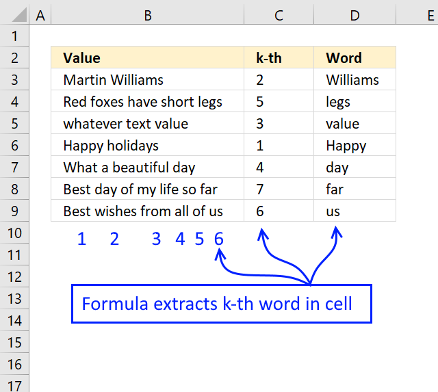
- Extract n-th word in cell value
- Extract n-th word in cell value - Excel 365
- Extract the last word
- Extract the last letter
- Extract the last number
- How to replace part of formula in all cells
- Substitute multiple text strings - Excel 365 recursive LAMBDA function
- Substitute multiple text strings - UDF
1. Introduction
Why extract the first word in a cell value?
To isolate names, titles, or categories from longer text strings. For example, "Mr. John Smith" to "Mr.". Useful when sorting, grouping, or filtering data based on the leading word. It helps standardize entries for lookup tables or drop-down lists.
Why extract the last word in a cell value?
Often used to capture key qualifiers or suffixes. For example, "Order #123 Delivered" to "Delivered". It helps identify status, locations, or designations that come last in descriptions. Can be useful in reports and summaries to highlight final keywords.
Why extract the last letter?
To determine codes or categories marked by a trailing character. For example, "Zone7B" to "B".
Why extract the last number?
To pull the most relevant or recent numerical data from a string. For example, "Invoice #2023-154" to "154".
Why extract the n-th word in a cell value?
There are many reasons, one can be: To break down structured text into components. For example, "City State Zip" to "State".
Why replace part of formula in all cells?
It saves time and avoids manual edits when updating worksheet formulas.
Why substitute strings in Excel?
There are many reasons, one can be: It enables batch corrections and improvements in data quality.
2. Extract first word in cell value
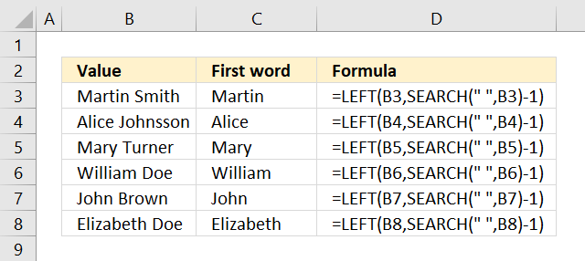
The formula in cell C3 grabs the first word in B3 using a blank as the delimiting character.
The SEARCH function looks for a "space" character in cell B3 and returns 7, if you want to use a different delimiting character change the first argument in the SEARCH function.
We don't need the space character so we subtract the number returned from the SEARCH function with 1.
The LEFT function then extracts the first word in cell B3 using the calculated number.
2.1 Explaining formula
Step 1 - Find string in value
The SEARCH function returns a number representing the position of character at which a specific text string is found reading left to right.
SEARCH(find_text,within_text, [start_num])
SEARCH(" ", B3)-1
becomes 7-1 and equals 6.
Step 2 - Extract string based on position
The LEFT function extracts a given number of characters always starting from the left.
LEFT(text, [num_chars])
LEFT(B3, SEARCH(" ", B3)-1)
becomes
LEFT(B3, 6)
becomes
LEFT("Martin Smith", 6)
and returns "Martin" in cell C3.
3. Extract the first word in cell - return warning if not found
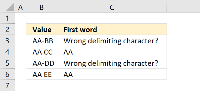
The following formula warns if the delimiting character is not found.
The SEARCH function returns #VALUE error if the delimiting character is not found. The COUNT function counts how many numbers are in a cell or cell range, it also ignores errors that come in handy in this case.
The COUNT function returns 0 (zero) in cell B3 and the IF function interprets that as a FALSE. The third argument in the IF function is returned "Wrong delimiting character?".
3.1 Explaining formula
Step 1 - Find position of character
The SEARCH function returns a number representing the position of character at which a specific text string is found reading left to right.
SEARCH(find_text,within_text, [start_num])
SEARCH(" ",B3)-1
becomes
SEARCH(" ","AA-BB")-1
becomes
#N/A! -1 and returns #N/A!.
Step 2 - Extract string from value
The LEFT function extracts a given number of characters always starting from the left.
LEFT(text, [num_chars])
LEFT(B3,SEARCH(" ",B3)-1)
becomes
LEFT(B3,#N/A!)
and returns #N/A!
Step 3 - Count numbers
The COUNT function counts all numerical values in an argument, it allows you to have up to 255 arguments.
COUNT(SEARCH(" ",B3))
becomes
COUNT(#N/A!)
and returns 0 (zero).
Step 4 - Show warning if the character is not found
The IF function returns one value if the logical test is TRUE and another value if the logical test is FALSE.
IF(logical_test, [value_if_true], [value_if_false])
IF(COUNT(SEARCH(" ",B3)), LEFT(B3,SEARCH(" ",B3)-1),"Wrong delimiting character?")
becomes
IF(0, LEFT(B3,SEARCH(" ",B3)-1),"Wrong delimiting character?")
and returns "Wrong delimiting character?" in cell C3.
Get Excel *.xlsx file
Extract first word in cell.xlsx
4. Extract n-th word in the cell value
Formula in cell D3:
I was inspired by Rick Rothstein's comment from the year 2012 when I made this formula.
If your words are longer than 200 characters change each instance of 200 in the formula above to a higher value.
The delimiting character is a blank (space character). Make sure you change that in the formula if the cell value contains a different string delimiting character.
Explaining the formula in cell C3
Step 1 - Delete leading and trailing spaces
The TRIM function deletes all blanks (space characters) except single blanks between strings in a cell value.
TRIM(B3) returns "Martin Williams".
Step 2 - Replace remaining spaces
The SUBSTITUTE function replaces each space character in the cell value to 200 space characters. The REPT function repeats the space character 200 times.
SUBSTITUTE(TRIM(B3)," ",REPT(" ",200))
becomes
SUBSTITUTE("Martin Williams"," "," ")
and returns "Martin Williams". (I have shortened the string for obvious reasons.)
Step 3 - Extract values
The MID function returns characters from the middle of a text string based on a start character and a number representing the length.
MID(SUBSTITUTE(TRIM(B3)," ",REPT(" ",200)), (C3-1)*200+1, 200)
becomes
MID("Martin Williams", (C3-1)*200+1, 200)
becomes
MID("Martin Williams", 201, 200)
and returns " Williams".
Step 4 - Once again delete leading and trailing spaces
Lastly, the TRIM function removes all blanks (space characters) except single blanks between strings in a cell value.
TRIM(MID(SUBSTITUTE(TRIM(B3)," ",REPT(" ",200)), (C3-1)*200+1, 200))
becomes
TRIM(" Williams")
and returns "Williams" in cell D3.
5. Extract n-th string in cell value - Excel 365

Excel 365 formula in cell D3:
5.1 Explaining formula
Step 1 - Split strings in value
The TEXTSPLIT function splits a string into an array based on delimiting values.
Function syntax: TEXTSPLIT(Input_Text, col_delimiter, [row_delimiter], [Ignore_Empty])
TEXTSPLIT(B3,," ",TRUE)
becomes
TEXTSPLIT("Martin Williams",," ",TRUE)
and returns
{"Martin"; "Williams"}.
Step 2 - Get k-th string in array
The INDEX function returns a value or reference from a cell range or array, you specify which value based on a row and column number.
Function syntax: INDEX(array, [row_num], [column_num])
INDEX(TEXTSPLIT(B3,," ",TRUE),C3)
becomes
INDEX({"Martin"; "Williams"},2)
and returns "Williams".
5.2 Get Excel *.xlsx file
Extract k-th word in cell.xlsx
6. Extract the last word
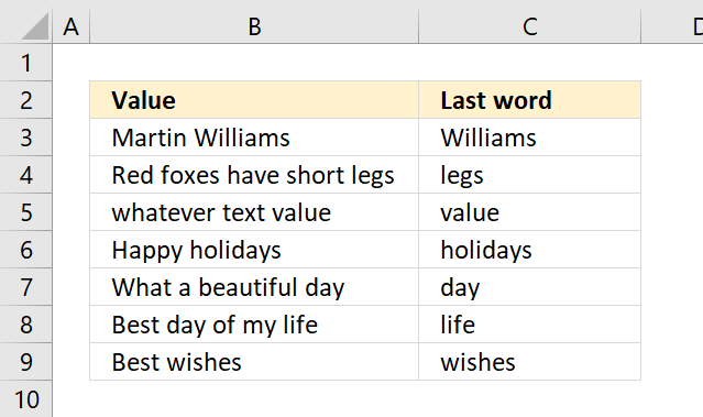
The formula demonstrated above in cell range C3:C9 extracts the last word from an adjacent cell in column B.
I was inspired by Rick Rothstein's comment from the year 2012 when I made this formula.
If your words are longer than 200 characters change each instance of 200 in the formula above to a higher value.
The delimiting character is a blank (space character). Make sure you change that if the cell value contains a different string delimiting character.
6.1 Explaining the formula in cell C3
Step 1 - Repeat space character 200 times
The REPT function repeats a specific text a chosen number of times.
REPT(text, number_times)
REPT(" ", 200)
returns 200 space characters concatenated.
Step 2 - Substitute space character with 200 space characters
The SUBSTITUTE function replaces each blank in the cell value to 200 blanks.
SUBSTITUTE(B3," ",REPT(" ",200))
becomes
SUBSTITUTE("Martin Williams"," "," ")
and returns "Martin Williams".
(I have shortened the string for obvious reasons.)
Step 3 - Extract 200 characters from right
The RIGHT function extracts the 200 characters starting from the right.
RIGHT(text,[num_chars])
RIGHT(SUBSTITUTE(B3," ",REPT(" ",200)), 200)
becomes
RIGHT("Martin Williams", 200)
and returns " Williams". All space characters are not shown for obvious reasons.
Step 4 - Remove leading space characters
The TRIM function removes all leading and trailing spaces in a string or cell value.
TRIM(RIGHT(SUBSTITUTE(B3, " ", REPT(" ", 200)), 200))
becomes
TRIM(" Williams")
and returns "Williams" in cell C3.
7. Extract the last letter

The formula in cell D3 extracts the last letter from characters in cell B3, the value contains letters, numbers, and other random characters.
Array formula in cell D3:
7.1 How to enter an array formula

The image above shows a leading curly bracket, the formula is too large to display the trailing curly bracket, however, it is there. They appear automatically when you follow the steps below.
- Copy the array formula above.
- Double press with the left mouse button on cell D3, a prompt appears.
- Paste it to cell C3, shortcut keys are CTRL + v.
- Press and hold CTRL + SHIFT keys simultaneously.
- Press Enter once.
- Release all keys.
The formula bar shows a beginning and ending curly bracket, don't enter these characters yourself.
7.2 Explaining formula
Step 1 - Search for all letters
The SEARCH function returns a number representing the position of character at which a specific text string is found reading left to right. It is not a case-sensitive search.
SEARCH(find_text,within_text, [start_num])
SEARCH({"a"; "b"; "c"; "d"; "e"; "f"; "g"; "h"; "i"; "j"; "k"; "l"; "m"; "n"; "o"; "p"; "q"; "r"; "s"; "t"; "u"; "v"; "w"; "x"; "y"; "z"}, B3)
returns {10; #VALUE!; ... ; #VALUE!}
Step 2 - Replace error values with blanks
The MAX function can't handle error values, we must take care of them. The IFERROR function can replace error values with a given value.
IFERROR(value, value_if_error)
IFERROR(SEARCH({"a"; "b"; "c"; "d"; "e"; "f"; "g"; "h"; "i"; "j"; "k"; "l"; "m"; "n"; "o"; "p"; "q"; "r"; "s"; "t"; "u"; "v"; "w"; "x"; "y"; "z"}, B3), "")
becomes
IFERROR({10; #VALUE!; ... ; #VALUE!}, "")
and returns
{10; ""; ...; ""}.
Step 3 - Calculate the largest number in the array
The MAX function returns the largest number in a cell range or array.
MAX(IFERROR(SEARCH({"a"; "b"; "c"; "d"; "e"; "f"; "g"; "h"; "i"; "j"; "k"; "l"; "m"; "n"; "o"; "p"; "q"; "r"; "s"; "t"; "u"; "v"; "w"; "x"; "y"; "z"}, B3), ""))
becomes
MAX({10; ... ; 16; ""; ""; ""; 4; ""; ""; ""})
and returns 16.
Step 4 - Extract the last letter
The MID function returns a substring from a string based on the starting position and the number of characters you want to extract.
MID(text, start_num, num_chars)
MID(B3, MAX(IFERROR(SEARCH({"a"; "b"; "c"; "d"; "e"; "f"; "g"; "h"; "i"; "j"; "k"; "l"; "m"; "n"; "o"; "p"; "q"; "r"; "s"; "t"; "u"; "v"; "w"; "x"; "y"; "z"}, B3), "")), 1)
becomes
MID("12 Wi llia3 3m s2 ", 16, 1)
and returns "s" in cell D3.
8. Extract the last digit in a cell

The image above demonstrates an array formula in cell D3 that extracts the last digit in cell B3.
Array formula in cell D3:
8.1 Explaining formula
Step 1 - Search for all digits
The SEARCH function returns a number representing the position of character at which a specific text string is found reading left to right. It is not a case-sensitive search.
SEARCH(find_text,within_text, [start_num])
SEARCH({0; 1; 2; 3; 4; 5; 6; 7; 8; 9}, B3)
becomes
SEARCH({0; 1; 2; 3; 4; 5; 6; 7; 8; 9}, "12?Wi:llia3 3m_s ")
and returns
{#VALUE!; 1; 2; ... ; #VALUE!}.
Step 2 - Replace error values with blanks
The IFERROR function can replace error values with a given value.
IFERROR(value, value_if_error)
IFERROR(SEARCH({0; 1; 2; 3; 4; 5; 6; 7; 8; 9}, B3), ""))
becomes
IFERROR({#VALUE!; 1; 2; ...; #VALUE!})
and returns
{""; 1; 2; 11; ... ; ""}.
Step 3 - Calculate the largest number in the array
The MAX function returns the largest number in a cell range or array.
MAX(IFERROR(SEARCH({0; 1; 2; 3; 4; 5; 6; 7; 8; 9}, B3), ""))
becomes
MAX({""; 1; 2; 11; ... ; ""})
and returns 11.
Step 4 - Extract last letter
The MID function returns a substring from a string based on the starting position and the number of characters you want to extract.
MID(text, start_num, num_chars)
MID(B3, MAX(IFERROR(SEARCH({0; 1; 2; 3; 4; 5; 6; 7; 8; 9}, B3), "")), 1)
becomes
MID("12?Wi:llia3 3m_s ", 11, 1)
and returns "s" in cell D3.
8.2 Get Excel *.xlsx file
Extract last word in cell.xlsx
9. How to replace part of formula in all cells
This section explains how to substitute part of a formula across all cells in a worksheet. It is easier than you think, no VBA programming or formulas are needed.
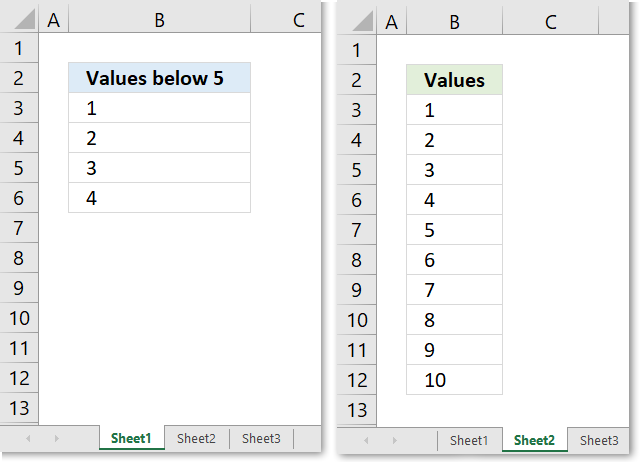
The picture above demonstrates a simple example, the formula in cell B3 gets values below 5 from sheet 2 cell range B3:B12.
Array formula in cell B3
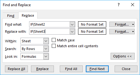
I will now show you how to replace Sheet2 with Sheet3 in formulas, in all cells in Sheet1. Simply press CTRL and H to open the Find and Replace dialog box.
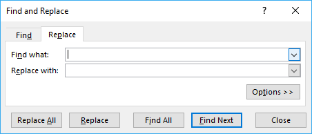
Press with left mouse button on the "Options" button to see all settings.
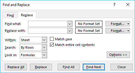
Here you have the option to
- Search the entire workbook or just the active worksheet. I want to search the active worksheet so I change nothing.
- Match entire cell contents. Deselect the check box, I want to match specific strings in formulas.
Press with left mouse button on in field "Find what:" and type Sheet2. Now press with left mouse button on in field "Replace with:" and type Sheet3, then press with left mouse button on "Replace All" button.
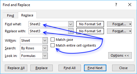
This will find all instances of Sheet2 in all cells and replace them with Sheet3.
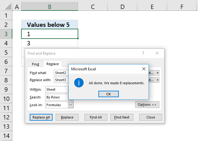
Press with left mouse button on the "OK" button and then the "Close" button.
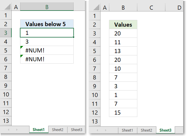
The array formula in cell B3 (Sheet1) changes to:
Recommended article
Recommended articles
Today I'll show you how to search all Excel workbooks with file extensions xls, xlsx and xlsm in a given folder for a […]
9.1 Replace part of formula in a specific cell range
Simply select the cell range, press CTRL + H to open the Find and Replace dialog box.
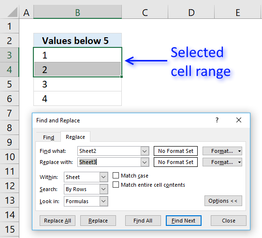
The "Find and Replace" action will now be applied to cell range B3:B4.
9.2 Replace n:th instance
Array formula in cell B3 (Sheet1)
To replace only the first instance of a specific search string in the formula simply include more characters so it makes the search string unique.
Example, you want to replace Sheet2 with Sheet3 but only the first instance found in the formula.
Press CTRL + H to open the Find and Replace dialog box.
Don't forget to add the included characters in the "Replace with: " field as well.
String IF(Sheet2 is found in only one location in each cell, this will replace only the first instance of Sheet2.
10. Substitute multiple text strings - Excel 365 recursive LAMBDA function
The SUBSTITUTE and REPLACE functions can only handle one string, the next two sections demonstrate two ways to handle more than one pair of values.
- An Excel 365 recursive LAMBDA function.
- A User-Defined Function (UDF) allows you to substitute multiple text strings with new text strings.

This example demonstrates a formula that iterates through all values in cell range E3:F4 in order to substitute specific values in cell B3 with new values.
The SUBSTITUTE function allows you to substitute one value with another value, however, this formula lets you substitute (almost) any number of values.
Excel 365 LAMBDA function in Name Manager:
The LAMBDA function is named SUBSTR in the Name Manager.
Excel 365 formula in cell C3:
10.1 Explaining LAMBDA formula
Step 1 - Get old string
The INDEX function returns a value or reference from a cell range or array, you specify which value based on a row and column number.
Function syntax: INDEX(array, [row_num], [column_num])
INDEX(sub,n,1)
sub is a variable, in this example cell reference $E$3:$F$4
n is a number, representing the number of rows in cell reference $E$3:$F$4
1 is the first column in cell reference $E$3:$F$4
Step 2 - Get new string
The INDEX function returns a value or reference from a cell range or array, you specify which value based on a row and column number.
Function syntax: INDEX(array, [row_num], [column_num])
INDEX(sub,n,2)
sub is a variable, in this example cell reference $E$3:$F$4
n is a number, representing the number of rows in cell reference $E$3:$F$4
2 represents the second column in cell reference $E$3:$F$4
Step 3 - Substitute given values
The SUBSTITUTE function replaces a specific text string in a value. Case sensitive.
Function syntax: SUBSTITUTE(text, old_text, new_text, [instance_num])
SUBSTITUTE(str,INDEX(sub,n,1),INDEX(sub,n,2))
Step 4 - Make this formula recursive
The LAMBDA function is named SUBSTR in the name manager. We can call this named formula again until all values have been used.
SUBSTR(str,sub,n)
The SUBSTR function has three arguments:
- str - the string
- sub - the values to substitute
- n - the number of rows (or substitute pairs in cell ref $E$3:$F$4
SUBSTR(SUBSTITUTE(str,INDEX(sub,n,1),INDEX(sub,n,2)),sub,n-1)
str => SUBSTITUTE(str,INDEX(sub,n,1),INDEX(sub,n,2))
sub => sub (no change)
n => n - 1
n is keeping track of the row number. By subtracting one for each iteration the changes and a new pair of substitute values are processed.
Step 5 - Control the recursive formula
The IF function returns one value if the logical test is TRUE and another value if the logical test is FALSE.
Function syntax: IF(logical_test, [value_if_true], [value_if_false])
The IF function returns the string str if n is equal to 0 (zero), however, it calls the SUBSTR function again if not. This step is repeated like a loop until n is equal to 0 (zero).
IF(n=0,str,SUBSTR(SUBSTITUTE(str,INDEX(sub,n,1),INDEX(sub,n,2)),sub,n-1))
Step 6 - Create the LAMBDA function and define the parameters
The LAMBDA function build custom functions without VBA, macros or javascript.
Function syntax: LAMBDA([parameter1, parameter2, …,] calculation)
LAMBDA(str,sub,n,IF(n=0,str,SUBSTR(SUBSTITUTE(str,INDEX(sub,n,1),INDEX(sub,n,2)),sub,n-1)))
10.2 Name LAMBDA function in the Name Manager
- Go to tab "Formulas" on the ribbon.
- Press the left mouse button on the "Name Manager" button.
A dialog box opens. - Press with left mouse button on the "New..." button. A new dialog box appears.
- Name the function.

- Paste the LAMBDA formula in the "Refers to:" field.
- Press with left mouse button on OK button.
You are now ready to use the named LAMBDA function. Select an empty cell. Type =SUBSTR( and the arguments, don't forget the ending parentheses. Press Enter.
11. How to use the User Defined Function

You may have as many strings as you like, there is really no limit. The image above shows the UDF in cell C3 using strings from E3:E4 and F3:F4.
Formula in cell C3:
The UDF will not appear and work yet until you have copied the code below to a module in your workbook. There are instructions below.
Got it working? Now copy cell C3 and paste to cells below, the first argument contains relative cell references meaning they will change automatically when you copy and paste cell C3 to cells below.
The second and third argument are absolute cell references, they contain dollar signs meaning they are locked to cell range $D$2:$D$3 and $E$2:$E$3. These cell references will not change when you copy cell C3 and paste to the cells below.
11.1 User Defined Syntax
SubstituteMultiple(text As String, old_text As Range, new_text As Range)
11.2 Arguments
| text | Required. A cell reference to a cell containing the text you want to manipulate. |
| old_text | Required. A cell reference to one or many cells containing strings you want to replace. |
| new_text | Required. A cell reference to one or many cells containing strings you want instead. |
11.3 VBA code
'Name function and dimension argument variables and declare their data types
Function SubstituteMultiple(text As String, old_text As Range, new_text As Range)

'Dimension variable and declare data type
Dim i As Single

'Iterate through cells in argument old_text
For i = 1 To old_text.Cells.Count

    'Replace strings in value based on variable i
    Result = Replace(LCase(text), LCase(old_text.Cells(i)), LCase(new_text.Cells(i)))

    'Save manipulated value to variable text
    text = Result
Next i

'Return value stored in variable Result to worksheet
SubstituteMultiple = Result
End Function
11.4 Where to put the code?
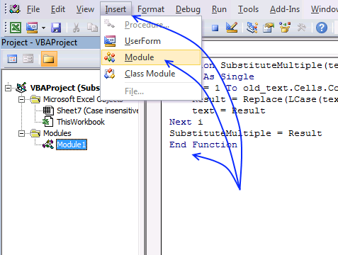
- Copy above VBA code.
- Go to the Visual Basic Editor (Shortcut keys Alt + F11).
- Press with left mouse button on Insert on the top menu.
- Press with left mouse button on Module to create a module in your workbook. A module named module1 appears in the Project Explorer.
- Paste code to module.
- Exit VB Editor
11.5 How to save a macro-enabled workbook
Extract category
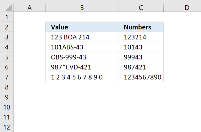
Working with numbers in Excel can be deceptively tricky, especially when they're embedded within text or need to be formatted […]
Excel categories
11 Responses to “Extract specific word based on position in cell value”
Leave a Reply
How to comment
How to add a formula to your comment
<code>Insert your formula here.</code>
Convert less than and larger than signs
Use html character entities instead of less than and larger than signs.
< becomes < and > becomes >
How to add VBA code to your comment
[vb 1="vbnet" language=","]
Put your VBA code here.
[/vb]
How to add a picture to your comment:
Upload picture to postimage.org or imgur
Paste image link to your comment.
Do you have a version that is case sensitive?
Ari,
Function SubstituteMultiple(text As String, old_text As Range, new_text As Range) Dim i As Single For i = 1 To old_text.Cells.Count Result = Replace(text, old_text.Cells(i), new_text.Cells(i)) text = Result Next i SubstituteMultiple = Result End FunctionGreat solution, thanks!
this is best solution from whole google search results , Thanks very much.
but there is little difference within Substitute and SubstituteMultiple:
Substitude Multiple Changes Texts UperCase symbols To LowCase, can someone help how to fix this?
Zurab Lomidze,
Thank you. Try this udf, it is case sensitive.
Function SubstituteMultipleCS(text As String, old_text As Range, new_text As Range) Dim i As Single For i = 1 To old_text.Cells.Count Result = Replace(text, old_text.Cells(i), new_text.Cells(i)) text = Result Next i SubstituteMultipleCS = Result End FunctionGood article. Often, I need to select up to a delimiter character or the whole cell contents, whichever is applicable.
Suppose cell A2 = "ABC|DEF", cell A3 = "Words". And, in this case, my delimiter is the vertical bar or pipe character "|".
=left(A2,search("|",A2 & "|")-1)For cell A2, I append a vertical bar, so what I'm searching is actually the string "ABC|DEF|". The search will still find the first vertical bar (position 4) and then subtract 1 for the left function, producing "ABC".
If we used cell A3 instead of A2, appending the vertical bar to the string "Words" would give us "Words|". The position returned by the search function is 6, and subtracting 1 from this (now 5) gives us the length of the string, so the left function gets the original string.
Whether you use this approach or not is largely dependent upon what you're trying to produce. This covers most of my use cases, and when I discovered it, it simplified lots of my coding (SQL and Excel for sure).
Thank you Jack for your comment.
Very useful if a cell does not contain the specified delimiting character at all.
=LEFT(B3,SEARCH(" ",B3&" ")-1)
You saved my day, Thanks
omgness, thank you so much
Great post, Oscar; I use this function all the time. A problem I need help with is that the replacement keeps looping through my replaced text. For example, I have a "Remarks" column with a cell containing "A,B". Each character represents an index item from a multi-column table elsewhere.
A = ALMOND BERRY
B = BLUE COCONUT
Here is the formula I'm running:
=SubstituteMultiple("A,B",{"A";"B"},{"ALMOND BERRY";"BLUE COCONUT"})
I want to produce the following result:
"ALMOND BERRY,BLUE COCONUT"
However, the following results from the SubstituteMultiple UDF:
"ALMOND BLUE COCONUTERRY,BLUE COCONUT"
The problem is that the index character is an alphabetical character that appears in the second of the replacement phrase, thus causing a replacement loop on the second term in the "new_text".
What are your thoughts? Thanks for your effort.
This is great. I don't know why excel doesn't have inbuilt functionality for multiple substitutes (in the vein of IF vs IFS, or the above)
Is anyone able to help modify the above so it can handle an array as the Text argument? I would like the function to remove all instances of Old_text from an entire column.
Thanks in advance!