Get date ranges from a schedule
This article demonstrates ways to extract names and corresponding populated date ranges from a schedule using Excel 365 and earlier Excel versions.
Table of Contents
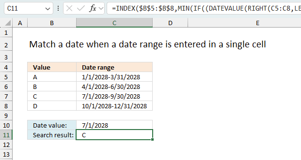
1. Get date ranges from a schedule - Excel 365
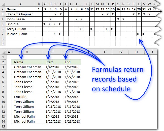
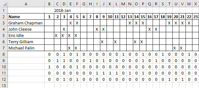
The following formulas extract names and date ranges from the schedule in sheet1, the schedule has dates in row 2 and names column A.
The "x" indicates populated days. The formulas use the "x" to extract the correct name and the corresponding dates. Note that there may be multiple date ranges in the schedule for the same person.
Excel 365 dynamic array formula in cell B3:
Excel 365 dynamic array formula in cell C3:
Excel 365 dynamic array formula in cell D3:
1.1 Explaining formula in cell B3
The formulas in cell C3 and D3 are similar to the formula in cell B3, they extract start and end dates instead of names.
Step 1 - Compare cell ranges and check if values are not equal
The less than and larger than signs are logical operators, they return TRUE or FALSE which are boolean values. The less than and the greater than signs combined means "not equal to"
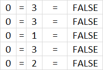
Sheet1!B3:NA7<>Sheet1!C3:NB7
becomes
{0,0,0,"X", ... ,0}<>{0,0,"X","X", ... ,0}
These are big arrays, and I have shortened them.
{0,0,0,"X", ... ,0}<>{0,0,"X","X", ... ,0}
returns
{FALSE,FALSE,TRUE,FALSE, ... , FALSE}

Note that the cell references are not perfectly aligned, the last cell reference (red) is offset one cell to the right. This technique lets us pinpoint when a populated cell range begins and ends.

The way comparing cell ranges works is that a cell in one cell range is compared to the corresponding cell in the second cell range. For example, cell B2 is compared to C2 and only C2. Cell B3 is compared to cell C3 and so on.
Step 2 - Check if cells are empty
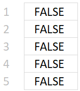
The equal sign is also a logical operator, the following part cheks if a cell is empty "".
Sheet1!B3:NA7=""
becomes
{"","","","X", ... ,""}=""
and returns
{TRUE,TRUE,TRUE, FALSE, ... ,TRUE}
Step 3 - Multiply arrays
The asterisk lets you multiply numbers and boolean values in an Excel formula. This lets you create AND logic between boolean values meaning both values must be TRUE to return TRUE.
TRUE * TRUE = TRUE (1)
TRUE * FALSE = FALSE (0)
FALSE * TRUE = FALSE (0)
FALSE * FALSE = FALSE (0)
Excel converts the result to the boolean values numerical equivalents.
TRUE = 1
FALSE = 0
(Sheet1!B3:NA7<>Sheet1!C3:NB7)*(Sheet1!B3:NA7="")
becomes
{FALSE,FALSE,TRUE,FALSE, ... , FALSE}*{TRUE,TRUE,TRUE, FALSE, ... ,TRUE}
and returns
{0,0,1,0, ... ,0}
Step 4 - Replace with names from column A
The IF function returns one value if the logical test is TRUE and another value if the logical test is FALSE.
Function syntax: IF(logical_test, [value_if_true], [value_if_false])
IF((Sheet1!B3:NA7<>Sheet1!C3:NB7)*(Sheet1!B3:NA7=""),Sheet1!A3:A7,"")
becomes
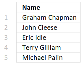
IF({0,0,1,0, ... ,0}, {"Graham Chapman"; "John Cleese"; "Eric Idle"; "Terry Gilliam"; "Michael Palin"},"")
and returns
{"","","Graham Chapman", ... ,""}
Step 5 - Rearrange values to a single column layout
The TOCOL function rearranges values in 2D cell ranges to a single column.
Function syntax: TOCOL(array, [ignore], [scan_by_col])
TOCOL(IF((Sheet1!B3:NA7<>Sheet1!C3:NB7)*(Sheet1!B3:NA7=""),Sheet1!A3:A7,""))
becomes
TOCOL({"","","Graham Chapman", ... ,""})
and returns
{"";"";"Graham Chapman"; ... ;""}
Note that the semicolons changed to commas. They are delimiting characters in an array, you may have other characters as they are based on the regional settings of your computer.
Step 6 - Check if cells are not empty
This step is to create a logical test that is then used in the next step to filter out empty values.
TOCOL(IF((Sheet1!B3:NA7<>Sheet1!C3:NB7)*(Sheet1!B3:NA7=""),Sheet1!A3:A7,""))<>""
becomes
{"";"";"Graham Chapman"; ... ;""}<>""
and returns
{FALSE;FALSE;TRUE; ... ;FALSE}
Step 7 - Filter out empty values
The FILTER function extracts values/rows based on a condition or criteria.
Function syntax: FILTER(array, include, [if_empty])
FILTER(TOCOL(IF((Sheet1!B3:NA7<>Sheet1!C3:NB7)*(Sheet1!B3:NA7=""),Sheet1!A3:A7,"")),TOCOL(IF((Sheet1!B3:NA7<>Sheet1!C3:NB7)*(Sheet1!B3:NA7=""),Sheet1!A3:A7,""))<>""))
becomes
FILTER({"";"";"Graham Chapman"; ... ;""},Sheet1!A3:A7,"")),{FALSE;FALSE;TRUE; ... ;FALSE})
and returns
{"Graham Chapman"; "Graham Chapman"; "Graham Chapman"; ... ; "Michael Palin"}
Step 8 - Shorten formula
The LET function lets you name intermediate calculation results which can shorten formulas considerably and improve performance.
Function syntax: LET(name1, name_value1, calculation_or_name2, [name_value2, calculation_or_name3...])
FILTER(TOCOL(IF((Sheet1!B3:NA7<>Sheet1!C3:NB7)*(Sheet1!B3:NA7=""),Sheet1!A3:A7,"")),TOCOL(IF((Sheet1!B3:NA7<>Sheet1!C3:NB7)*(Sheet1!B3:NA7=""),Sheet1!A3:A7,""))<>""))
x - Sheet1!B3:NA7
y - Sheet1!C3:NB7
w - TOCOL(IF((x<>y)*(x=""),Sheet1!A3:A7,""))
LET(x,Sheet1!B3:NA7,y,Sheet1!C3:NB7,w,TOCOL(IF((x<>y)*(x=""),Sheet1!A3:A7,"")),FILTER(w,w<>""))
1.2 Get Excel *.xls file
2. Get date ranges from a schedule - earlier Excel versions
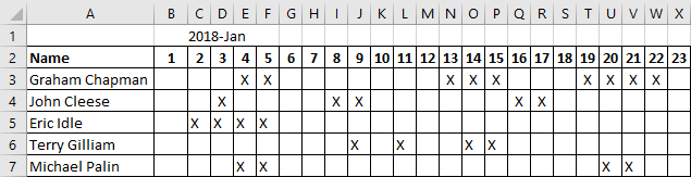
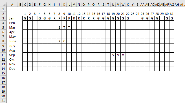
The above picture shows you two formulas that extract names (column B) and date ranges (column C and D) based on a cross-reference schedule.
The schedule has dates in row 2, however, the cell is formatted to show only the day number.
Names are in column A and there are no duplicate names. An X indicates that a date is selected for the given person, multiple x's in a sequence is a date range.
The array formula in cell B3 returns the correct number names needed to return all date ranges:
Array formula in cell C3:
Array formula in cell D3:
- Sheet1!$A$3:$A$7 is the cell reference to the names in the schedule.
- Sheet1!$B$3:$AA$7 and Sheet1!$C$3:$AB$7 are a cell reference to the X's in the schedule.
Two are needed for the formula to count the number of date ranges.
Note! The cell refs have the same size, however, the latter is offset by one column.
How to enter an array formula
To enter an array formula, type the formula in cell B3 then press and hold CTRL + SHIFT simultaneously, now press Enter once. Release all keys.
 The formula bar now shows the formula with a beginning and ending curly bracket telling you that you entered the formula successfully.
Don't enter the curly brackets yourself, they appear automatically.
Explaining the formula in cell B3
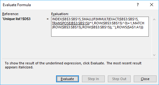
Use "Evaluate Formula" on tab "Formula" on the ribbon to go through the steps.
Step 1 - Count previous values
COUNTIF($B$2:B2,Sheet1!$A$3:$A$7)
becomes
COUNTIF("Name", {"Graham Chapman"; "John Cleese"; "Eric Idle"; "Terry Gilliam"; "Michael Palin"})
and returns {0;0;0;0;0}. None of the names have been displayed in cells above, remember that I am right now showing the calculation steps in cell B3.
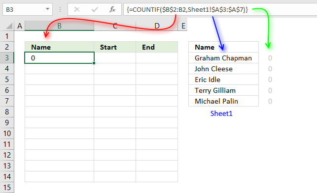
As soon as the first name has been displayed the same number of times as it has date ranges the formula continues to the second name.
We are now going to count how many date ranges there is in the schedule per row.
Step 2 - Calculate where a cell value changes in a row
To count date ranges the formula needs to compare a cell with the next. To be able to compare all values in one calculation I use two cell ranges. The last cell range has the same size as the first, however, it is offset one column to the right.
(Sheet1!$B$3:$AA$7<>Sheet1!$C$3:$AB$7)*1
becomes
{0, 0, 1, 0, 1, 0, 0, 0, 0, 0, 0, 1, 0, 0, 1, 0, 0, 1, 0, 0, 0, 1, 0, 0, 0, 0;0, 1, 1, 0, 0, 0, ... , 0}
Part of the array is displayed in cell range B8:X12 in picture below.
Step 3 - Sum values per row
The amazing MMULT function allows you to sum numbers in an array per row or column. The earlier calculation step created an array that shows when a cell has a different value compared to the next cell.
That makes the array show when a date range starts and ends, to be able to count date ranges we must divide the sum of each row with 2.
(MMULT((Sheet1!$B$3:$AA$7 <> Sheet1!$C$3:$AB$7)*1, TRANSPOSE(COLUMN(Sheet1!$B$3:$AA$4)^0))/2)
becomes
({6; 6; 2; 6; 4}/2)
and returns {3; 3; 1; 3; 2}.
The array tells us that the first name has three date ranges, the second name has three date ranges and so on.
The image above shows that the first name has three date ranges, the second has 3, the third has 1, the fourth has 3, and the last name has 2 date ranges.
The calculation is correct.
Step 4 - Compare arrays
The number of names displayed must match the corresponding number of date ranges.
To do that I compare the arrays, if they are equal the logical expression returns TRUE. If not equal it returns FALSE.
COUNTIF($B$2:B2, Sheet1!$A$3:$A$7)=(MMULT((Sheet1!$B$3:$AA$7<>Sheet1!$C$3:$AB$7)*1, TRANSPOSE(COLUMN(Sheet1!$B$3:$AA$4)^0))/2)
 becomes
{0;0;0;0;0}={3; 3; 1; 3; 2}
and returns {FALSE; FALSE; FALSE; FALSE; FALSE}.
Step 5 - Find position of first name that is shown less times than there is corresponding date ranges
The MATCH function allows you to identify the position of a specific value in an array or cell range, if the third argument in the MATCH function is 0 (zero) meaning EXACT match.
MATCH(FALSE, COUNTIF($B$2:B2, Sheet1!$A$3:$A$7)=(MMULT((Sheet1!$B$3:$AA$7<>Sheet1!$C$3:$AB$7)*1, TRANSPOSE(COLUMN(Sheet1!$B$3:$AA$4)^0))/2), 0)
 becomes
MATCH(FALSE, {FALSE; FALSE; FALSE; FALSE; FALSE}, 0)
and returns 1.
Step 6 - Get the name
The INDEX function gets the first value in cell range Sheet1!$A$3:$A$7.
INDEX(Sheet1!$A$3:$A$7, MATCH(FALSE, COUNTIF($B$2:B2, Sheet1!$A$3:$A$7)=(MMULT((Sheet1!$B$3:$AA$7<>Sheet1!$C$3:$AB$7)*1, TRANSPOSE(COLUMN(Sheet1!$B$3:$AA$4)^0))/2), 0))
becomes
 INDEX(Sheet1!$A$3:$A$7, 1)
becomes
INDEX({"Graham Chapman"; "John Cleese"; "Eric Idle"; "Terry Gilliam"; "Michael Palin"}, 1)
and returns "Graham Chapman" in cell B3.
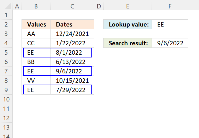
3. Extract dates from a cell block schedule
Sam asks:
One more question for the Calendar that you have set up above can we have a excel formula which will give us a below table
StarWk EndWk Name
1 2 G
4 6 G
7 15 R ... and so on
Question found here.
Answer:

The image above shows three different formulas that extract groups based on adjacent text names from a calendar, the calendar is shown in the top image. The only exception is a range that spans over at least two months, it will be divided into two date ranges.
Excel 365 dynamic array formula in cell B3:
The following formulas are for older Excel versions:
Array Formula in cell B3:
Array Formula in cell C3:
Formula in cell D3:
To enter an array formula, type the formula in a cell then press and hold CTRL + SHIFT simultaneously, now press Enter once. Release all keys.
The formula bar now shows the formula with a beginning and ending curly bracket telling you that you entered the formula successfully. Don't enter the curly brackets yourself.
Copy cell A2 and paste it down as far as needed.
Explaining formula in cell B3
Step 1 - Compare cell ranges
The less than and greater than signs combined returns TRUE if a cell is not equal to the next.
Sheet1!$C$3:$AG$14<>Sheet1!$B$3:$AF$14
becomes
{"G", "G", 0, ... I made the array shorter ... , 0}<>{0, "G", "G", ... , 0}
and returns
{TRUE, FALSE, TRUE, ... , FALSE}
Step 2 - Check if cell is not empty
Sheet1!$C$3:$AG$14<>""
returns
{TRUE, TRUE, FALSE, ... , FALSE}
Step 3 - Multiply arrays
(Sheet1!$C$3:$AG$14<>Sheet1!$B$3:$AF$14)* (Sheet1!$C$3:$AG$14<>"")
becomes
{TRUE, FALSE, TRUE, ... , FALSE}* {TRUE, TRUE, FALSE, ... , FALSE}
and returns
{1,0,0,... ,0}
Step 4 - Convert array into dates
The IF function has three arguments, the first one must be a logical expression. If the expression evaluates to TRUE then one thing happens (argument 2) and if FALSE another thing happens (argument 3). The following lines explain the logical expression:
IF((Sheet1!$C$3:$AG$14<>Sheet1!$B$3:$AF$14)* (Sheet1!$C$3:$AG$14<>""), DATE(2018, ROW($1:$12), Sheet1!$C$2:$AG$2), "")
becomes
IF({1,0,0,... ,0}, DATE(2018, ROW($1:$12), Sheet1!$C$2:$AG$2), "")
becomes
IF({1,0,0,... ,0}, DATE(2018, {1;2;3;4;5;6;7;8;9;10;11;12}, Sheet1!$C$2:$AG$2), "")
and returns
{43101,"","", ... ,""}
Step 5 - Extract dates
To be able to return a new value in a cell each I use the SMALL function to filter column numbers from smallest to largest.
The ROWS function keeps track of the numbers based on an expanding cell reference. It will expand as the formula is copied to the cells below.
SMALL(IF((Sheet1!$C$3:$AG$14<>Sheet1!$B$3:$AF$14)* (Sheet1!$C$3:$AG$14<>""), DATE(2018, ROW($1:$12), Sheet1!$C$2:$AG$2), ""), ROWS($A$1:A1))
becomes
SMALL({43101,"","", ... ,""}, ROWS($A$1:A1))
becomes
SMALL({43101,"","", ... ,""}, 1)
and returns 43101 (1/1/2018) in cell B3.
Array Formula in cell C3:
Copy cell B2 and paste it down as far as needed. I am not going to explain this formula, it is very similar to the one in cell B3.
Formula in cell D3:
Copy cell C2 and paste it down as far as needed.
Explaining formula in cell D3
Step 1 - Calculate month number from 1 to 12 based on date
The MONTH function extracts the month as a number from an Excel date.
MONTH(B3)
becomes
MONTH(1/1/2018)
becomes
MONTH(43101)
and returns 1.
Step 2 - Calculate day number based on date
The DAY function extracts the day as a number from an Excel date.
DAY(B3)
becomes
DAY(1/1/2018)
becomes
DAY(43101)
and returns 1.
Step 3 - Get text name based on month and day
The INDEX function returns a value based on a cell reference and column/row numbers.
INDEX(Sheet1!$C$3:$AG$14,MONTH(B3),DAY(B3))
becomes
INDEX(Sheet1!$C$3:$AG$14,1,1)
and returns "G" in cell D3.
4. Shift Schedule
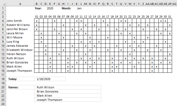
Hi Oscar, I have a cross reference table we use for shift scheduling. The x-axis is comprised of dates and the y is names. The table values indicate whether or not the employee is scheduled to work (i.e., filled or not).
Is there any way to pull a list of names in a canned daily report based on the date and whether the cell is filled? In other words, I want to look up the y-axis headers as opposed to the cross reference value.
Thanks, Geoff
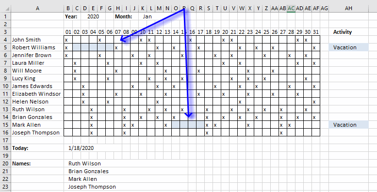
The image above demonstrates a schedule with dates on row 3, they are calculated automatically based on the selected year in cell D1 and month in K1.
You have to enter the names in column A and if they are scheduled for work (filled x) in the corresponding cells. Cell B18 returns the current date today and cell B20 and below return the names of the people that work that particular day.
Formula in cell B18:
Array formula in cell B20:
4.0.1 How to create an array formula
- Select cell B19
- Paste array formula in formula bar

- Press and hold CTRL + SHIFT
- Press Enter
4.0.2 How to copy array formula
- Select cell B20
- Copy (Ctrl + c)
- Select cell range B21:B26
- Paste (Ctrl + v)
4.1 Explaining array formula in cell B20
Step 1 - Find position of current date on row 3
This so we can extract the entire column in a later step. The MATCH function allows us to identify the position of a given value in an array or cell range.
The cell range must, however, have only one column or row. In other words, the cells must be horizontally or vertically arranged.
MATCH($B$18, $B$3:$AF$3, 0)
becomes
MATCH(40926, {40909, 40910, 40911, 40912, 40913, 40914, 40915, 40916, 40917, 40918, 40919, 40920, 40921, 40922, 40923, 40924, 40925, 40926, 40927, 40928, 40929, 40930, 40931, 40932, 40933, 40934, 40935, 40936, 40937, 40938, 40939}, 0)
and returns 18.
Excel date 40926 is found in the 18th position of cell range $B$1:$AF$1.
Step 2 - Extract values in a specific column
The INDEX function lets you extract a specific column based on a column number and a cell range to an array.
INDEX(cell_ref, row_num, [column_num], [area_num]
INDEX($B$4:$AF$14, 0, MATCH($B$18, $B$3:$AF$3, 0))
becomes
INDEX($B$4:$AF$14, 0, 18)
and returns the values in cell range S2:S14.
{0; 0; 0; 0; 0; 0; 0; 0; 0; "x"; "x"; "x"; "x"}
Step 3 - Identify which cells contain x
The equal sign compares each value in the array with x, if they match TRUe is returned and FALSE if not. TRUE and FALSE are boolean values.
INDEX($B$4:$AF$14, 0, MATCH($B$18, $B$3:$AF$3, 0))="x"
becomes
{0; 0; 0; 0; 0; 0; 0; 0; 0; "x"; "x"; "x"; "x"}="x"
and returns
{FALSE; FALSE; FALSE; FALSE; FALSE; FALSE; FALSE; FALSE; FALSE; TRUE; TRUE; TRUE; TRUE}
Step 4 - Replace TRUE with corresponding row number and FALSE with blanks
The IF function returns a value if the logical expression is TRUE and another value if FALSE. Since we are working with arrays the values returned are determined by the position of the value in the array.
IF(INDEX($B$4:$AF$14, 0, MATCH($B$18, $B$3:$AF$3, 0))="x", MATCH(ROW($A$4:$A$16), ROW($A$4:$A$16)), "")
becomes
IF({FALSE; FALSE; FALSE; FALSE; FALSE; FALSE; FALSE; FALSE; FALSE; TRUE; TRUE; TRUE; TRUE}, MATCH(ROW($A$4:$A$16), ROW($A$4:$A$16)), "")
becomes
IF({FALSE; FALSE; FALSE; FALSE; FALSE; FALSE; FALSE; FALSE; FALSE; TRUE; TRUE; TRUE; TRUE}, {1;2;3;4;5;6;7;8;9;10;11;12;13}, "")
and returns
{""; ""; ""; ""; ""; ""; ""; ""; ""; 10; 11; 12; 13}.
Step 5 - Extract the k-th smallest row number
The SMALL function allows you to extract a single value in each cell based on a row number.
SMALL(IF(INDEX($B$4:$AF$14, 0, MATCH($B$18, $B$3:$AF$3, 0))="x", MATCH(ROW($A$4:$A$16), ROW($A$4:$A$16)), ""), ROWS($A$1:A1))
becomes
SMALL({""; ""; ""; ""; ""; ""; ""; ""; ""; 10; 11; 12; 13}, ROWS($A$1:A1))
The ROWS function has a cell reference that changes when you copy the cell and paste to cells below, this is what makes the formula extract a new value in each cell.
SMALL({""; ""; ""; ""; ""; ""; ""; ""; ""; 10; 11; 12; 13},1)
and returns 10.
Step 6 - Get the name from column A based on a row number
The INDEX function lets you extract a value based on a cell range and a row and column number. Our cell range contains only one column so we can leave out the column number.
INDEX($A$4:$A$16, SMALL(IF(INDEX($B$4:$AF$14, 0, MATCH($B$18, $B$3:$AF$3, 0))="x", MATCH(ROW($A$4:$A$16), ROW($A$4:$A$16)), ""), ROWS($A$1:A1)))
Step 7 - Return blank if formula returns an error
The IFERROR function handles all errors so be careful if you use this function. If there is something else wrong you won't spot it because the IFERROR function returns a blank in that case as well.
IFERROR(INDEX($A$4:$A$16, SMALL(IF(INDEX($B$4:$AF$14, 0, MATCH($B$18, $B$3:$AF$3, 0))="x", MATCH(ROW($A$4:$A$16), ROW($A$4:$A$16)), ""), ROWS($A$1:A1))), "")

4.2 Shift schedule - Conditional formatting

4.3 Conditional formatting - Cell range B2:AF14
- Select cell range B2:AF14
- Go to tab "Home"
- Press with left mouse button on "Conditional formatting" button
- Press with left mouse button on "New Rule.."
- Press with left mouse button on "Use a formula to determine which cells to format"
- Enter this formula:=B$1=$B$16
- Press with left mouse button on "Format.." button
- Go to tab "Fill"
- Pick a color
- Press with left mouse button on OK
- Press with left mouse button on OK
4.4 Conditional formatting - Cell range A2:A14
- Select cell range A2:A14
- Go to tab "Home"
- Press with left mouse button on "Conditional formatting" button
- Press with left mouse button on "New Rule.."
- Press with left mouse button on "Use a formula to determine which cells to format"
- Enter this formula:=INDEX($B$2:$AF$14, ROW(A2)-1, MATCH($B$16, $B$1:$AF$1, 0))="x"
- Press with left mouse button on "Format.." button
- Go to tab "Fill"
- Pick a color
- Press with left mouse button on OK
- Press with left mouse button on OK
5. Watch schedule that populates vacation time
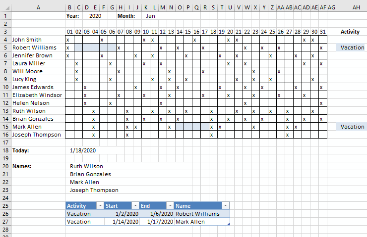
This schedule uses the year and month in cell D1 and K1 to highlight activities like vacation specified in the Excel defined Table. The schedule works like this, enter a date in cell B18 and a formula in cell B20 extracts the names that have an x for the given date.
The names and x are entered manually, however, the activity cells are highlighted automatically based on the start and end date specified in the Excel defined Table.
The date calculations in row 3 are based on the selected year and month, you don't need to change these dates. The activity column AH is based on the name of the activity, start, end date, and the name in the Excel defined Table.
How I built this schedule
Date drop-down list
Cell K1 contains a drop-down list that lets you pick a month, here is how I created it:
- Select cell K1.
- Press with left mouse button on tab "Data" on the ribbon.
- Press with left mouse button on "Data Validation" button.
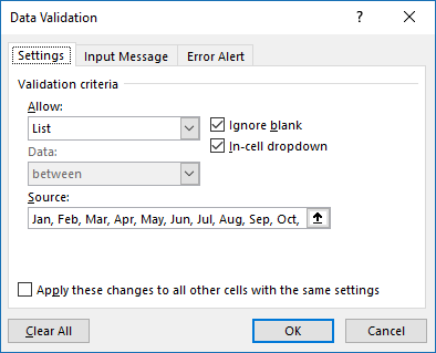
- Choose "List".
- Type "Jan, Feb, Mar, Apr, May, Jun, Jul, Aug, Sep, Oct, Nov, Dec" without double quotes in Source:.
- Press with left mouse button on OK button.
Dates in row 3
These dates are dynamic meaning they change depending on what year and month the user have selected.
Formula in cell B3:
Explaining formula in cell B3
We need to create an Excel date and to do that we have the DATE function. It needs three values, year, month, and day. The month value is a number between 1 and 12. 1 is January is 1, February is 2 and March is 3, etc.
Step 1 - Convert month name to the numerical equivalent
MATCH(K1, {"Jan", "Feb", "Mar", "Apr", "May", "Jun", "Jul", "Aug", "Sep", "Oct", "Nov", "Dec"}, 0)
becomes
MATCH("Jan", {"Jan", "Feb", "Mar", "Apr", "May", "Jun", "Jul", "Aug", "Sep", "Oct", "Nov", "Dec"}, 0)
and returns 1. This means that "Jan" has position 1 in the array. "Jan" is also the first month in a year.
Step 2 - Create Excel date
DATE(D1, MATCH(K1, {"Jan", "Feb", "Mar", "Apr", "May", "Jun", "Jul", "Aug", "Sep", "Oct", "Nov", "Dec"}, 0), 1)
becomes
DATE(D1, 1, 1)
becomes
DATE(2020, 1, 1)
and returns 43831. Excel formats the number as an Excel date and shows only 01 in cell B3.
Formula in cell C3:
This formula is copied to cell range D3:AF3.
Select cell range B3:AH3. Press CTRL + 1 to format cells.
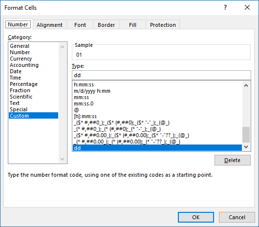
Press with left mouse button on "Custom" and then use type dd to only show the day number. Press with left mouse button on OK button to apply changes.
Conditional formatting
I use conditional formatting to highlight specific date ranges based on the Excel defined Table.
- Select cell range B4:AF16.
- Go to tab "Home" on the ribbon.
- Press with left mouse button on "Conditional Formatting" button.
- Press with left mouse button on "New Rule...".
- Press with left mouse button on "Use a formula to determine which cells to format".
- Type the following formula:
=COUNTIFS(INDIRECT("Table1[Start]"), "<="&B$3,INDIRECT("Table1[End]"), ">="&B$3, INDIRECT("Table1[Name]"), $A4)
- Press with left mouse button on "Format..." button.
- Go to tab "Fill".
- Pick a color.
- Press with left mouse button on OK button.
- Press with left mouse button on OK button.
Explaining Conditional formatting formula in cell B4
The COUNTIFS function counts the number of rows in the Excel defined Table that meets three conditions. Date =< Start, Date =>End, and if name equal to a name in the table. If all three are met then the formula returns 1 and the cell is highlighted.
COUNTIFS(criteria_range1, criteria1, [criteria_range2, criteria2], [criteria_range3, criteria3]…)
The formula also contains cell references that change when the CF moves to the next cell, you can read more about it here: How to use absolute and relative references
Step 1 - Is date in cell B3 larger than or equal to start dates?
criteria_range1 is a cell reference or structured reference to Table1 and column Start. Excel is not happy with structured references in Conditional formatting formulas, however, there is a workaround. Simply use the INDIRECT function and Excel is happy again.
INDIRECT("Table1[Start]")
criteria1 is a cell reference to the date in cell B3. The <= is logical operators that make the COUNTIFS function check that the date in B3 is larger or equal to the dates in Table1[Start]. The ampersand character & concatenates the logical operators and the date in cell B3. The double quotes are needed in order to treat the logical operators as text.
"<="&B$3
Note, the cell references changes to the next cell C$3 when the CF formula moves.
INDIRECT("Table1[Start]"), "<="&B$3
returns
{43832;43844}, "<=43831"
Step 2 - Is date in cell B3 smaller than or equal to end dates?
Here is criteria_range2 and criteria2.
INDIRECT("Table1[End]"), ">="&B$3
returns
{43836;43847}, ">=43831"
Step 3 - Is name in cell $A4 equal to name in Table1?
INDIRECT("Table1[Name]"), $A4
returns
{"Robert Williams";"Mark Allen"}, "John Smith"
Step 4 - All conditions together
COUNTIFS(INDIRECT("Table1[Start]"), "<="&B$3,INDIRECT("Table1[End]"), ">="&B$3, INDIRECT("Table1[Name]"), $A4)
becomes
COUNTIFS({43832;43844}, "<=43831",{43836;43847}, ">=43831", {"Robert Williams";"Mark Allen"}, "John Smith")
and returns 0 (zero). Cell B4 is not highlighted.
Formula in cell AH4
This formula checks if the name and the corresponding start and end dates overlap the selected year and month. It returns the activity name if conditions are met.
Formula in cell B20
You can find an explanation of this formula in the following article: Shift Schedule
Dates category
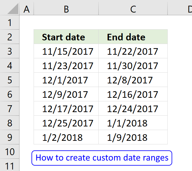
Question: I am trying to create an excel spreadsheet that has a date range. Example: Cell A1 1/4/2009-1/10/2009 Cell B1 […]
This article demonstrates how to return the latest date based on a condition using formulas or a Pivot Table. The […]
This article explains how to search for a specific date and identify a date range in which it falls between […]
Schedule category
Two dimensional lookup category
Table of Contents How to perform a two-dimensional lookup Reverse two-way lookups in a cross reference table [Excel 2016] Reverse […]
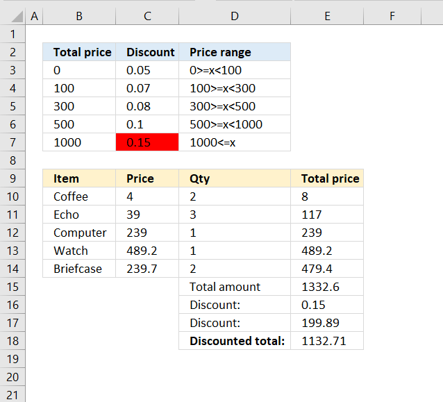
Have you ever tried to build a formula to calculate discounts based on price? The VLOOKUP function is much easier […]
Excel categories
31 Responses to “Get date ranges from a schedule”
Leave a Reply
How to comment
How to add a formula to your comment
<code>Insert your formula here.</code>
Convert less than and larger than signs
Use html character entities instead of less than and larger than signs.
< becomes < and > becomes >
How to add VBA code to your comment
[vb 1="vbnet" language=","]
Put your VBA code here.
[/vb]
How to add a picture to your comment:
Upload picture to postimage.org or imgur
Paste image link to your comment.
Oscar,This is great work...thanks for your time
Oscar you are genius! Thank you!
Geoff,
I am happy you like it!
This was tremendously helpful to me, but is there a way to then reference what other days in the month the resulting names are also scheduled?
Keeping with our example, if Robert, James, and Brian are all scheduled on the 14th, is there a formula to also tell me that at least one of these three will be working on all of the following dates: 1, 3, 4, 7, 8, 9, etc.?
Corrine,
great question!
See attached file:
Shift-scheduling-Corrine.xlsx
[...] Shift Schedule [...]
Is there a way to do it in reverse where you look up the name and it gives you the days, without moving the data around? What part of the formula would change?
Zachary
Yes, it is possible.
Array formula in cell N19:
Copy cell N19 and paste to cells below.
Alright I see, I started to figure it out with switching it out to column instead of row. Although why have the $A$1:A1 at the end? I have it set to go A1, B1, etc. I do have a bit more complicated setup though as it is searching for a mark in a certain cell first then a different mark. So you have x's where I have C's and then T's and then M's. Issue I have is that with the Small formula it tells which number to look for so it doesn't repeat already said numbers but when it gets to the second letter it errors because it is already on the 6th number and not the first where there may not be a 6th number based on the value. Here is my Formula-
{=IFERROR(INDEX('Equipment & Bucket Fitment'!$A$2:$A$2000,SMALL(IF(INDEX('Equipment & Bucket Fitment'!$B$2:$LZ$2000,0,MATCH($A$3,'Equipment & Bucket Fitment'!$B$1:$LZ$1,0))="C",MATCH(ROW('Equipment & Bucket Fitment'!$A$2:$A$2000),ROW('Equipment & Bucket Fitment'!$A$2:$A$2000)),""),ROW('Equipment & Bucket Fitment'!A1))),IFERROR(CONCATENATE(INDEX('Equipment & Bucket Fitment'!$A$2:$A$2000,SMALL(IF(INDEX('Equipment & Bucket Fitment'!$B$2:$LZ$2000,0,MATCH($A$3,'Equipment & Bucket Fitment'!$B$1:$LZ$1,0))="T",MATCH(ROW('Equipment & Bucket Fitment'!$A$2:$A$2000),ROW('Equipment & Bucket Fitment'!$A$2:$A$2000)),""),ROW('Equipment & Bucket Fitment'!A1))),"T"),CONCATENATE(INDEX('Equipment & Bucket Fitment'!$A$2:$A$2000,SMALL(IF(INDEX('Equipment & Bucket Fitment'!$B$2:$LZ$2000,0,MATCH($A$3,'Equipment & Bucket Fitment'!$B$1:$LZ$1,0))="M",MATCH(ROW('Equipment & Bucket Fitment'!$A$2:$A$2000),ROW('Equipment & Bucket Fitment'!$A$2:$A$2000)),""),ROW('Equipment & Bucket Fitment'!A1))),"M")))}
Basically once it finds all the C's it then goes to find all the T's but errors because it is already on the 6th number because of the Small formula. Most times there isn't a 6th T let alone a 3rd, problem is I can't just choose a cell to change back to 1 because the cell varies based on the data referenced.
Zachary,
Although why have the ROWS($A$1:A1) at the end?
It won't break the formula if you insert columns or rows.
Issue I have is that with the Small formula it tells which number to look for so it doesn't repeat already said numbers but when it gets to the second letter it errors because it is already on the 6th number and not the first where there may not be a 6th number based on the value. Here is my Formula
It looks like you can simplify your formula to a great extent. Try using an IF function and use all your criteria in the first argument.
Isn't that what I am doing with IFERROR though? Not sure how I can simplify it. But the problem still stands with it erroring out when searching for the next letter. Even if I implemented an IF and simplified it, how would I get it to reset to 1 when its finished finding all the C's and start at 1 with T's?
Zachary
Even if I implemented an IF and simplified it, how would I get it to reset to 1 when its finished finding all the C's and start at 1 with T's?
If you could look for all C T and M in one logical expression would make it easier but I don't understand your formula.
This part seems to fetch values from a specific column? Why not look in the entire cell range 'Equipment & Bucket Fitment'!$B$2:$LZ$2000 ?
INDEX('Equipment & Bucket Fitment'!$B$2:$LZ$2000,0,MATCH($A$3,'Equipment & Bucket Fitment'!$B$1:$LZ$1,0))
I would like to look for all at one but can't seem to get it in where excel will accept it. Although I do need it to prioritize C's first, then T's, then M's. As for the part you referenced, the only thing that is specific to one spot is the $A$3, which is the cell we enter a value into. $B$2:$LZ$2000 is where all the C's, T's, and M's are. $B$1:$LZ$1 is a range across the top that has some of the data for lookup. Basically, the formula makes it so we can look up a piece of equipment and it shows the attachments that fit or need testing or need modification, the with a few changes it will also be able to look up an attachment and show which machines it fits on. but the issue comes at hand where when going into the second letter Small is already on 4th or 5th or 6th value. When I mean farther ahead, I mean I have 20 cells with this formula and as it goes down the cells the lookup number for the Small formula is going up.
Chart with Letters
https://postimg.org/image/hvl55g1gt/
Sheet with the Formula in It
https://postimg.org/image/b54nw2ywd/
It didn't post my last comment for some reason. Hmmm. well I will just give a quick explaination of the formula. It is almost just like yours but basically repeated a few times. The reason it is harder to lookup all three at the same time is I need to prioritze C's then T's and then M's. Specifically because the C's are more important. And I am using CONCATENATE for T's and M's and adding a letter at the end of the number so I need it to specify that. The iferror makes it so that if it can't find anymore C's then it moves to the formula that looks for T's and once it can't find anymore T's it moves to M's. It uses iferror to separate C's from the T's and M's and then a second iferror within that one to separate T's and M's. The point of the formula is for us to look up machines by their number and have it show the attachments that fit it.
Zachary
Thank you for describing your worksheet in great detail.
Do you really need to have all C M and T in one search formula?
See this example workbook: Zachary.xlsx
We thought about having them separate and if I split the current one up it works like that but we are really trying not to do that.
Zachary,
I understand. The formula in column V in the attached workbook below filters C's first and then M and T's in any order.
Zacharyv2.xlsx
I think I am getting closer.
So at this point I have three working formulas, one of which is mine and two of yours. One of mine and one of yours require the lookup of C, T, and M to be like this {"C","T","M"} and within those array brackets. It works one way but when I reverse it to be able to lookup the opposite value, it does not work when there are multiple letters within those array brackets and I do not know why. The last one is yours and it was the last one you sent me within the Zachary2 document. That one works great and actually works really good with the CONCATENATE formula for T and M, but the only issue is when I have it in 50 cells it runs my computer out of ram. I am running a powerful computer and still run low on ram and cpu trying to process it, it also takes about 10 seconds to process. Otherwise it is the best working one so far.
I did just notice that for some reason, here at work we have 32bit office installed. Maybe swapping to 64bit may help with the processing of the formula.
Zachary
I am happy my formula works great.
the only issue is when I have it in 50 cells it runs my computer out of ram. I am running a powerful computer and still run low on ram and cpu trying to process it, it also takes about 10 seconds to process.
Are there other cpu-intensive formulas in your workbook? Perhaps volatile functions? (Functions that recalculate every time you press F9, like TODAY(), INDIRECT())
https://www.decisionmodels.com/calcsecretsi.htm
There are other formulas that you can tell take a millisecond longer than others as well as they are a lot longer. But the thing is I can run 50 of them without issue and it only starts to become an issue when the one you gave me runs more than 5 of them. I don't use either of those formulas. I did once but not anymore. I use a lot of INDEX, IF, IFERROR, CONCATENATE, VLOOKUP, and MATCH. Even when I removed all other formulas and used just yours it worked up until past 10 of them which then it had to process.
Zachary
Even when I removed all other formulas and used just yours it worked up until past 10 of them which then it had to process.
I see, my array formula is the cause of the problem. I don't know how to make it faster unless a user defined function is an option.
At this point you have helped a great amount with getting the formula I need. At this point it should be tweaking a few things to either make yours process faster or use one the others and make them work correctly. I appreciate all the help you have given and will definitely recommend you to anyone needing help with excel that I can't help with. Thank you Oscar.
Zachary
You are welcome. Thank you for commenting.
I have facing another issues which smart search option,
DB Sheet has three columns which are code,evident,sub-evident
Actual excel sheet I am having 3 column like drop-down menu which based on selection,
for example if I select evident based on evident, code and sub-evident should display, any way should be possible which I want in excel? If you need any question i am feel free to answer for this/
I have a list of parts that has x amount of minutes to produce. I have a limited capacity each week. I would like to create an easy way to create a "matrix" that shows how the production minutes can be distributed from Week to Week. I need to be able to change the capacity as necessary.
Part Total Minutes WK1 WK2 WK3 WK4 WK5
1 280 280
2 2079 1640 439
3 4200 1481 1920 799
4 2552 1121 1431
5 396 396
6 7134 93
7 1476
8 2288
Capacity 1920 1920 1920 1920 1920
Robert Ballard
Is my table correct?
Why is part 2 wk 1 1640 when capacity is 1920?
Hi
Awesome formulas and examples! Have worked a treat for our rota.
One query though - we have a switch-over at 8am on any given day, is there a way to replace "=TODAY()" With "=NOW()" at all? Basically, we're trying to show that before 8am it pulls the individual from the day before TODAY, but at 08:01 it changes to the person with the x in on that day? (Does that make sense?)
Chris,
Yes, it makes sense. Try this:
=IF((NOW() - INT(NOW())) < (8/24), TODAY()-1,TODAY())
Mr Oscar this lesson helped me to complete one of my attendance sheet that I created using excel.I found a way to identify a daily attendance employees names using your formula.but still I have a problem because under my attendance sheet I have 5 types (leave) so I need to find out how can I apply those five leave types for your formula.
this will be big support to complete my attendance sheet sir
so could you explain how to apply different leave types for this same formula that you used about lesson.