How to use the COMBIN function
The COMBIN function returns the number of combinations for a specific number of elements out of a larger number of elements.
Table of Contents
1. Syntax
COMBIN(number, number_chosen)
| number | Required. A whole number larger than 0 (zero) represents the total number of elements. |
| number_chosen | Required. A whole number larger than 0 (zero) represents the number of elements in each combination. |
I recommend you press with left mouse button on the following link if you want to read about the difference between combinations and permutations in greater detail.
2. Example
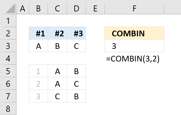
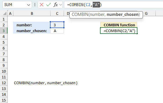
You have 3 different types of fruits and want to make a fruit salad with 2 fruits. If you can't use the same fruit more than once (no repetition), how many different combinations are possible?
Here are the arguments:
- number: 3
- number_chosen: 2
Formula in cell F3:
The formula in cell F3 returns 3 combinations. Column B, C and D demonstrate how many combinations there are when 2 elements are selected out of 3 elements [A, B, C].
The three combinations are [A,B] ,[A,C] and [B,C]. The elements' internal order is not important, that is why [A,B] and [B,A] is the same combination.
The math formula behind the COMBIN function is:
C(n,r) = n!/(r!(n-r)!)
C = Combinations
n = objects (number)
r = sample (number_chosen)
Lets use the values given in the question and manually calculate the value.
3!/(2!(3-2)!)
=3*2/2*1
=6/2
=3
The math formula calculates number 3 which represents the number of combinations with 3 objects and 2 chosen. This value matches the calculated value in cell F3.
3. COMBIN Function alternative

Here is how the COMBIN function calculates in greater detail, see the image above. The formula below is the same as the formula shown in the image above, FACT function is the ! (factorial character).
The text representation is:
C(n,r) = n!/(r!(n-r)!)
C = Combinations
n = objects (number)
r = sample (number_chosen)
Formula in cell C7:
3.1 Explaining formula
Step 1 - Calculate the numerator
The FACT function calculates the factorial of a number.
FACT(number)
FACT(C5)
becomes
FACT(3)
and returns 6. 3*2*1 equals 6.
Step 2 - Calculate the denominator
(FACT(C6)*FACT(C5-C6))
C5-C6
becomes
3-2 and returns 1.
FACT(1) is 1.
FACT(2) is 2. 2*1 equals 2.
The parentheses let you control the order of operation.
(FACT(C6)*FACT(C5-C6))
becomes
2*1 equals 2.
Step 3 - Calculate the division
FACT(C5)/(FACT(C6)*FACT(C5-C6))
becomes
6/2 equals 3.
4. List combinations - Excel 365 formula

This section demonstrates how to list all combinations based on n (numbers) and r (numbers_chosen). The following formula works only in Excel 365 and it spills values to the right and to cells below as far as needed.
Check out this article: Return all combinations that describes a User Defined Function that lists combinations. That UDF should work for most Excel versions.
Excel 365 dynamic array formula in cell I2:
The formula has three arguments:
- objects: C2:C7 (This populates the list of combinations with the given values, this example uses A to F.
- n: F2 (The total number of objects, this value must match the number of values in argument objects)
- r: F3 (The number chosen)
The image above shows a table in cell range I2:N16 containing all possible combinations with 4 objects chosen from a group of 6 objects in total. The formula populates the table with the specified values in C2:C7 accordingly.
The table is built dynamically meaning if you change the input arguments the table changes it size almost instantly. Make sure you use the same number of values in cell range C2:C7 as the specified number in cell F2.
4.1 Explaining formula
Step 1 - To the power of
This step calculates the number of rows needed to calculate every combination.
2^F2
becomes
2^6 equals 64.
Step 2 - Create an array from 0 (zero) to n
The SEQUENCE function creates a sequence of numbers.
SEQUENCE(rows, [columns], [start], [step])
SEQUENCE(2^F2)-1
becomes
SEQUENCE(64)-1
becomes
{1; 2; 3; ... ; 64} - 1
and returns
{0; 1; 2; 3; ... ; 63}.
Step 3 - Divide vertical array by horizontal array
(SEQUENCE(2^F2)-1)/2^SEQUENCE(,F2,0)
becomes
{0; 1; 2; 3; ... ; 63}/2^SEQUENCE(,F2,0)
becomes
{0; 1; 2; 3; ... ; 63}/2^{0,1,2,3,4,5}
becomes
{0; 1; 2; 3; ... ; 63}/{1,2,4,8,16,32}
and returns
{0, 0, 0, 0, 0, 0;1, ... , 1.96875}.
Step 3 - Remove decimals
The INT function removes the decimal part from positive numbers and returns the whole number (integer) except negative values are rounded down to the nearest integer.
INT(number)
INT((SEQUENCE(2^F2)-1)/2^SEQUENCE(,F2,0))
becomes
INT({0, 0, 0, 0, 0, 0;1, ... , 1.96875})
and returns
{0, 0, 0, 0, 0, 0; 1, ... , 1}
Step 4 - Calculate the remainder
The MOD function returns the remainder after a number is divided by a divisor.
MOD(number, divisor)
MOD(INT((SEQUENCE(2^F2)-1)/2^SEQUENCE(,F2,0)),2)
becomes
MOD({0, 0, 0, 0, 0, 0; 1, ... , 1}, 2)
and returns
{0, 0, 0, 0, 0, 0; 1, ... , 1}.
Step 5 - Calculate the matrix product of two arrays
The MMULT function calculates the matrix product of two arrays, an array as the same number of rows as array1 and columns as array2.
MMULT(array1, array2)
MMULT(MOD(INT((SEQUENCE(2^F2)-1)/2^SEQUENCE(, F2,0)), 2), SEQUENCE(F2)^0)
becomes
MMULT({0, 0, 0, 0, 0, 0; 1, ... , 1}, {1; 1; 1; 1; 1; 1})
and returns
{0; 1; 1; 2; 1; ... ; 6}
Step 6 - Check if number is equal to numbers_chosen
The equal sign lets you compare value to value in an Excel formula, the result is a boolean value TRUE or FALSE.
MMULT(MOD(INT((SEQUENCE(2^F2)-1)/2^SEQUENCE(,F2,0)),2),SEQUENCE(F2)^0)=F3
becomes
{0; 1; 1; 2; 1; ... ; 6}=4
and returns
{FALSE; FALSE; FALSE; FALSE; ... ; FALSE}
Step 7 - Filter combinations based on the number chosen
The FILTER function lets you extract values/rows based on a condition or criteria.
FILTER(array, include, [if_empty])
FILTER(MOD(INT((SEQUENCE(2^F2)-1)/2^SEQUENCE(,F2,0)),2),MMULT(MOD(INT((SEQUENCE(2^F2)-1)/2^SEQUENCE(,F2,0)),2),SEQUENCE(F2)^0)=F3)
becomes
FILTER(MOD(INT((SEQUENCE(2^F2)-1)/2^SEQUENCE(,F2,0)),2),{FALSE; FALSE; FALSE; FALSE; ... ; FALSE})
becomes
FILTER({0, 0, 0, 0, 0, 0; 1, ... , 1},{FALSE; FALSE; FALSE; FALSE; ... ; FALSE})
and returns
{1, 1, 1, 1, 0, 0;
1, 1, 1, 0, 1, 0;
1, 1, 0, 1, 1, 0;
1, 0, 1, 1, 1, 0;
0, 1, 1, 1, 1, 0;
1, 1, 1, 0, 0, 1;
1, 1, 0, 1, 0, 1;
1, 0, 1, 1, 0, 1;
0, 1, 1, 1, 0, 1;
1, 1, 0, 0, 1, 1;
1, 0, 1, 0, 1, 1;
0, 1, 1, 0, 1, 1;
1, 0, 0, 1, 1, 1;
0, 1, 0, 1, 1, 1;
0, 0, 1, 1, 1, 1}
Step 8 - Populate the array
The IF function returns one value if the logical test is TRUE and another value if the logical test is FALSE.
IF(logical_test, [value_if_true], [value_if_false])
IF(FILTER(MOD(INT((SEQUENCE(2^F2)-1)/2^SEQUENCE(,F2,0)),2),MMULT(MOD(INT((SEQUENCE(2^F2)-1)/2^SEQUENCE(,F2,0)),2),SEQUENCE(F2)^0)=F3),TRANSPOSE(C2:C7),"")
becomes
IF({1, 1, 1, 1, 0, 0;
1, 1, 1, 0, 1, 0;
1, 1, 0, 1, 1, 0;
1, 0, 1, 1, 1, 0;
0, 1, 1, 1, 1, 0;
1, 1, 1, 0, 0, 1;
1, 1, 0, 1, 0, 1;
1, 0, 1, 1, 0, 1;
0, 1, 1, 1, 0, 1;
1, 1, 0, 0, 1, 1;
1, 0, 1, 0, 1, 1;
0, 1, 1, 0, 1, 1;
1, 0, 0, 1, 1, 1;
0, 1, 0, 1, 1, 1;
0, 0, 1, 1, 1, 1},TRANSPOSE(C2:C7),"")
The TRANSPOSE function allows you to convert a vertical range to a horizontal range, or vice versa.
TRANSPOSE(array)
TRANSPOSE(C2:C7)
becomes
TRANSPOSE({"A"; "B"; "C"; "D"; "E"; "F"})
and returns
{"A", "B", "C", "D", "E", "F"}.
IF({1, 1, 1, 1, 0, 0;
...
0, 0, 1, 1, 1, 1},TRANSPOSE(C2:C7),"")
becomes
IF({1, 1, 1, 1, 0, 0;
...
0, 0, 1, 1, 1, 1},{"A", "B", "C", "D", "E", "F"},"")
and returns
{"A", "B", "C", "D", "", "";
"A", "B", "C", "", "E", "";
"A", "B", "", "D", "E", "";
"A", "", "C", "D", "E", "";
"", "B", "C", "D", "E", "";
"A", "B", "C", "", "", "F";
"A", "B", "", "D", "", "F";
"A", "", "C", "D", "", "F";
"", "B", "C", "D", "", "F";
"A", "B", "", "", "E", "F";
"A", "", "C", "", "E", "F";
"", "B", "C", "", "E", "F";
"A", "", "", "D", "E", "F";
"", "B", "", "D", "E", "F";
"", "", "C", "D", "E", "F"}
Step 9 - Simplify formula
The LET function lets you name intermediate calculation results which can shorten formulas considerably and improve performance.
LET(name1, name_value1, calculation_or_name2,
[name_value2, calculation_or_name3...])
IF(FILTER(MOD(INT((SEQUENCE(2^F2)-1)/2^SEQUENCE(,F2,0)),2),MMULT(MOD(INT((SEQUENCE(2^F2)-1)/2^SEQUENCE(,F2,0)),2),SEQUENCE(F2)^0)=F3),TRANSPOSE(C2:C7),"")
x - MOD(INT((SEQUENCE(2^y)-1)/2^SEQUENCE(, y, 0)), 2)
y - F2
LET(y, F2, x, MOD(INT((SEQUENCE(2^y)-1)/2^SEQUENCE(, y, 0)), 2), IF(FILTER(x, MMULT(x, SEQUENCE(y)^0)=F3), TRANSPOSE(C2:C7), ""))
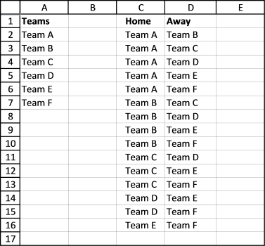
5. Test combinations (Solver)

The Solver is an Excel feature that can test combinations in order to find the best combination based on a condition or criteria. This example shows parcel names in column B, weight in column C, and the value in column D.
Which combination of four parcels out of 11 has the highest value if the total weight is lower than or equal to 291?
Total weight formula in cell F16:
Total value formula in cell F17:
5.1 Explaining the total weight formula
Step 1 - Compare values
The equal sign is a logical operator that lets you check if a value is equal to another value, in this case, multiple values to a single value.
The Excel Solver changes the numbers, 1 or 0 (zero), in cells F3:F13. We use these values to calculate the total weight for each combination.
F3:F13=1
Step 2 - Control the order of operation
The parentheses lets you control the order of intermediate calculations, we want to compare F3:F13 to 1 before we multiply by C3:C13.
(F3:F13=1)
Step 3 - Multiply
The asterisk character lets you multiply values and arrays in an Excel formula.
(F3:F13=1)*C3:C13
Step 4 - Calculate a total
The SUMPRODUCT function calculates the product of corresponding values and then returns the sum of each multiplication.
SUMPRODUCT(array1, [array2], ...)
SUMPRODUCT((F3:F13=1)*C3:C13)
5.2 Setting up the Excel Solver

- Go to the tab "Data" on the ribbon.
- Press the left mouse button on the "Solver" button.
- Press the left mouse button on the arrow next to "Set Objective" and select cell F17. This value is F3:F13 multiplied by D3:D13 and then summarized.
- Press the left mouse button on the radio button named "Max" to select it. This lets the solver know that we are looking for a combination that returns the largest sum.
- Press with left mouse button on the arrow next to "By changing variable cells" and select cells F3:F13. These cells changes between 1 and 0 (zero).
- Press with the left mouse button on the "Add" button. A dialog box appears, this lets you apply constraints. Add the constraints shown in the image above specifiied below "Subject to the Constraints:".
- Change solving method to "Evolutionary".
- Press with the mouse on the check box "Make unconstrained variables Non-negative to enable it.
- Press with left mouse button on the "Solve" button to start.
- A dialog box appears after some time, press the left mouse button on the "OK" button.
Useful links
COMBIN function - Microsoft
COMBIN function
7. Return all combinations
Today I have two functions I would like to demonstrate, they calculate all possible combinations from a cell range. What is a combination? To explain combinations I must explain the difference between combinations and permutations.
Think of permutations as if the order is important and combinations as if the order is not important. If this is confusing, look at the following examples.
Example 1 - Permutations
 Think of a phone number, each digit can be between 0 to 9 or 10 different values. A five digit phone number contains 100 000 permutations (10x10x10x10x10 equals 100 000).
Now imagine a phone number to a friend or co-worker. If we rearrange the phone numbers, you could possibly call a stranger. The order is important.
Read this article to learn more about permutations:
Recommended articles
I discussed the difference between permutations and combinations in my last post, today I want to talk about two kinds […]
Example 2 - Combinations
 Imagine you are about to buy a pizza and you can choose from five ingredients, cheese, tomato sauce, onions, ham, and mushrooms. It doesn´t matter in what order you say the ingredients. The order is not important.
A five-digit phone number has 100 000 possible permutations but five out of five pizza ingredients have only one combination. I guess only mathematicians use the word permutations, everyone else uses the word combinations even if they talk about permutations.
The following article demonstrates a problem solved with combinations, the order is not important:
Recommended articles
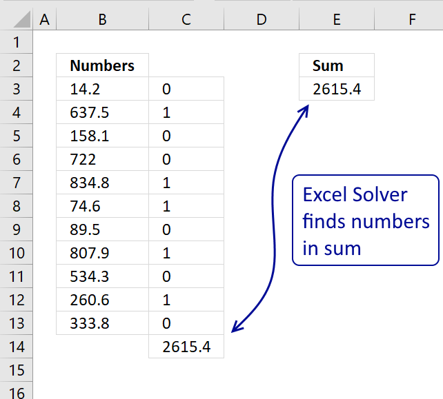
Table of Contents Identify numbers in sum using Excel solver Find numbers in sum - UDF Find positive and […]
User defined functions
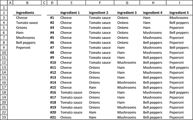
The following User Defined Function lets you, for example, see all the combinations of pizza ingredients you can choose from if you pick 5 out of 7 ingredients.
Update 7/1/2022! There is now an Excel 365 formula that also lists combinations: List combinations - Excel 365 formula
Custom array formula in cell range E3:I23:
You need to copy the VBA code below to your workbook before you try the above User Defined Function.
Watch this video to learn more about the UDF
How to enter an array formula
- Select cell range E3:I23
- Press with left mouse button on in fomula bar
- Enter custom function
- Press and hold CTRL + SHIFT
- Press Enter
If you did it right the formula now begins and ends with curly brackets, like this {=array formula}. They appear automatically, don´t enter the curly brackets yourself.
Recommended articles

Array formulas allows you to do advanced calculations not possible with regular formulas.
VBA Code
'Dimension public variable and declare data type
Public result() As Variant

'Name User Defined Function
Function Combinations(rng As Range, n As Single)

'Save values from cell range rng to array variable rng1
rng1 = rng.Value

'Redimension array variable result
ReDim result(n - 1, 0)

'Start User Defined Function Recursive with paramters rng1, n, 1, 0
Call Recursive(rng1, n, 1, 0)

'Remove a column of values from array variable result
ReDim Preserve result(UBound(result, 1), UBound(result, 2) - 1)¨

'Transpose values in variable result and then return result to User Defined Function on worksheet
Combinations = Application.Transpose(result)

End Function
'Name User Defined Function and paramters
Function Recursive(r As Variant, c As Single, d As Single, e As Single)

'Dimension variables and declare data types
Dim f As Single

'For ... Next statement
For f = d To UBound(r, 1)

'Save value in array variable r row f column 1 to array variable result row e and last column
result(e, UBound(result, 2)) = r(f, 1)

'If ... Then ... Else ... End If statement
'Check if variable in e is equal to c -1
If e = (c - 1) Then

'Add another column to array variable result
ReDim Preserve result(UBound(result, 1), UBound(result, 2) + 1)

'For ... Next statement
For g = 0 To UBound(result, 1)

'Save value in array variable result row g second last column to result row g last column
result(g, UBound(result, 2)) = result(g, UBound(result, 2) - 1)
Next g

'Continue here if e is not equal to c - 1
Else

'Start User Defined Function Recursive with parameters r, c, f + 1, e + 1
Call Recursive(r, c, f + 1, e + 1)
End If

Next f

End Function
These functions have a limit of 65532 rows, if you need more read this comment.
Where to copy vba code?
- Go to VB Editor (Alt + F11)
- Press with left mouse button on "Insert" on the menu
- Press with left mouse button on "Module"
- Paste code to code module
- Return to excel
Tip! Did you know that Excel can calculate the number of combinations for you? Use the COMBIN function:
=COMBIN(7,5) equals 21 combinations.
8. Function not working
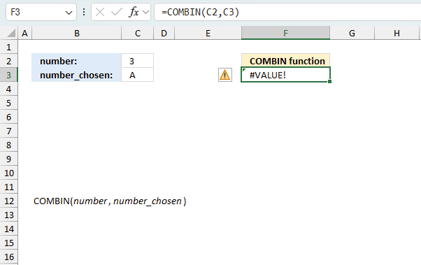
The COMBIN function returns
- #VALUE! error if any of the arguments is a non-numeric value.
- #NAME? error if you misspell the function name.
- propagates errors, meaning that if the input contains an error (e.g., #VALUE!, #REF!), the function will return the same error.
8.1 Troubleshooting the error value
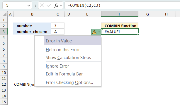
When you encounter an error value in a cell a warning symbol appears, displayed in the image above. Press with mouse on it to see a pop-up menu that lets you get more information about the error.
- The first line describes the error if you press with left mouse button on it.
- The second line opens a pane that explains the error in greater detail.
- The third line takes you to the "Evaluate Formula" tool, a dialog box appears allowing you to examine the formula in greater detail.
- This line lets you ignore the error value meaning the warning icon disappears, however, the error is still in the cell.
- The fifth line lets you edit the formula in the Formula bar.
- The sixth line opens the Excel settings so you can adjust the Error Checking Options.
Here are a few of the most common Excel errors you may encounter.
#NULL error - This error occurs most often if you by mistake use a space character in a formula where it shouldn't be. Excel interprets a space character as an intersection operator. If the ranges don't intersect an #NULL error is returned. The #NULL! error occurs when a formula attempts to calculate the intersection of two ranges that do not actually intersect. This can happen when the wrong range operator is used in the formula, or when the intersection operator (represented by a space character) is used between two ranges that do not overlap. To fix this error double check that the ranges referenced in the formula that use the intersection operator actually have cells in common.
#SPILL error - The #SPILL! error occurs only in version Excel 365 and is caused by a dynamic array being to large, meaning there are cells below and/or to the right that are not empty. This prevents the dynamic array formula expanding into new empty cells.
#DIV/0 error - This error happens if you try to divide a number by 0 (zero) or a value that equates to zero which is not possible mathematically.
#VALUE error - The #VALUE error occurs when a formula has a value that is of the wrong data type. Such as text where a number is expected or when dates are evaluated as text.
#REF error - The #REF error happens when a cell reference is invalid. This can happen if a cell is deleted that is referenced by a formula.
#NAME error - The #NAME error happens if you misspelled a function or a named range.
#NUM error - The #NUM error shows up when you try to use invalid numeric values in formulas, like square root of a negative number.
#N/A error - The #N/A error happens when a value is not available for a formula or found in a given cell range, for example in the VLOOKUP or MATCH functions.
#GETTING_DATA error - The #GETTING_DATA error shows while external sources are loading, this can indicate a delay in fetching the data or that the external source is unavailable right now.
8.2 The formula returns an unexpected value
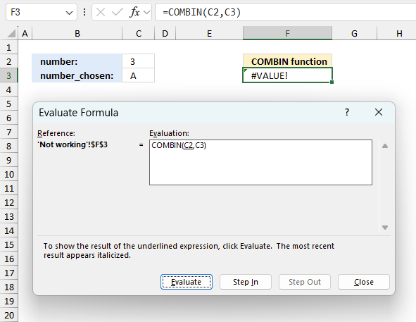
To understand why a formula returns an unexpected value we need to examine the calculations steps in detail. Luckily, Excel has a tool that is really handy in these situations. Here is how to troubleshoot a formula:
- Select the cell containing the formula you want to examine in detail.
- Go to tab “Formulas” on the ribbon.
- Press with left mouse button on "Evaluate Formula" button. A dialog box appears.
The formula appears in a white field inside the dialog box. Underlined expressions are calculations being processed in the next step. The italicized expression is the most recent result. The buttons at the bottom of the dialog box allows you to evaluate the formula in smaller calculations which you control. - Press with left mouse button on the "Evaluate" button located at the bottom of the dialog box to process the underlined expression.
- Repeat pressing the "Evaluate" button until you have seen all calculations step by step. This allows you to examine the formula in greater detail and hopefully find the culprit.
- Press "Close" button to dismiss the dialog box.
There is also another way to debug formulas using the function key F9. F9 is especially useful if you have a feeling that a specific part of the formula is the issue, this makes it faster than the "Evaluate Formula" tool since you don't need to go through all calculations to find the issue.
- Enter Edit mode: Double-press with left mouse button on the cell or press F2 to enter Edit mode for the formula.
- Select part of the formula: Highlight the specific part of the formula you want to evaluate. You can select and evaluate any part of the formula that could work as a standalone formula.
- Press F9: This will calculate and display the result of just that selected portion.
- Evaluate step-by-step: You can select and evaluate different parts of the formula to see intermediate results.
- Check for errors: This allows you to pinpoint which part of a complex formula may be causing an error.
The image above shows cell reference C3 converted to hard-coded value using the F9 key. The COMBIN function requires numerical values which is not the case in this example. We have found what is wrong with the formula.
Tips!
- View actual values: Selecting a cell reference and pressing F9 will show the actual values in those cells.
- Exit safely: Press Esc to exit Edit mode without changing the formula. Don't press Enter, as that would replace the formula part with the calculated value.
- Full recalculation: Pressing F9 outside of Edit mode will recalculate all formulas in the workbook.
Remember to be careful not to accidentally overwrite parts of your formula when using F9. Always exit with Esc rather than Enter to preserve the original formula. However, if you make a mistake overwriting the formula it is not the end of the world. You can “undo” the action by pressing keyboard shortcut keys CTRL + z or pressing the “Undo” button
8.3 Other errors
Floating-point arithmetic may give inaccurate results in Excel - Article
Floating-point errors are usually very small, often beyond the 15th decimal place, and in most cases don't affect calculations significantly.
'COMBIN' function examples
This article demonstrates macros that create different types of round-robin tournaments. Table of contents Basic schedule - each team plays […]
'COMBIN' function examples
Table of Contents Identify numbers in sum using Excel solver Find numbers in sum - UDF Find positive and […]
This article demonstrates solver in Excel. Table of Contents Introduction Optimize machine efficiency Using Excel Solver to schedule employees Cash […]
This article demonstrates how to solve simultaneous linear equations using formulas and Solver. The variables have the same value in […]
Functions in 'Math and trigonometry' category
The COMBIN function function is one of 62 functions in the 'Math and trigonometry' category.
Excel function categories
Excel categories
64 Responses to “How to use the COMBIN function”
Leave a Reply
How to comment
How to add a formula to your comment
<code>Insert your formula here.</code>
Convert less than and larger than signs
Use html character entities instead of less than and larger than signs.
< becomes < and > becomes >
How to add VBA code to your comment
[vb 1="vbnet" language=","]
Put your VBA code here.
[/vb]
How to add a picture to your comment:
Upload picture to postimage.org or imgur
Paste image link to your comment.
I am working on a udf version without Redim Preserve.
Public result() As Variant

Function Combinations(rng As Range, n As Single)
Dim b As Single

rng1 = rng.Value
b = WorksheetFunction.Combin(UBound(rng1, 1), n)

ReDim result(b, n - 1)
Call Recursive(rng1, n, 1, 0, 0)

For g = 0 To UBound(result, 2)
     result(UBound(result, 1), g) = ""
Next g

Combinations = result

End Function
Function Recursive(r As Variant, c As Single, d As Single, e As Single, h As Single) Dim f As Single For f = d To UBound(r, 1) result(h, e) = r(f, 1) If e = (c - 1) Then For g = 0 To UBound(result, 2) result(h + 1, g) = result(h, g) Next g h = h + 1 Else Call Recursive(r, c, f + 1, e + 1, h) End If Next f End FunctionHi Oscar,
Could we extend this formula to the next page and so on so that the combinations continues to be generated from where it left off in the previous page, because the results stops being generated at row 1048576 (last row in excel). It would be a great help, thanks.
Works great; however, I wonder if a modification can be made such
that each item in the list can be used multiple times; e.g for a
list of 1 2 3 4 "=COMBINATIONS(A1:A4,3)" can yield:
111 112 113 114 etc as well
instead of only: 123 124 134 234
Note: Sequence is not significant so 112, 211 and 121 should be considered the same and therefore shown only once.
Further to my request of April 17, I have looked at the ListPermut Function provided at https://www.get-digital-help.com/excel-udf-list-permutations-with-repetition/.
Although this Function does allow repetitions, it only accepts a single parameter and does not allow specifying the number of terms that form a set. For example, my list contains 8b items while I need to display all permutations/combinations with, say, only 3 out of 8 items at a time.
Found what I am looking for at:
https://www.get-digital-help.com/select-numbers-in-each-permutation/
Thanks.
Thank you so much this is almost what I need, it only allows cheese to appear in gradient #1 I would like see all variation
Cheese as ingredient 1, cheese as ingredient #2, cheese as ingredient 3 ect ect.
[…] Copy the following code to a module. How to insert a module to a workbook. […]
Hi! Thanks, this is very helpful! However, I tried running this for combinations of 24 choices, with 5 picks [basically, =combin(24,5), and it worked fine. When I tried it for 26 choices, with 5 picks, it doesn't work anymore. I tried it with 25 choices and it works... so I assume it's a limitation issue? Appreciate your help. :)
I have a number say 9347. I need all the 4 digit combinations of the number. ie 24 combinations . Is there any VB program in excel to display all the 24 combinations?
9347
9437
9374...etc
Thanks
Krish
[…] can read about the difference between combinations and permutations here: Return all combinations but in short, the order is important for permutations and not important for […]
How would I add more things to choose from Im trying to do 10 things to select.
john,
Add more ingredients to column B.
Change the custom function to:
=Combinations(B3:B12,5) + CTRL + SHIFT + ENTER
B3:B12 contains 10 things.
Hello, Thanks for sharing.. .. Its almost what I was looking for..but my assignment is slightly tricky..
Only additional query for above is.. Above code generates combination with repetitions ... What if we need to have say set of 10 men & need to form 3 member teams and carryout 9 distinct tasks.(Each man should do all 9 tasks). However no two men should repeat working with another man in another task after working with him once in a task. That's 10 men working in 3member teams working only once with rest of 9 members on the 9 tasks.
Your above code should work fine, if repetition of pairs is handled... Is this is even possible? Thanks
HI, I am trying to use this combinations functions on a bigger database. I have 96 items and I want to combine 3 at a time. So the combinations would lead to 96C3 = 142880. Can you please tell me help me with this?
Thanks,
Ajit
Ajit
The following macro lets you build all combinations:
Sub ListPermut()
Dim ws As Worksheet, Ans As String, ans1() As String, digits As Integer
Dim num As Integer, p As Long, i As Long, t As Long
Dim rng() As Long, c As Long, rng1() As String

Set ws = Sheets.Add

Ans = InputBox("How many items?")
digits = InputBox("How many combined?")

For i = 1 To Ans
    tmp = tmp & i & ","
Next i

ans1 = Split(Left(tmp, Len(tmp) - 1), ",")
num = UBound(ans1) + 1

p = Application.WorksheetFunction.Combin(num, digits)


ReDim rng(1 To digits)
ReDim rng1(1 To digits)

For c = 1 To digits
  rng(c) = c
Next c

i = 0
Application.ScreenUpdating = False

Do Until (i + t) = (p - 1)

    For c = LBound(rng1) To UBound(rng1)
        rng1(c) = ans1(rng(c) - 1)
    Next c

    ws.Range("A1").Resize(, digits).Offset(i) = rng1

    rng(digits) = rng(digits) + 1

    If rng(digits) > num Then
        For c = digits - 1 To 1 Step -1
            If rng(c) <> num + c - digits Then
                rng(c) = rng(c) + 1
                Exit For
            End If
        Next c

        For d = c + 1 To digits
            rng(d) = rng(d - 1) + 1
        Next d
    End If

    i = i + 1

    If i = 1000000 Then
        Set ws = Sheets.Add
        t = t + 1000000
        i = 0
    End If

Loop
For c = LBound(rng1) To UBound(rng1)
    rng1(c) = ans1(rng(c) - 1)
Next c
ws.Range("A1").Resize(, digits).Offset(i) = rng1
Application.ScreenUpdating = True

End Sub
Type 96 in the first inputbox and 3 in the second.
Macro inserts a new sheet and returns all combinations (rep not allowed).
Get the Excel *.xlsm file
ListCombinationsv2.xlsm
Hi oscar.
I need an excel macro that print all posible combinations. I have an array from 1 to 42. An i want to pick 6 numbers with no repetitions. Can you help?
Thanks
Hello Ajit, were you successful on the use of the sugessted macro for your 96c3?
I am in awe of this macro, Oscar. Thank you very much. It worked like a charm. Many thanks,
Joey
Joey Godalla
Thank you for your comment.
Fantastic, I finally think I'm in the right place...
Yes I need to see the combinations however, my problem has a constraint.
For example there are 50 balls and 10 baskets, each basket can hold a maximum of 7 balls. What are the possible combinations and how can I list them.
Can the vba be linked to a cell that be can changed to to alter the number of balls, baskets, and maximum capacity per basket.
All the best, Oliver
Hi Oscar & all,
This looks perfect for what I am after; however, I am getting an error message when doing the array formula, saying
'Ambiguous name detected: Combinations'
and then a #NAME? error in all output cells (E3:I23).
I have tried re-pasting the VBA etc and no luck - any tips / ideas?
Many thanks in advance,
Kristina
Kristina,
'Ambiguous name detected: Combinations'
You have two macros with the same name.
...Trying out the macro written for Ajit on 5/12/16.
This one works great returning combinations of numbers up to the input value - is there any way to amend to return combinations of a certain input range (e.g. CHeese, Ham etc etc) as per the original macro?
THanks again!
Kristina,
Use INDEX function to fetch values from an input range.
Great, thank you! This appears to work now :)
Much appreciated!
How exactly do you use INDEX in this case?
Hi, how can we use index i ths case to get the original data like cheese, ham etc.
Thanks
Hello,
How can I get excel to determine all combinations for a specific number within a 12(rows) x 4(columns) table. The tricky part is I am only interested in the combinations for numbers connecting to the selected value. See example blow;
If my specific value is 1(third row)then I would be interested in listing all 4 digit combinations starting with a number connected to it in all directions.
(down) (up)
1,5,9,3 1,7,3,2
1,5,9,2 1,7,3,4
1,5,9,4 1,7,8,4
1,5,9,8 1,7,6,2
1,5,9,0 1,7,2,1
1,5,6,0 1,7,6,0
1,5,6,2
1,5,4,3
1,5,4,7
12 x 4 table
1234
5678
9012
3456
7890
1234
5678
9012
3456
7890
1234
5678
Hi Oscar,
Your Macro is great. I am creating a large number of combination. 90 items, 9 combined. Understandably, it takes a loooong time and often runs out of memory. Is there a way for me to alter your Macro so that i can do it in pieces?
In other words, can i alter it so that instead of the array starting at
1 2 3 4 5 6 7 8 9
1 2 3 4 5 6 7 8 10
that it starts at the 2s, like
2 3 4 5 6 7 8 9 10 ?
Thank you very much
Hi oscar,
Also in addition to starting it from the 2's like i mention above (previous email), can i also alter the macro to STOP generating after it is done with the 2's?
hope that makes sense.
Thanks :)
Thanks so much Oscar! This was exactly what I needed.
Travis,
Thank you for commenting.
Hi Oscar, thanks a lot for the codes.
I have a problem with the volume of data I'm dealing with, it's a combination of 5 out of 160 data points, making around 800 million groups(800 sheets)!
I tested your code for a combination of 5 out of 100, and excel showed up with an error saying there is not enough resources!
What can I do to capture all the combinations?!
thanks.
Keivan,
You could save each sheet as a workbook as they are created, however you would end up with 800 workbooks.
Would that work?
Thank you for this code! Can your function be adapted to to see all possible combinations of 7 items (ingredients), not just combinations of 5 of the 7, for example. (And I do want combinations, not permutations.)
Thank you for any suggestions!
Sally
Use the COMBIN function in excel to see how many combinations you get with 7 values out of 7 values.
=COMBIN(7,7) returns 1.
I think you are looking for permutations?
Excel udf: List permutations without repetition
Excel udf: List permutations with repetition
Thanks for great function. How can I list the combination into row only. Example combinations(A1:A5,2) will generate result into row 1, 2, 3, 4 (1 column only)
Appreciate your job.
Hi Oscar,
Good day.
How can i continue the list after #21, as i have total of 84 combinations.
Thank you
Hello Oscar,
can you please help me out with the following part of my VBA code:
.....
Set BranchXX = Range(Cells(3, 2), Cells(fin, 3))
Set BranchKK = Range(Cells(3, 1), Cells(nr_row, 1))
BranchXX.Select
Selection.FormulaArray = "=Combinations(BranchKK,2)"
I use your function: Combinations and the above code gives an error.
Although if I change the inputs of the function like below everything works fine:
...
Set BranchXX = Range(Cells(3, 2), Cells(fin, 3))
'Set BranchKK = Range(Cells(3, 1), Cells(nr_row, 1))
BranchXX.Select
Selection.FormulaArray = "=Combinations(RC[-1]:R[5]C[-1],2)"
Although I want the first argument of the function to be variable(depending on nr_row ) and need to implement the code like the way I did it firstly
Thank you very much!!
Please provide me with your email address to send you my request
Hi Oscar, I need help with trying to create a number generator that has specific filters for 5-45 numbers with no repeats!!
Is there a you tube step-by-step instruction tutorial on how a beginner can go about creating a number generator for a lottery matrix of 5/45, 5/69,5/70 and 6/39 and so forth ?
hi oscar
i need macros code for 22 alphabets (array) in 11 combination in excel
Sir,
When I Set Range (22,11) in Combinations UDF it show #VALUE. how can i solve.
KP,
try the macro I posted on the December 5, 2016 at 1:59 pm. The Combinations UDF has a limit of 65532 rows.
Hi, I have gone through a lot of such posts. But could not find the dumbest VBA combination algo so far. What I need is this, the combination generator for N (4) picked items with K (2) types (obvious repeat)
the total combination set becomes N+1 = 5
AAAA
AAAB
AABB
ABBB
BBBB
Thanks in advance.
123
124
125
234
235
345
how we build it in query access
not sql
but query eccess
Hİ
!!!!
I am writing to you from Turkey. I'm a student and I have an urgent homework. I have 290 rows of data in my hand.
This combination of 290 data needs to derive 2,3,4,5,6,7,8 combinations.Sample data:
1. a01b
2. a02B
3. a03c
4.
..
290.x02w
data such as.
my excel knowledge is weak. If you have a macro formula, please write to me. can you please help me?
for excample:
a01b-a01c : Combination of 2
...
a01b-a01c-a01d-a01h-a01f : combination of 5
...
a01h-a01f-a01b-a01c- a02c-a03a-a02s-a012 : combination of 8;
That's the way I need it.
Please
Please
waiting for help
[…] shown here in cells A3 through G5042. This file already has what you need, but here is how you can create your own set of combinations for different numbers of […]
following on from Arits VBA code,
How would you add a rule that the combinations cant be more than 4 consecutive numbers in the generated sequence?
Permutation and Group Speed Dating Scenario.
I'm looking to use a modified permutation to create a seating list.
Input is the number tables 5, number seats 5 and list of members 10.
Input
Member 1
Member 2
Member 3
Member 4
Member 5
Member 6
Member 7
Member 8
Member 9
Member 10
Needed Output where the numbers in the round columns are the table assigments for each member as we rearrange members every 15 minutes. Every members should only meet every other member 1 time.
Members Round 1 Round 2 Round
Member 1 1 2 3
Member 2
Member 3
Member 4
Member 5
Member 6
Member 7
Member 8
Member 9
ALL COMBINATIONS
IS WORKING NICE HOWEVER WHEN I TYPE 26 AND 5 WERE YOU COMMENT TO ONE OF THE USERS IS GIVING ME ALL THE COMBINATIONS FROM 1 TO 26 BUT I NEED FOR CERTAIN NUMBERS AND HOW MUCH I TRIED I JUST COULD'NT MODIFY THE CODE TO FIT MY PURPOSE
PLEASE IF YOU CAN GIVE ME AN IDEA ON HOW TO ADD THE RIGHT SHEET AND THE RIGHT RANGE FOR MY NUMBERS WILL BE GREAT AS I NEED ALL COMBINATIONS FOR A CERTAIN BLOCK OF NUMBERS
MANY THANKS
Hi Sir,
Thanks, but here my query is, I have name of 22 employees and want to combinations of 11 of them. please suggest now how can i use the code for that, as per combinations formula total combinations are 705432
thanks,
Gaurav Anand
Hi There,
How can I add another Ingredients 6 in UDF. Thanks
Thanks for a wonderful post. I really appreciate your coding knowledge.
This coding was working like pro.
After after a recent windows update it's working only for maximum 25 numbers with a group of 5.
If the number is more than 25 and the group is 5 then the file get crashed, and gives wrong results.
I request you to have a look.
Hi, I need to select 11 persons out of 22 persons, I need all combinations, I tried everything as mentioned in the blog and comments, but still can't do it, name error comes, can anyone please help?
Hi Oscar, thanks for your great work. HI, I am trying to use this combinations functions on a bigger database. I have 90 items and I want to combine 5 at a time. I tried the macro written out for Ajit on December 5 and the feedback i got is #NAME?. Tried it severally but still the same. How do i tackle it?
Stella,
90 items and 5 chosen returns 43 949 268 combinations.
That is more rows than a worksheet can contain.
The UDF is for smaller combinations.
The #NAME error suggests that you didin't copy the VBA code to a module in your workbook?
Hi Oscar
This is what i've been looking for and it works fantastic thank you so much for sharing it...
Quick question is there away to sort it out, for example I created a column rank it and it says "you can't change part of an array"
kalel,
Try converting the output to values.
1. Select all cells in the array.
2. Copy cells. (CTRL + c)
3. Right-click on the destination cell. A popup menu appears.
4. Click on the second icon below "Paste Options" named "Values".
You can now sort the copied values.
hello there,
this was very useful to me, thanks!
btw, =LET(y, F2, x, MOD(INT((SEQUENCE(2^y)-1)/2^SEQUENCE(, y, 0)), 2), IF(FILTER(x, MMULT(x, SEQUENCE(y)^0)=F3), TRANSPOSE(C2:C7), ""))
works with office 2021 too,
can the formula be changed so it do three more things?
a-read the array from a horizontal array
b-ignore the blanks cells, don't write them down
c-combine all cells into one like a-b-c-d, a-b-c-e and etc
Hello mr_t
works with office 2021 too
Thank you for telling me.
a-read the array from a horizontal array
Sure! The array values are in A1:F1:
=LET(y, F2, x, MOD(INT((SEQUENCE(2^y)-1)/2^SEQUENCE(, y, 0)), 2), IF(FILTER(x, MMULT(x, SEQUENCE(y)^0)=F3), A1:F1, ""))
b-ignore the blanks cells, don't write them down. c-combine all cells into one like a-b-c-d, a-b-c-e and etc
=LET(y, F2, x, MOD(INT((SEQUENCE(2^y)-1)/2^SEQUENCE(, y, 0)), 2), TEXTJOIN("-", TRUE,IF(FILTER(x, MMULT(x, SEQUENCE(y)^0)=F3), A1:F1, "")))
thanks oscar!
a-working good!
b-i still need it, because it'll save me time, i want to repeat the function, and i rather not write down the range each time, but to give it a fixed range, like a1:q1 and then "fill right"
c-wasn't working for me
this is what i used:
=LET(y, COUNTA(T2:AJ2), x, MOD(INT((SEQUENCE(2^y)-1)/2^SEQUENCE(, y, 0)), 2), TEXTJOIN("-", TRUE,IF(FILTER(x, MMULT(x, SEQUENCE(y)^0)=6), t2:aj2, "")))
and with what you wrote it gave me all in one line, and i need it to spill each combination to different cell vertically
1-2-3-4
1-2-4-5
1-2-4-6
and etc
is it possible?