5 easy ways to VLOOKUP and return multiple values

The VLOOKUP function is designed to return only a corresponding value of the first instance of a lookup value, from a column you choose. But there is a workaround to identify multiple matches.
The array formulas demonstrated below are smaller and easier to understand and troubleshoot than the useful VLOOKUP function.
However you are not limited to array formulas, Excel also has built-in features that work very well, you will be amazed at how easy it is to filter values in a data set.
Table of Contents
- VLOOKUP - Return multiple values [vertically]
- VLOOKUP and return multiple values - case sensitive
- VLOOKUP and return multiple values - if not equal to
- VLOOKUP and return multiple values - if smaller than
- VLOOKUP and return multiple values - if larger than
- VLOOKUP and return multiple values - if contains
- VLOOKUP and return multiple values - if not contain
- VLOOKUP and return multiple values - that begins with
- VLOOKUP and return multiple values - that ends with
- How to count VLOOKUP results
- VLOOKUP - Return multiple values [horizontally]
- VLOOKUP - Extract multiple records based on a condition
- Lookup and return multiple values [AutoFilter]
- Lookup and return multiple values [Advanced Filter]
- Lookup and return multiple values [Excel Defined Table]
- Return multiple values vertically or horizontally [UDF]
- VLOOKUP with 2 or more lookup criteria and return multiple matches
- Extract multiple values based on a search value sorted from A to Z
- Extract multiple values based on a search value sorted from A to Z (Excel 365)
- Vlookup with multiple matches returns a different value
- Lookup with multiple matches returns different values - Excel 365
- Vlookup across multiple sheets
- VLOOKUP a cell range and return multiple values
- VLOOKUP and return multiple values across columns
I have made a formula, demonstrated in a separate article, that allows you to VLOOKUP and return multiple values across worksheets, there is also an Add-In that makes it even easier to accomplish this task.
Now, if you only need one instance of each returned value then check this article out: Vlookup – Return multiple unique distinct values It lets you specify a condition and the formula is not even an array formula.
I have also written an article about searching for a string (wildcard search) and return corresponding values, it requires a somewhat more complicated formula but don't worry, you will find an explanation there, as well.
Did you know that it is also possible to VLOOKUP and return multiple values distributed over several columns, the formula even ignores blanks.
1. VLOOKUP - Return multiple values vertically
Can VLOOKUP return multiple values? It can, however the formula would become huge if it needs to contain the VLOOKUP function. The formula presented here does not contain that function, however, it is more versatile and smaller.
The image above shows you an array formula that extracts adjacent values based on a lookup value in cell D10.
Another great thing with this array formula is that it allows you to lookup and return values from whatever column you like contrary to the VLOOKUP function that lets you only do a lookup in the left-most column, in a given range.
Update 17 December 2020, check out the new FILTER function available for Excel 365 users. Regular formula in cell D10:
Read here about how it works: Filter values based on a condition
The following formula is for earlier Excel versions. Array formula in D10:
This video explains how to VLOOKUP and return multiple matching values:
[adthrive-in-post-video-player video-id="wMNmsMhn" upload-date="2020-05-04T11:14:58.000Z" name="VLOOKUP and return multiple values" description="This video explains how to VLOOKUP and return multiple values." player-type="default" override-embed="default"]
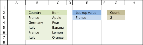
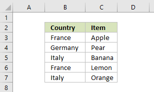
The array formula in cell G3 looks in column B for "France" and return adjacent values from column C. The array formula in cell G3 filters values unsorted, if you want to sort returning values alphabetically, read this:
Vlookup with 2 or more lookup criteria and return multiple matches
How to create an array formula
- Copy array formula above. (Ctrl + c)
- Double-press with left mouse button on a cell.
- Paste (Ctrl + v) array formula.
- Press and hold Ctrl + Shift simultaneously.
- Press Enter once.
- Release all keys.
Read more
How to enter an array formula | Convert array formula to a regular formula | How to enter array formulas in merged cells
The array formula above filters only values with one condition, the following article explains how to filter based on multiple criteria: Vlookup with 2 or more lookup criteria and return multiple matches
If you don't like array formulas, try this regular but more complicated formula in cell D10:
Explaining array formula (Return values vertically)
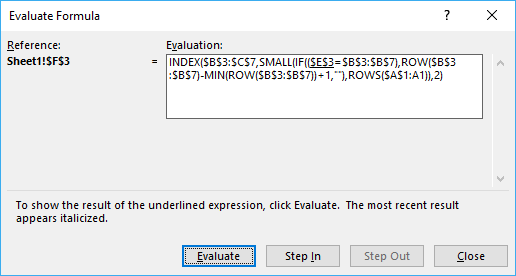
You can easily follow along as I explain the formula, select cell D10. Go to tab "Formulas" on the ribbon and press with left mouse button on "Evaluate Formula" button. Press with left mouse button on "Evaluate" button shown above to move to next step.
Step 1 - Identify cells equal to the condition in cell B10
= (equal sign) is a comparison operator and checks if criterion (E3) is equal to values in array ($B$3:$B$7). This operator is not case sensitive.
$B$10=$B$3:$B$7
becomes
"France"={"Germany";"Italy";"France";"Italy";"France"}
and returns
{FALSE, FALSE, TRUE, FALSE, TRUE}

The image above shows an array in cell range D3:D7 containing boolean values, those values correspond to the logical expression if cell B10 is equal B3:B7. Cell B5 and B7 is equal to cell B10, these return TRUE. The other remaining cells is not equal to cell B10 and return FALSE.
Step 2 - Create array containing corresponding row numbers
The ROW function returns the row number based on a cell reference, we are using a cell reference that points to a cell range containing multiple rows so the ROW function returns an array of row numbers.
MATCH(ROW($B$3:$B$7), ROW($B$3:$B$7))
The MATCH function finds the relative position of a value in a cell range or array, however, I am using multiple values so this step returns an array of numbers.
MATCH(ROW($B$3:$B$7), ROW($B$3:$B$7))
becomes
MATCH({3, 4, 5, 6, 7}, {3, 4, 5, 6, 7})
and returns {1,2,3,4,5}

The image above shows the array in cell range D3:D7, the array always begins with 1 and has must have the same number of values in the array as the table has rows.
Step 3 - Filter row numbers equal to a condition
The IF function has three arguments, the first one must be a logical expression. If the expression evaluates to TRUE then one thing happens (argument 2) and if FALSE another thing happens (argument 3).
IF(($B$10=$B$3:$B$7), MATCH(ROW($B$3:$B$7), ROW($B$3:$B$7)), "")
becomes
IF(FALSE, FALSE, TRUE, FALSE, TRUE}, MATCH(ROW($B$3:$B$7), ROW($B$3:$B$7)), "")
becomes
IF(FALSE, FALSE, TRUE, FALSE, TRUE},{1, 2, 3, 4, 5}, "")
and returns {"", "", 3, "", 5}

The IF function replaces the numbers that correspond to boolean value FALSE with "" (nothing) and boolean value TRUE with a number, shown in cell range D3:D7.
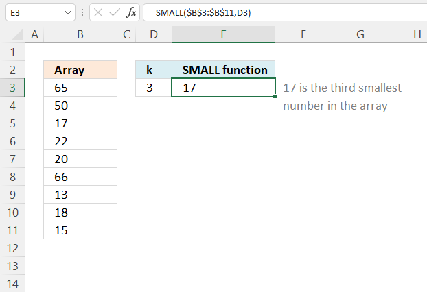
Step 4 - Return the k-th smallest row number
To be able to return a new value in a cell each I use the SMALL function to filter row numbers from smallest to largest.
The ROWS function keeps track of the numbers based on an expanding cell reference. It will expand as the formula is copied to the cells below.
SMALL(IF(($E$3=$B$3:$B$7),ROW($B$3:$B$7)-MIN(ROW($B$3:$B$7))+1,""),ROWS($A$1:A1))
becomes
SMALL({"", "", 3, "", 5}, ROWS($A$1:A1))
This part of the formula returns the k-th smallest number in the array {"", "", 3, "", 5}
To calcualte the k-th smallest value I am using ROWS($A$1:A1) to create the number 1.
When the formula in cell D10 is copied to cell D11, ROWS($A$1:A1) changes to ROWS($A$1:A2). ROWS($A$1:A2) returns 2.
The smallest number in array {"", "", 3, "", 5} is 3.
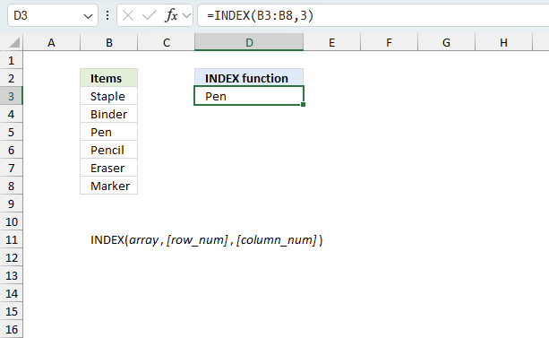
Step 4 - Return value based on row number
The INDEX function returns a value based on a cell reference and column/row numbers.
In Cell D10:
=INDEX($C$3:$C$7, 3)
becomes
=INDEX({"Pear", "Orange", "Apple", "Banana", "Lemon"}, 3)
and returns "Apple" in cell D10.
In Cell D11:
=INDEX($C$3:$C$7, 5) returns "Lemon"

This article demonstrates how to filter an Excel defined table programmatically based on a condition using event code and a macro.
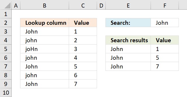
2. Return multiple values - case sensitive
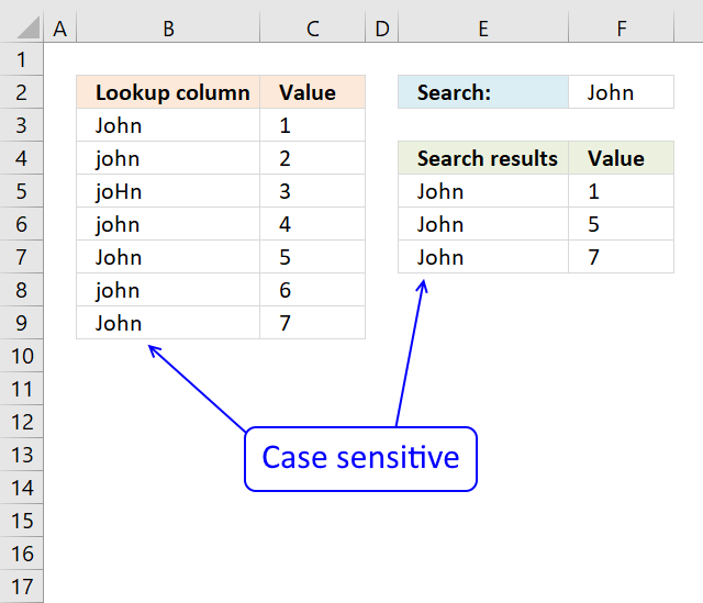
The array formula in cell F5 returns adjacent values from column C where values in column B matches the search value in cell F2 (case sensitive).
Excel 365 dynamic array formula in cell E5:
Here is the Excel 365 formula explained: Filter values based on a condition - case sensitive
The following array formulas are for earlier Excel versions.
Array formula in E5:
Array formula in F5:
Explaining array formula in cell E5
Step 1 - Check if values are an exact match to lookup value
The EXACT function checks if two values are precisely the same, it returns TRUE or FALSE. The EXACT function also considers upper case and lower case letters.
Function syntax: EXACT(text1, text2)
EXACT($B$3:$B$9, $F$2)
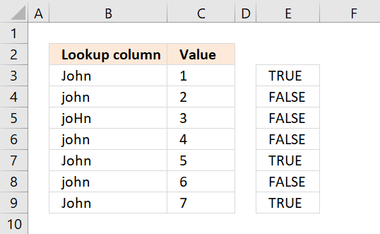
returns {TRUE; FALSE; FALSE; FALSE; TRUE; FALSE; TRUE}
The picture below shows the array in column E. TRUE means that the value in column B on the same row is identical to the lookup value.
Step 2 - Convert boolean array to row numbers if TRUE
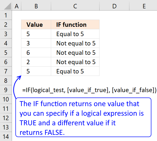
The IF function returns one value if the logical test is TRUE and another value if the logical test is FALSE.
Function syntax: IF(logical_test, [value_if_true], [value_if_false])
IF({TRUE; FALSE; FALSE; FALSE; TRUE; FALSE; TRUE},MATCH(ROW($B$3:$B$9), ROW($B$3:$B$9)), "")
becomes
IF({TRUE; FALSE; FALSE; FALSE; TRUE; FALSE; TRUE},{1;2;3;4;5;6;7}, "")
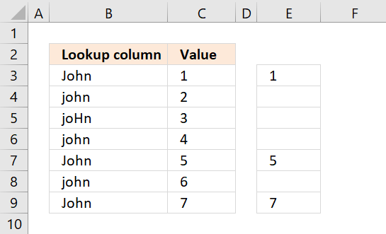
and returns {1;"";"";"";5;"";7}.
The picture below displays the array in column E. Now we know which rows the identical values have.
Step 3 - Extract the k-th smallest value from array
The SMALL function returns the k-th smallest value from a group of numbers.
Function syntax: SMALL(array, k)
SMALL(IF(EXACT($B$3:$B$9, $F$2),MATCH(ROW($B$3:$B$9), ROW($B$3:$B$9)), ""), ROWS($A$1:A1))
becomes
SMALL( {1;"";"";"";5;"";7}, ROWS($A$1:A1))
returns 1. Note that ROWS($A$1:A1) change when you copy the cell and paste to cells below. This makes the formula show all identical values.
Step 4 - Get value from cell range
The INDEX function returns a value or reference from a cell range or array, you specify which value based on a row and column number.
Function syntax: INDEX(array, [row_num], [column_num])
INDEX($B$3:$B$9, SMALL(IF(EXACT($B$3:$B$9, $I$2), MATCH(ROW($B$3:$B$9), ROW($B$3:$B$9)), ""), ROWS($A$1:A1)))
becomes
INDEX($B$3:$B$9, 1)
and returns John in cell E5.
Get excel *.xlsx file
Case sensitive vlookup and returning multiple values
3. Return multiple values - if not equal to

The picture above shows an array formula in cell C10 that extracts values from cell range C3:C7 if the corresponding value in cell range B3:B7 is NOT equal to the lookup value in cell B10.
The lookup value in cell B10 is not equal to the value in B3, B4, and B6. The corresponding values in C3, C4, and C6 are returned to cell C10 and cells below.
Array formula in cell C10:
Copy cell C10 and paste to cells below.
If you own Excel 365 you can use the much easier FILTER function to accomplish the same thing: Filter values if not equal to
4. Return multiple values - if smaller than

The image above demonstrates a formula in cell C10 that extracts items from cell range B3:B7 if the corresponding value in cell range C3:C7 is smaller than the value in cell B10.
In the example above, cells C5 and C7 are smaller than the value in cell B10. The corresponding cells are B5 and B7 which the formula returns in cell C10 and cells below.
Array formula in cell C10:
Copy cell C10 and paste to cells below.
If you own Excel 365 you can use the much easier FILTER function to accomplish the same thing: Filter values if smaller than
5. Return multiple values - if larger than

The picture above demonstrates a formula in cell C10 that extracts values from cell range B3:B7 if the corresponding values in C3:C7 are less than the value in cell B10.
In this example, cells C5 and C7 are smaller than the value in cell B10. The formula in cell C10 returns the corresponding values from B5 and B7.
Array formula in cell C10:
Copy cell C10 and paste to cells below.
If you own Excel 365 you can use the much easier FILTER function to accomplish the same thing: Filter values if smaller than
6. Return multiple values - if contains

The image above demonstrates a formula in cell C10 that extracts values from cell range C3:C7 if the corresponding values in cell range B3:B7 contain the value in cell B10.
In this example, the values in cells B3, B5, and B7 contain the value in cell B10. The array formula returns the corresponding values from cells C3, C5, and C7 to cell C10 and cells below as far as necessary.
Array formula in cell C10:
Copy cell C10 and paste to cells below.
If you own Excel 365 you can use the much easier FILTER function to accomplish the same thing: Filter values if contains
7. Return multiple values - if not contains

The picture above demonstrates a formula in cell C10 that extracts values from cell range C3:C7 if the corresponding values in cell range B3:B7 do not contain the value in cell B10.
In this example, the values in cells B4, and B6 do not contain the value in cell B10. The array formula returns the corresponding values from cells C4, and C6 to cell C10 and cells below as far as necessary.
Array formula in cell C10:
Copy cell C10 and paste to cells below.
If you own Excel 365 you can use the much easier FILTER function to accomplish the same thing: Filter values if contains
8. Return multiple values - that begins with

The formula in cell C10 extracts values from cell range C3:C7 if the corresponding values in B3:B7 begin with the same value as the value entered in cell B10.
The image above shows that cell B4 and B6 begins with the same value as the value in cell B10. The corresponding values in cell C4 and C6 are displayed in cell C10 and C11.
Array formula in cell C10:
Copy cell C10 and paste to cells below as far as needed.
If you own Excel 365 you can use the much easier FILTER function to accomplish the same thing: Filter values that begin with
9. Return multiple values - that ends with

Array formula in cell C10:
Copy cell C10 and paste to cells below as far as needed.
If you own Excel 365 you can use the much easier FILTER function to accomplish the same thing: Filter values that end with
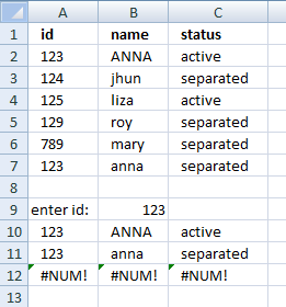
How to remove #num errors
The picture above shows you the array formula copied down to cell D12 however there are only two values shown, the remaining cells show nothing not even an error.
Array formula in cell D10:
The IFERROR function lets you convert error values to blank cells or really in whatever value you want. In this case it returns blank cells.
Recommended articles
How to use the IFERROR function | How to use the ISERROR function | How to use the ERROR.TYPE function | How to find errors in a worksheet | Delete blanks and errors in a list
10. Count matching values
The following image shows you a data set in column B and C. The lookup value in cell E3 is used for identifying matching cell values in column B.
Formula in cell G3:
Alternative formula in cell G3:
Recommended articles
Count a given pattern in a cell value | Count cells containing text from list | Count cells between specified values | Count entries based on date and time | Count unique distinct values | Count unique distinct records |
11. Return multiple values horizontally

Update 17 December 2020, use the FILTER function to return multiple values horizontally. Regular formula in cell C10:
The formula above works only in Excel 365. The array formula below is for earlier Excel versions and is entered in cell C10.
Array formula in C10:
Copy cell C10 and paste to cells to the right of cell C10 as far as needed.
Enter the formula above as an array formula or use this regular but more complicated formula:
Recommended articles
Search values distributed horizontally and return corresponding values | Resize a range of values | Rearrange values | Rearrange cells in a cell range to vertically distributed values | Rearrange values based on category(VBA) | Normalize data (VBA) | Normalize data, part 2 |
12. Extract multiple records based on a condition
Update 17 December 2020, use the new FILTER function to extract values based on a condition, formula in cell A10:
The FILTER function is available for Excel 365 users and the formula above is entered as a regular formula.
The formula below is for earlier Excel versions, it extracts records based on the value in cell B9. Array formula in cell A10:
To enter an array formula, type the formula in a cell then press and hold CTRL + SHIFT simultaneously, now press Enter once. Release all keys.
The formula bar now shows the formula with a beginning and ending curly bracket telling you that you entered the formula successfully. Don't enter the curly brackets yourself.
Copy cell A10 and paste to cell range B10:C10. Then copy A10:C10 and paste to cell range A11:C12.
3.1 Watch a video where I explain how to use the array formula and how it works
Enter the formula above as an array formula or use this regular but more complicated formula:
Recommended reading
- Extract all rows from a range that meet criteria in one column
- Match two criteria and return multiple records
- Extract records where all criteria match
- Search for a text string in a data set using an array formula
- Filter unique distinct records
13. Lookup and return multiple values [AutoFilter]
The AutoFilter is a built-in feature in Excel that allows you to quickly filter data. The following video shows you how to quickly filter a data set, I don't think you can do it more quickly than this.
13.1 Instructions on how to filter a data set [AutoFilter]
- Press with right mouse button on on a cell value that you want to filter
- Press with mouse on "Filter" and then "Filter by Selected Cell's Value"
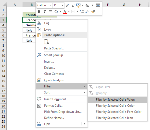
- That's it!
13.2 How to remove a filter
- Press with mouse on filter button next to header, shown in picture below
- Press with mouse on "Clear Filter From "Country""
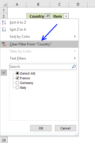
- The AutoFilter buttons next to each header are still there.
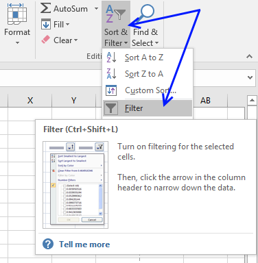
- If you want to remove those as well, go to tab "Home" on the ribbon and press with left mouse button on "Sort & Filter" button, then on "Filter"
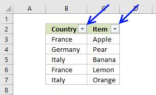
- The data set now looks like this:
14. Lookup and return multiple values [Advanced Filter]
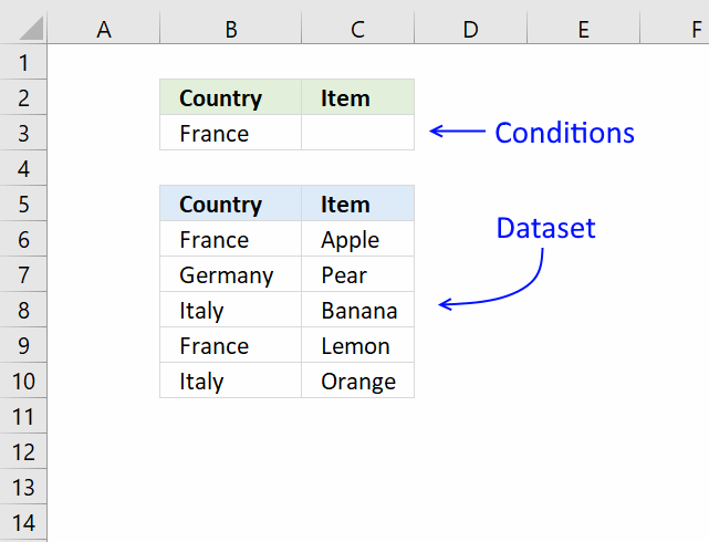
The Advanced Filter is a tool in Excel that allows you to filter a dataset using complicated criteria combinations like AND - OR logic that the regular AutoFilter tool can't accomplish.
In this case I am only going to filter based on a single condition so this will be an easy introduction to the Advanced Filter in Excel.
- Copy the dataset headers and place them above or below your dataset, this to avoid confusion if the conditions disappear when a filter is applied.
Rows will be hidden and if a condition is on the same row it will be hidden as well. I created headers on row 2, see image above. - Enter the condition below the correct header you want to apply a filter to, I entered my condition in cell B3.
- Select cell range B5:C10.
- Go to tab "Data" on the ribbon.
- Press with left mouse button on "Advanced" button.
- Press with left mouse button on in Criteria range: field and select cell range B2:C3
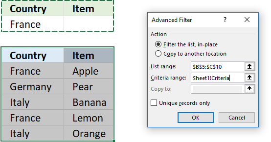
- Press with left mouse button on OK button.
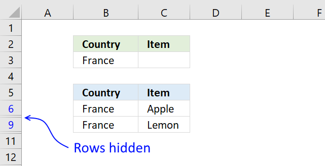
The image above shows the dataset filtered based on the condition used in cell B3. To clear the filter simply go to tab "Data" on the ribbon and press with left mouse button on "Clear" button.
15. Lookup and return multiple values [Excel Defined Table]
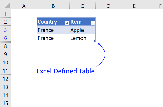
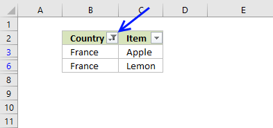
The image above shows you a dataset converted to an Excel Defined Table and filtered based on item "France" in column B.
- Select a cell in your data set.
- Press CTRL + T (shortcut for creating an Excel Defined Table).
- A dialog box appears, press with left mouse button on the checkbox if your data set contains headers.
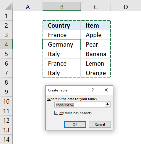
- Press with left mouse button on OK button.
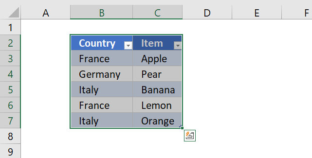
To filter the table follow these simple steps:
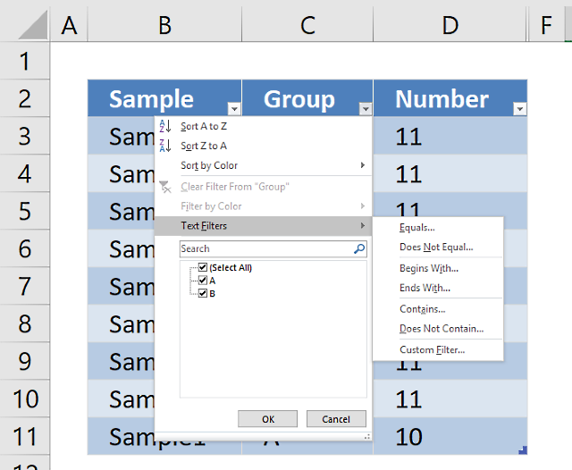
- Press with left mouse button on the black arrow next to a header name.
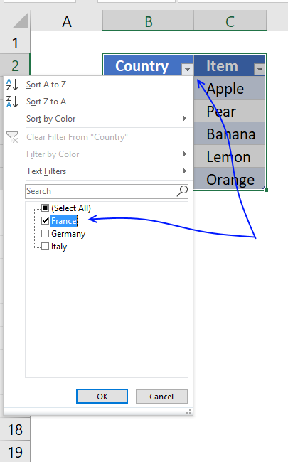
- Make sure the checkbox next to the value you want to use as a condition is selected.
- Press with left mouse button on OK button.
So why use an Excel defined Table? An Excel defined Table contains many more useful features.
- Enter a formula in one cell and Excel automatically enters the formula in the remaining Excel Table cells on the same column.
- Cell references are converted to structured references, for example a cell reference to column "Country" might look like this: Table[Country].
This is beneficial because you don't need to adjust cell references if your table grows or shrinks, the cell reference is the same no matter what. You don't need to use dynamic named ranges either. - Easy to filter and sort data.
- Easy to add or delete data, simply type your data below the last table row and the Excel defined Table will automatically expand.
- Use as data source for a chart and the chart will display what is filtered.
16. Return multiple values vertically or horizontally [UDF]

Make sure you have copied the vba code below into a standard module before entering the array formula.
16.1 User defined Function Syntax
vbaVlookup(lookup_value, table_array, col_index_num, [h])
16.2 Arguments
| lookup_value | Required. |
| table_array | Required. A cell reference to the data table you want to search. |
| col_index_num | Required. A number representing the column in the table_array. |
| [h] | Optional. Return values horizontally. |
Array formula in cell C14:D14:
16.3 Watch a video that explains how to use the User Defined Function
16.4 How to enter custom function array formula
- Select cell range C9:C11
- Type above custom function
- Press and hold Ctrl + Shift
- Press Enter once
- Release all keys
Recommended articles

Array formulas allows you to do advanced calculations not possible with regular formulas.
16.5 How to enter custom function array formula
- Select cell range C14:D14
- Type above custom function
- Press and hold Ctrl + Shift
- Press Enter once
- Release all keys
16.6 How to copy array formula to the next row
- Select cell range C14:D14
- Copy cell range
- Select cell range C15:D15
- Paste
16.7 Vba code
- Copy vba code below.
- Press Alt + F11 to open the visual basic editor.
- Press with right mouse button on on your workbook in the project explorer.
- Press with mouse on "Insert".
- Press with mouse on "Module".
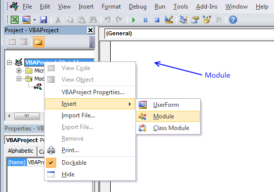
- Paste code to code module.
- Exit vb editor and return to Microsoft Excel
'Name User Defined Function and arguments
Function vbaVlookup(lookup_value As Range, tbl As Range, col_index_num As Integer, Optional layout As String = "v")

'Declare variables and data types
Dim r As Single, Lrow, Lcol As Single, temp() As Variant

'Redimension array variable temp
ReDim temp(0)

'Iterate through cells in cell range
For r = 1 To tbl.Rows.Count

   'Check if lookup_value is equal to cell value
   If lookup_value = tbl.Cells(r, 1) Then

      'Save cell value to array variable temp
      temp(UBound(temp)) = tbl.Cells(r, col_index_num)

      'Add anoher container to array variable temp
      ReDim Preserve temp(UBound(temp) + 1)
   End If
Next r

'Check if variable layout equals h
If layout = "h" Then

   'Save the number of columns the user has entered this User Defined Function in.
   Lcol = Range(Application.Caller.Address).Columns.Count

   'Iterate through each container in array variable temp that won't be populated
   For r = UBound(temp) To Lcol

       'Save a blank to array container
       temp(UBound(temp)) = ""

       'Increase the size of array variable temp with 1
       ReDim Preserve temp(UBound(temp) + 1)
   Next r

   'Decrease the size of array variable temp with 1
   ReDim Preserve temp(UBound(temp) - 1)

   'Return values to worksheet
   vbaVlookup = temp

'These lines will be rund if variable layout is not equal to h
Else

   'Save the number of rows the user has entered this User Defined Function in
   Lrow = Range(Application.Caller.Address).Rows.Count

   'Iterate through empty cells and save nothing to them in order to avoid an error being displayed
   For r = UBound(temp) To Lrow
      temp(UBound(temp)) = ""
      ReDim Preserve temp(UBound(temp) + 1)
   Next r

'Decrease the size of array variable temp with 1
ReDim Preserve temp(UBound(temp) - 1)

'Return temp variable to worksheet with values rearranged vertically
vbaVlookup = Application.Transpose(temp)
End If

End Function
17. VLOOKUP with 2 or more lookup criteria and return multiple matches
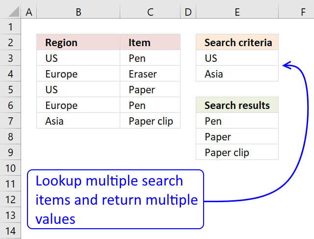
In this section I'll show you how to lookup two or more values in a list and return (if possible) multiple matches.
The picture above shows a table in column B and C, the search criteria is in column B and the results are in column G.
I am not using VLOOKUP at all in this array formula, the VLOOKUP looks for a value in the leftmost column of a table, and then returns a value in the same row from a column you specify.
The VLOOKUP function is not designed to look for multiple values and return multiple values.
Update, the new FILTER function is now available for Excel 365 users, formula in cell E7:
This formula is entered as a regular formula, read here how the formula works in detail: Filter values based on criteria
The formula below is for earlier Excel versions, array formula in E7:
How to enter an array formula
- Copy the aray formula above (Ctrl + c)
- Double press with left mouse button on cell G3
- Paste (Ctrl + v)
- Press and hold Ctrl + Shift simultaneously
- Press Enter
- Release all keys
If you made the above steps correctly the formula now has a beginning and ending curly bracket, like this:
{=array_formula)}
Don't enter these characters yourself, they appear automatically.
Recommended articles
Array formulas allows you to do advanced calculations not possible with regular formulas.
How to copy the formula to cells below
- Select cell E7
- Copy cell (Ctrl + c)
- Select cell range E8:E9
- Paste (Ctrl + v)
How the array formula works in cell E7
You can easily follow a long as I explain the array formula, get the workbook. Select cell B13, go to tab "Formulas". Press with mouse on "Evaluate formula" button.
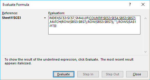
Press with mouse on "Evaluate" button show above to move to next step.
Step 1 - Count matching search criteria in column B
COUNTIF($E$3:$E$4, $B$3:$B$7)
returns {1;0;1;0;1}
Step 2 - Convert boolean array into corresponding row numbers
IF(COUNTIF($E$3:$E$4, $B$3:$B$7), MATCH(ROW($B$3:$B$7), ROW($B$3:$B$7)), "")
returns {1;"";3;"";5}
These are the row numbers that correspond to the matching values US and Asia in column B.
Recommended articles
Checks if a logical expression is met. Returns a specific value if TRUE and another specific value if FALSE.
Step 3 - Returns the k-th smallest row number
SMALL(IF(COUNTIF($E$3:$E$4,$B$3:$B$7), MATCH(ROW($B$3:$B$7), ROW($B$3:$B$7)), ""),ROWS($A$1:A1))
returns 1.
Recommended articles
The SMALL function lets you extract a number in a cell range based on how small it is compared to the other numbers in the group.
Step 4 - Return a value based on coordinate
INDEX($C$3:$C$7, SMALL(IF(COUNTIF($E$3:$E$4, $B$3:$B$7), MATCH(ROW($B$3:$B$7), ROW($B$3:$B$7)), ""), ROWS($A$1:A1)))
returns Pen in cell E7.
Recommended articles
Gets a value in a specific cell range based on a row and column number.
Get excel *.xlsx file
Vlookup with multiple search conditions and return multiple matches.xlsx
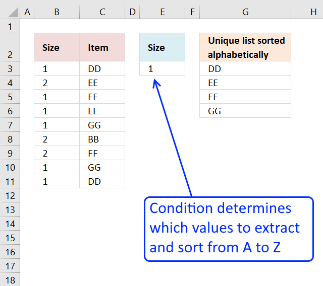
18. Extract multiple values based on a search value sorted from A to Z
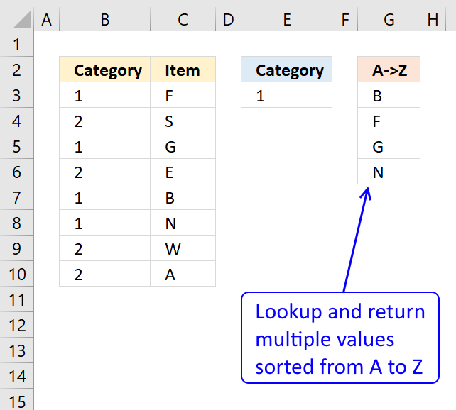
This example demonstrates a formula that works in most Excel versions. The formula in cell G3 extracts values from column C if the corresponding value on the same row matches the search value specified in cell E3.
The result is sorted from A to Z and displayed in cell G3 and cells below as far as needed.
Array formula in cell G3:
18.1 Watch a video where I explain the formula
Recommended article
Recommended articles
This article demonstrates how to extract unique distinct values based on a condition and also sorted from A to z. […]
18.2 How to enter an array formula
- Double press with the left mouse button on cell G3.
- Copy and paste the above formula to cell G3.
- Press and hold CTRL + SHIFT simultaneously.
- Press Enter once.
- Release all keys.
Take a look at the formula bar and you will see that the formula now has a beginning and ending curly bracket.
Don't enter these characters yourself, they appear automatically. Example, {=array_formula}
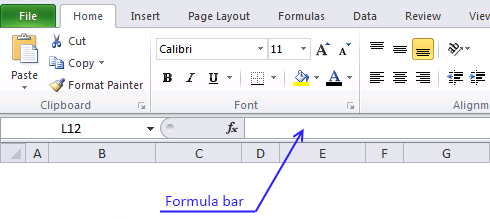
The image above demonstrates the location of the formula bar.
18.3 Explaining formula in cell G3
Step 1 - Sort values in column C
COUNTIF($C$3:$C$10, "<"&$C$3:$C$10)
returns {3;6;4;2;1;5;7;0}
Step 2 - Extract sort rank numbers for chosen category
IF($E$3=$B$3:$B$10, COUNTIF($C$3:$C$10, "<"&$C$3:$C$10), "")
returns {3;"";4;"";1;5;"";""}
Step 3 - Find k-th smallest value in array
SMALL(IF($E$3=$B$3:$B$10,COUNTIF($C$3:$C$10,"<"&$C$3:$C$10),""),ROWS($A$1:A1))
SMALL({3;"";4;"";1;5;"";""},1) and returns 1.
Step 4 - Match sort rank to find relative position
MATCH(SMALL(IF($E$3=$B$3:$B$10, COUNTIF($C$3:$C$10, "<"&$C$3:$C$10), ""),ROWS($A$1:A1)), COUNTIF($C$3:$C$10,"<"&$C$3:$C$10), 0)
becomes MATCH(1, {3;6;4;2;1;5;7;0}, 0) and returns 5.
Step 5 - Return values
INDEX($C$3:$C$10,MATCH(SMALL(IF($E$3=$B$3:$B$10,COUNTIF($C$3:$C$10,"<"&$C$3:$C$10),""),ROWS($A$1:A1)),COUNTIF($C$3:$C$10,"<"&$C$3:$C$10),0))
becomes INDEX($C$3:$C$10,5) returns B in cell G3.
Tip! You can easily filter values if you convert your data to an excel table and then sort them:
Recommended articles
An Excel table allows you to easily sort, filter and sum values in a data set where values are related.
19. Extract multiple values based on a search value sorted from A to Z (Excel 365)

This example demonstrates a regular formula that works only in Excel 365. The formula is a dynamic array formula in cell G3, it returns multiple values that spills to cells below automatically.
It contains two functions, the FILTER function and the SORT function. It extracts values from column C if the value on the same row in column B matches the search value specified in cell E3.
Formula in cell G3:
19.1 Explaining formula
Step 1 - Filter values based on a condition
The FILTER function extracts values/rows based on a condition or criteria.
FILTER(array, include, [if_empty])
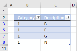
FILTER(C3:C10,E3=B3:B10)
returns {"F"; "G"; "B"; "N"}.
Step 2 - Sort result
The SORT function lets you sort values from a cell range or array.
SORT(array, [sort_index], [sort_order], [by_col])
SORT(FILTER(C3:C10,E3=B3:B10))
becomes
SORT({"F"; "G"; "B"; "N"})
and returns {"B"; "F"; "G"; "N"}.
20. Vlookup with multiple matches returns a different value
Linda asks in this post: How to return multiple values using vlookup in excel
I tried using the formula above but it didn't work for me and I can't figure out how to adjust it to accomodate my needs.
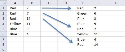
Here is what I have: Data Range is in $E$1:$F$8, I would like my results in Col. B. Lookup value in column A and return the value in Col F that matches.
Since there are duplicates in Col. A I want Col. B to return the next matching value from col. F.
Essentially this is a Vlookup with multiple matches that would return a different value. Thanks for any help you can provide.
Data Range Col. A Col B
Red 2 Red
Green 6 Red
Pink 3 Red
Blue 9 Yellow
Red 7 Blue
Yellow 11 Blue
Blue 4
Red 14
Answer:
Array Formula in cell B1:
How to enter an array formula
- Select cell B2
- Type the formula above
- Press and hold CTRL + SHIFT
- Press Enter
- Release all keys
If you did it right, the formula now has curly brackets before and after, like this: {=array_formula}.
Copy cell B1 and paste it down as far as needed.
Explaining formula in cell B1
Step 1 - Find value
A1=$E$1:$E$8
returns {TRUE; FALSE; ... ; TRUE}
Step 2 - Replace TRUE with corresponding row number
The IF function has three arguments, the first one must be a logical expression. If the expression evaluates to TRUE then one thing happens (argument 2) and if FALSE another thing happens (argument 3).
IF(A1=$E$1:$E$8, ROW($E$1:$E$8)-MIN(ROW($E$1:$E$8))+1, "")
returns {1;"";"";"";5;"";"";8}
Step 3 - Extract k-th smallest row number
To be able to return a new value in a cell each I use the SMALL function to filter row numbers from smallest to largest based on corresponding value.
SMALL(IF(A1=$E$1:$E$8, ROW($E$1:$E$8)-MIN(ROW($E$1:$E$8))+1, ""), COUNTIF(A1:$A$1, A1))
becomes
SMALL({1;"";"";"";5;"";"";8}, COUNTIF(A1:$A$1, A1))
The COUNTIF function counts values based on a condition or criteria, the first argument contains an expanding cell reference, it grows when the cell is copied to cells below. This lets the formula count values.
SMALL({1;"";"";"";5;"";"";8}, 1)
and returns 1.
Step 4 - Return value based on row number
The INDEX function returns a value based on a cell reference and column/row numbers.
INDEX($F$1:$F$8, SMALL(IF(A1=$E$1:$E$8, ROW($E$1:$E$8)-MIN(ROW($E$1:$E$8))+1, ""), COUNTIF(A1:$A$1, A1)))
becomes
INDEX($F$1:$F$8, 1)
and returns 2 in cell B1.
21. Lookup with multiple matches returns different values - Excel 365

This example shows a formula that performs a lookup based on the number of instances of a particular condition. This means that the formula returns a different value for each duplicate value corresponding to the data set.
Excel 365 formula in cell C3:
Explaining formula
Step 1 - Logical test
The equal sign is a logical operator that compares value to value, it is not case sensitive. The result is a boolean value TRUE or FALSE if the condition is met or not.
$E$3:$E$10=B3
returns {TRUE; FALSE; ... ; TRUE}.
Step 2 - Extract values based on a condition
The FILTER function extracts values/rows based on a condition or criteria.
Function syntax: FILTER(array, include, [if_empty])
FILTER($F$3:$F$10, $E$3:$E$10=B3)
returns {2; 7; 14}.
Step 3 - Count value across cells using a dynamic reference
$B$3:B3 is both an absolute and relative cell reference, $B$3 is absolute and B3 is a relative. This means that the cell reference grows when the cell is copied to cells below, it keeps track of how many instances of the current condition there are based on the cell and also the cells above the condition.
The COUNTIF function calculates the number of cells that is equal to a condition.
Function syntax: COUNTIF(range, criteria)
COUNTIF($B$3:B3, B3)
becomes
COUNTIF("Red", "Red")
and returns 1.
Step 4 - Get value
The INDEX function returns a value or reference from a cell range or array, you specify which value based on a row and column number.
Function syntax: INDEX(array, [row_num], [column_num])
INDEX(FILTER($F$3:$F$10, $E$3:$E$10=B3), COUNTIF($B$3:B3, B3))
returns 2.
22. Vlookup across multiple sheets
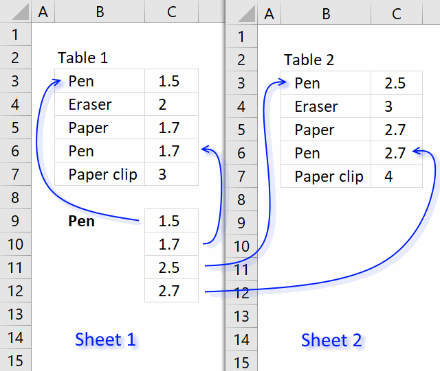
This section demonstrates two formulas, one for Excel 365 and one for earlier Excel versions. They search two tables on two different sheets and returns multiple results. Sheet1 contains table1 and sheet2 contains table 2.
The search value is Pen and is in cell B9, the formula finds two matches in sheet 1 row 3 and 6. It then continues to sheet 2 and finds two matches, row 3 and 6. The adjacent values from each match is returned to cell range C9 in sheet 1.
Array Formula in cell C9:
The following formula is an Excel 365 formula:
It spills values to cell C9 and cells below as far as needed. This Excel 365 formula is much smaller than the one for earlier versions, this shows clearly how far Excel has come the last years. Here is a breakdown:
VSTACK: This function stacks two or more arrays vertically. In this case, it's used twice.
- VSTACK(C3:C7, Sheet2!C3:C7): This stacks the values in cells C3:C7 from the current sheet (Sheet1) with the values in cells C3:C7 from Sheet2.
- VSTACK(B3:B7, Sheet2!B3:B7): This stacks the values in cells B3:B7 from the current sheet (Sheet1) with the values in cells B3:B7 from Sheet2.
- FILTER: This function filters the data based on a condition. In this case, the condition is:
- VSTACK(B3:B7, Sheet2!B3:B7) = Sheet1!B9
This means that the formula will only return the values from the stacked arrays where the value in the first stacked array (VSTACK(B3:B7, Sheet2!B3:B7)) matches the value in cell B9 on Sheet1. So, the entire formula can be read as:
"Filter the stacked values from columns C and B (from both Sheet1 and Sheet2) where the value in the stacked column B matches the value in cell B9 on Sheet1, and return the corresponding values from the stacked column C." In other words, the formula is looking for matches between the values in column B (across both sheets) and the value in cell B9, and then returning the corresponding values from column C.
Note that this formula is using the new dynamic array formulas in Excel 365, which allows for more flexible and powerful data manipulation. The FILTER function is one of the new functions introduced in Excel 365, and it's used here to filter the data based on the condition specified.
How to create an array formula
The following instructions are for earlier Excel versions than Excel 365.
- Copy (Ctrl + c) and paste (Ctrl + v) array formula into formula bar.
- Press and hold Ctrl + Shift.
- Press Enter once.
- Release all keys.
How to copy an array formula
The steps are for earlier Excel versions, ignore these if you are on Excel 365.
- Select cell C9
- Copy (Ctrl + c)
- Select cell range C9:C13
- Paste (Ctrl + v)
Explaining array formula (earlier Excel versions)
Step 1 - What values are equal to criterion?
The equal sign lets you create a logical expression that compares cell value in B9 with values in cell range B3:B7, it creates an array containing boolean values. TRUE or FALSE.
$B$9=$B$3:$B$7
becomes
"Pen"={"Pen"; "Eraser"; "Paper"; "Pen"; "Paper clip"}
and returns
{TRUE; FALSE; FALSE; TRUE; FALSE}
Step 2 - Convert array to row numbers
The IF function has three arguments, the first one must be a logical expression. If the expression evaluates to TRUE then one thing happens (argument 2) and if FALSE another thing happens (argument 3).
If the logical expression returns TRUE the IF function replaces those values with the corresponding row numbers, if FALSE it returns "" (blank).
IF(($B$9=$B$3:$B$7), ROW($B$3:$B$7)-MIN(ROW($B$3:$B$7))+1, "")
becomes
IF({TRUE; FALSE; FALSE; TRUE; FALSE}, ROW($B$3:$B$7)-MIN(ROW($B$3:$B$7))+1, "")
becomes
IF({TRUE; FALSE; FALSE; TRUE; FALSE}, {3; 4; 5; 6; 7}-MIN({3; 4; 5; 6; 7})+1, "")
becomes
IF({TRUE; FALSE; FALSE; TRUE; FALSE}, {3; 4; 5; 6; 7}-3+1, "")
becomes
IF({TRUE; FALSE; FALSE; TRUE; FALSE}, {1; 2; 3; 4; 5}, "")
and returns {1; ""; ""; 4; ""}
Step 3 - Return the k-th smallest row number
To be able to return a new value in a cell each I use the SMALL function to filter column numbers from smallest to largest. The SMALL function ignores text and blank values in the array which is very handy in this case.
SMALL(IF(($B$9=$B$3:$B$7), ROW($B$3:$B$7)-MIN(ROW($B$3:$B$7))+1, ""), ROW(A1))
becomes
SMALL({1; ""; ""; 4; ""}, ROW(A1))
becomes
SMALL({1; ""; ""; 4; ""}, 1)
and returns 1.
Step 4 - Return a value or reference of the cell at the intersection of a particular row and column
The INDEX function returns a value based on a cell reference and a row number and a column number if needed.
INDEX(tbl_1, SMALL(IF(($B$9=$B$3:$B$7), ROW($B$3:$B$7)-MIN(ROW($B$3:$B$7))+1, ""), ROW(A1)), 2)
becomes
INDEX(tbl_1,1, 2)

becomes
INDEX({"Pen", 1,5; "Eraser", 2; "Paper", 1,7; "Pen", 1,7; "Paper clip", 3},1, 2)
and returns $1,5
Step 5 - Return another value if expression is an error
The IFERROR function returns value_if_error if expression is an error and the value of the expression itself otherwise
IFERROR(value, value_if_error)
IFERROR function traps errors and starts looking for values in tbl_2
23. VLOOKUP a cell range and return multiple values
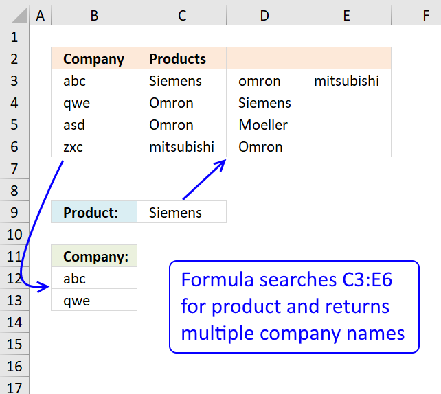
My database is as shown, where I have company abc sells siemens, omron and mitsubishi and company qwe sells omron n siemens.
Company Products
abc Siemens Omron Mitsubishi
qwe Omron Siemens
asd Omron Moeller
zxc Mitsubishi Omron
So right now I wanna key in the product name, lets say siemens, I hope it shows all the companies that sell siemens, in this case would be abc n qwe.
How is it possible? Using your formula can only works for first column, it will shows company abc only (first column), how to make it seach through the second column n show company qwe as well?
Answer:
This array formula looks up a value in a range (C3:E6) and returns multiple unique distinct values from a column (B3:B6). Cell C9 is the lookup value.
Excel 365 dynamic array formula in cell B12:
This array formula in cell B12 is for earlier Excel versions than Excel 365:
Watch a video where I explain how it works
How to create an array formula
- Double press with left mouse button on cell B12.
- Copy (Ctrl + c) and paste (Ctrl + v) above array formula to cell B12.
- Press and hold Ctrl + Shift simultaneously.
- Press Enter once.
- Release all keys.
How to copy array formula
- Select cell B12
- Copy (Ctrl + c)
- Select cell range B12:B14
- Paste ( Ctrl + v)
Explaining array formula in cell B12
Step 1 - Find matching values in array
($C$3:$E$6=$C$9)
returns {TRUE, FALSE, ... , FALSE}
Step 2 - Remove duplicate values in array
COUNTIF($B$11:B11, $B$3:$B$6)=0
returns {TRUE; TRUE; TRUE; TRUE}
Step 3 - Return row numbers
IF(($C$3:$E$6=$C$9)*(COUNTIF($B$11:B11, $B$3:$B$6)=0), ROW($C$3:$E$6)-MIN(ROW($C$3:$E$6))+1, "")
returns {1, "", "";"", 2, "";"", "", "";"", "", ""}
Step 4 - Find smallest row number
SMALL(IF(($C$3:$E$6=$C$9)*(COUNTIF($B$11:B11, $B$3:$B$6)=0), ROW($C$3:$E$6)-MIN(ROW($C$3:$E$6))+1, ""), 1)
becomes
SMALL({1, "", "";"", 2, "";"", "", "";"", "", ""}, 1)
and returns 1.
Step 5 - Return a value or reference of the cell at the intersection of a particular row and column
=INDEX($B$3:$B$6, SMALL(IF(($C$3:$E$6=$C$9)*(COUNTIF($B$11:B11, $B$3:$B$6)=0), ROW($C$3:$E$6)-MIN(ROW($C$3:$E$6))+1, ""), 1))
returns abc in cell B12.
24. VLOOKUP and return multiple values across columns

This section demonstrates a formula that lets you extract non-empty values across columns based on a condition. The image above shows the condition in cell B9 and the formula in cell range B10:B14.
The data set is in cell range A2:E7 and the lookup column is column A. The formula returns values from multiple rows if the corresponding value in the lookup column match, one value in each cell.
I geted the file lookup-vba3. I think I can use this to help me populate a calendar.I substituted dates for Pen, Paper, and Eraser. I then had locations substituted for $ values. Where I have a date of say, 11/27/12, I have 10 locations delivering that day.
Using the template as shown in the screenshot under "Return multiple values horizontally or vertically (VBA)".
I cannot expand past column "C" to return multiple values. I think it is in the array code but I cannot figure out how to return values past column C.
If you can help, greatly appreciated!
Thanks,
Jim
Answer:
Excel 365 dynamic array formula in cell B10:
Array formula in cell B10 for earlier Excel versions:
How to create an array formula
- Select cell B10.
- Press with left mouse button on in formula bar.
- Paste above array formula.
- Press and hold CTL + SHIFT simultaneously.
- Press Enter.
How to copy formula
- Select cell B10.
- Copy cell (Ctrl + c).
- Select cell range B11:B15.
- Paste (Ctrl + v).
The following array formula concatenates the returned values, the TEXTJOIN function is able to make the formula much smaller.
Array formula in cell B10:
Explaining array formula in cell B10
![]()
The INDEX function returns a value or a reference of the cell at the intersection of a particular column and row, in a given range.
INDEX($B$2:$E$7, row_num, column_num)
The first following three steps calculate the row_nums and the remaining steps calculate column_nums.
Step 1 - Find matching dates and non blanks
The equal sign is a logical operator. it lets you compare the value in cell B9 with cell range A2:A7, the logical expression returns TRUE if equal and FALSE if not.
$A$2:$A$7=$B$9
returns {TRUE; FALSE; ... ; TRUE}
The less than and greater than characters are also logical operators, they check if values in cell range B2:E7 are not blank.
$B$2:$E$7<>""
becomes
{"New York","Los Angeles",...,"San Francisco"}<>""
becomes
{TRUE, TRUE, ... , TRUE}
The parentheses allow you to manipulate the order of calculation which is really important in this step. The asterisk is a character that multiplies the two arrays, TRUE*TRUE = TRUE (1), TRUE*FALSE = FALSE (0) and FALSE * FALSE = FALSE (0). This means that AND logic is applied to the two arrays.
You can multiply arrays with different sizes as long as you follow certain rules, in this case, I am multiplying an array that has the same number of rows as the other array.
($A$2:$A$7=$B$9)*($B$2:$E$7<>"")
returns
{1, 1, ... , 0, 1}.
1 is the same as TRUE and 0 (zero) is FALSE. Excel converts the boolean values to their numerical equivalents when you perform arithmetic calculations between two or more arrays.
Step 2 - Return corresponding row numbers
IF(($A$2:$A$7=$B$9)*($B$2:$E$7<>""), MATCH(ROW($B$2:$E$7), ROW($B$2:$E$7)), "")
returns {1, 1, "", 1;... , 6}
Recommended articles
Checks if a logical expression is met. Returns a specific value if TRUE and another specific value if FALSE.
Step 3 - Return the k-th smallest value
SMALL(array, k)
SMALL(IF(($A$2:$A$7=$B$9)*($B$2:$E$7<>""), MATCH(ROW($B$2:$E$7), ROW($B$2:$E$7)), ""), ROW(A1))
becomes
SMALL({1, 1, "", 1;... , 6, "", 6}, 1)
and returns 1.
Recommended articles
The SMALL function lets you extract a number in a cell range based on how small it is compared to the other numbers in the group.
Step 1 - Find matching dates and non blanks
($A$2:$A$7=$B$9)*($B$2:$E$7<>"")
returns {1, 1, 0... , 1}
Step 2 - Calculate both row numbers and column numbers
IF(($A$2:$A$7=$B$9)*($B$2:$E$7<>""), MATCH(ROW($B$2:$E$7), ROW($B$2:$E$7))+1/MATCH(COLUMN($B$2:$E$7), COLUMN($B$2:$E$7)), "")
returns {2,1.5,"",... ,6.25}
Step 3 - Return the k-th smallest value
SMALL(array, k)
SMALL(IF(($A$2:$A$7=$B$9)*($B$2:$E$7<>""), MATCH(ROW($B$2:$E$7), ROW($B$2:$E$7))+1/MATCH(COLUMN($B$2:$E$7), COLUMN($B$2:$E$7)), ""), ROW(A1))
returns 1.25.
Step 4 - Subtract row numbers
SMALL(IF(($A$2:$A$7=$B$9)*($B$2:$E$7<>""), MATCH(ROW($B$2:$E$7), ROW($B$2:$E$7))+1/MATCH(COLUMN($B$2:$E$7), COLUMN($B$2:$E$7)), ""), ROW(A1))-SMALL(IF(($A$2:$A$7=$B$9)*($B$2:$E$7<>""), MATCH(ROW($B$2:$E$7), ROW($B$2:$E$7)), ""), ROW(A1))
returns 0.25
Step 5 - Calculate column number
1/(SMALL(IF(($A$2:$A$7=$B$9)*($B$2:$E$7<>""), MATCH(ROW($B$2:$E$7), ROW($B$2:$E$7))+1/MATCH(COLUMN($B$2:$E$7), COLUMN($B$2:$E$7)), ""), ROW(A1))-SMALL(IF(($A$2:$A$7=$B$9)*($B$2:$E$7<>""), MATCH(ROW($B$2:$E$7), ROW($B$2:$E$7)), ""), ROW(A1)))
becomes
1/0.25 and returns column number 4.
Final calculation in cell B10
The INDEX function uses the row and column number to determine which value to return.
IFERROR(INDEX($B$2:$E$7, SMALL(IF(($A$2:$A$7=$B$9)*($B$2:$E$7<>""), MATCH(ROW($B$2:$E$7), ROW($B$2:$E$7)), ""), ROW(A1)), 1/(SMALL(IF(($A$2:$A$7=$B$9)*($B$2:$E$7<>""), MATCH(ROW($B$2:$E$7), ROW($B$2:$E$7))+1/MATCH(COLUMN($B$2:$E$7), COLUMN($B$2:$E$7)), ""), ROW(A1))-SMALL(IF(($A$2:$A$7=$B$9)*($B$2:$E$7<>""), MATCH(ROW($B$2:$E$7), ROW($B$2:$E$7)), ""), ROW(A1)))), "")
becomes
IFERROR(INDEX($B$2:$E$7, 1, 4), "")
becomes IFERROR("Chicago", "") and returns "Chicago" in cell B10.
If the INDEX function returns an error value the IFERROR function catches the error and returns a blank "".
Vlookup and return multiple values category
Table of Contents Use a drop down list to search and return multiple values How to automatically add new items […]
Excel categories
748 Responses to “5 easy ways to VLOOKUP and return multiple values”
Leave a Reply
How to comment
How to add a formula to your comment
<code>Insert your formula here.</code>
Convert less than and larger than signs
Use html character entities instead of less than and larger than signs.
< becomes < and > becomes >
How to add VBA code to your comment
[vb 1="vbnet" language=","]
Put your VBA code here.
[/vb]
How to add a picture to your comment:
Upload picture to postimage.org or imgur
Paste image link to your comment.
Ok - I absolutely MUST comment on this! I've spent my entire day looking all over the web for help on doing a VLOOKUP to look up one value and return multiple corresponding values and have not found anything that has helped me as much as you have! =D You've made my day. Thank you for posting this!
~kenbra
I am happy you found this post, but my advice is to take a look at this post instead: Using array formula to look up multiple values in a list. It has an array formula not as complicated as this one.
Thank you for your comment!
I am trying to use your code for a calendar. the file template that you have shown I have opened. In place of the values in Column B, I would like to put dates. In Column C, for the $ values I would replace with addresses
When I try modifying the table and expanding it past three columns it tells me I am out of the array range.
Can you assist?
Thanks!
Jim,
Which formula and template?
Oscar,
I opened the file lookup-vba3.
I think I can use this to help me populate a calendar.
I substituted dates for Pen, Paper, and Eraser. I then had locations substituted for $ values.
Where I have a date of say, 11/27/12, I have 10 locations delivering that day. Using the template as shown in the screen shot under "Retun multiple values horizontally or vertically (vba)" I cannot expand past column "C" to return multiple values.
I think it is in the array code but I cannot figure out how to return values past column C.
If you can help, greatly appreciated!
Thanks,
Jim
Jim,
The function procedure can not return values from multiple columns.
This array formula returns values from a range, in cell B10:
I wish I could return all values to single a column.
Jim,
Now I know how to return all values to a single column.
Read this post:
Lookup and return multiple values from a range excluding blanks
Hi,
The formula here works great but I can't figure out how to change it to work with data in columns.
Here is what I have:
=INDEX(A2:E2,SMALL(IF(A1:E1=A3,COLUMN(A1:E1),""),COLUMN()))
A B C D E
1 A B A C D
2 Car Bus Aeroplane Rocket Ship
3 A
I'd expect the result to read:
A B
4 Car Aeroplane
...but instead I get
A B
4 #NUM #NUM
Can you offer any advice?
Rob,
In cell A4:
=INDEX($A$2:$E$2, SMALL(IF($A$1:$E$1=$A$3, COLUMN($A$1:$E$1), ""), COLUMN(A:A))) + CTRL + SHIFT + ENTER copied to the right as far as needed.
Thank you for your comment!
Thanks for your reply; again, this works a treat but when I try this with some of my own data in different cells I get an error. I assume this is due to the A:A reference at the end?
I've uploaded a screenshot here: https://tinypic.com/view.php?pic=j9brsk&s=6
This is an array formula, I think you forgot to press Ctrl + Shift + Enter.
See this blog post: https://www.get-digital-help.com/lookup-a-value-in-a-list-and-return-multiple-matches-in-excel/
In the top example, with data in vertical columns,is it possible to position the output horizontally (vs. vertically), next to the query?
RJW,
Yes, see this blog post: https://www.get-digital-help.com/lookup-a-value-in-a-list-and-return-multiple-matches-in-excel/
Oscar, on the first formula, any reason why you have multiplied with ))*(SEARCH(search_tbl, TRANSPOSE(INDEX(tbl, , 1, 1))))? As this step looks redunant?
Thanks!
I forgot this post.
Using countif() instead of search() reduces formula size.
The reason why I multiplied two search() in the first place, was to remove any cells that contained the search criteria, I was looking for exact matches.
Does anyone know how to do a vlookup of three columns to pull a single record?
Andy,
Can you elaborate?
Match a single criterion in any of three columns?
Match three different criteria in each column?
Match any of three different criteria in any column?
Andy,
See this post: https://www.get-digital-help.com/vlookup-of-three-columns-to-pull-a-single-record/
Hi. I used this formula and it works great. However I like to know how the formulas I use work. I have spent a lot of time on the internet trying to break it down but this one has me stumped. I understand part, like the VLOOKUP and INDEX but I don't know how the rest fits in. Are you able to break this down for the dummies? If you have time it would be greatly appreciated.
I used this and it worked great, except for it leaving #NUM! when there is no more data. I plan on having that formula copy and pasted 50 times so that when I add data to my list, it will come up properly. Is there anyway I can get excel to display a zero instead of #NUM! ?
nevermind, I just fixed it with a IF ISERROR thanks anyway though, great example and thanks for posting it
Do you suppose you could post that formula with the IF ISERROR parameters included?
Thanks
I figured it out. For those who were having problems with the #NUM value showing, here's the formula with the IF ISERROR parameters included:
=IF(ISERROR(INDEX($C$3:$C$16, SMALL(IF($B$21=$B$3:$B$16, ROW($B$3:$B$16)-MIN(ROW($B$3:$B$16))+1, ""), ROW(A1)))), "", INDEX($C$3:$C$16, SMALL(IF($B$21=$B$3:$B$16, ROW($B$3:$B$16)-MIN(ROW($B$3:$B$16))+1, ""), ROW(A1))))
This is for the initial formula addressing the initial question, not the subsequent modifications.
Thanks Rich!
Here is a shorter formula removing #num value
Excel 2003
=IF(ROWS($A$1:A1)>SUMPRODUCT(--($B$21=$B$3:$B$16)), "", INDEX($C$3:$C$16, SMALL(IF($B$21=$B$3:$B$16, ROW($B$3:$B$16)-MIN(ROW($B$3:$B$16))+1, ""), ROW(A1)))) + CTRL + SHIFT + ENTER
Excel 2007
=IFERROR(INDEX($C$3:$C$16, SMALL(IF($B$21=$B$3:$B$16, ROW($B$3:$B$16)-MIN(ROW($B$3:$B$16))+1, ""), ROW(A1))), "") + CTRL + SHIFT + ENTER
Hi,
Continuing your example, is there a way to "Eraser" and "Paper clip"? and keep goign down? It returns #NUM because Row is set to 3:3 after the two Pen entries. Is there a way to reset the row to ROW(1:1) after a new vlookup search string?
Thanks
Excel user, did you ever figure out how to accomplish this? I have been searching all over for this exact question and cannot find the answer. The equation works great but I need to use it thousands of times, and resetting the Row to 1:1 for every new search string is too cumbersome. Thanks.
Excel User,
I am not sure I understand but I think I covered your question in this post: https://www.get-digital-help.com/vlookup-with-2-or-more-lookup-criteria-and-return-multiple-matches-in-excel/
Great formula, and it ALMOST works for me. Unfortunately, I'm getting #num! in every cell. Here's what I'm trying to do: I have data in a1-h10. column c have dates in them. i want to enter a date in a13 and have it check column c for that date and have the entire row of those dates listed in a15-h25. I used your formula but changed the cells and i just get #num!. Here is the formula i used =INDEX($A$1:$H$10, SMALL(IF($A$13=$C$1:$C$10, ROW($C$1:$C$10)-MIN(ROW($C$1:$C$10))+1, ""), ROW()))
Please help. Thank you.
I also tried using your Extract-all-rows-that-contain-a-value-between-this-and-that-part-21 formula, and in every cell i get #ref!. I don't know what i'm doing wrong. please help.
Josh
Josh,
I think you are almost there.
Try this array formula in cell A15:
=INDEX($A$1:$H$10, SMALL(IF($A$13=$C$1:$C$10, ROW($C$1:$C$10)-MIN(ROW($C$1:$C$10))+1, ""), ROW(A1)), COLUMN(A1)) + CTRL + SHIFT + ENTER
Copy cell A15 and paste it into A15:H25.
They all say #num!? Am i missing a step or formatting?
Josh,
My formula works just fine here.
Maybe your date in A13 can´t be found in your date list in column C?
Check if your date list in column C has another date format than cell A13?
I'm using the first date in column C. They all still say #num!? Is it possible you send me an email and I can reply with the excel file as an attachment so you can take a look at it. This formula is the only thing remaining for me to start using this on a much bigger scale in another spreadsheet. It would really help me out. Thank you.
Josh
Josh,
You can email me, go to "Contact" on the website menu.
OK, I'm getting close! i used the formula in your Extract-all-rows-that-contain-a-value-between-this-and-that-part-21. I adjusted it so the 'and that' wasn't a factor and it only took values from 1 cell. I copied it to A15:H25. It populated all of A15:H25, but only with the first row that matched the date. there were 4 other rows that match the date, but it didn't enter them. here is the formula =IF(SUM(IF(($C$1:$C$10=$A$13), 1, 0))=ROW(), "", INDEX($A$1:$H$10, SMALL(IF(($C$1:$C$10=$A$13), ROW($C$1:$C$10), ""), ROW(A1)), COLUMN()))
is there something i need to add or remove?
Thank you again,
Josh
Thank you, Thank you, Thank you. I’m going to add the formula a few comments above to remove the #num! value. Thank you again.
Josh
Very helpful posts. I tried using the formula above but it didn't work for me and I can't figure out how to adjust it to accomodate my needs. Here is what I have: Data Range is in $E$1:$F$8
Data Range Col. A Col B
Red 2
Green 6
Pink 3
Blue 9
Red 7
Yellow 11
Blue 4
Red 14
Thank you for your very helpful posts. I tried using the formula above but it didn't work for me and I can't figure out how to adjust it to accomodate my needs. Here is what I have: Data Range is in $E$1:$F$8, I would like my results in Col. B. Lookup value in column A and return the value in Col F that matches. Since there are duplicates in Col. A I want Col. B to return the next matching value from col. F. Essentially this is a Vlookup with multiple matches that would return a different value. Thanks for any help you can provide.
Data Range Col. A Col B
Red 2 Red
Green 6 Red
Pink 3 Red
Blue 9 Yellow
Red 7 Blue
Yellow 11 Blue
Blue 4
Red 14
Linda,
read this post: Vlookup with multiple matches returns a different value in excel
looking for a formula that will take a part number from one column and go and look for all related vehicle applications per that part number and return the vehicle applications to a single cell related back to the part number
Oscar,
Recently found your site and find the examples and information absolutely wonderful. Wish I had found your site earlier. I am currently designing a spreadsheet and require to do a lookup where I am matching two values and displaying a third. I am required to look up a Sales persons name and discount rate used for particular clients and return the clients Account number.
This is the formula I have come up with so far =INDEX($M$3:$M$14, SMALL(IF(AND($P$5=$K$3:$K$14,$P$4=$L$3:$L$14), ROW($K$3:$K$14)-MIN(ROW($K$3:$K$14))+1, ""), ROW(A1)))
This is only a little test example I have been working on the main spreadsheet is a lot larger with the values spread apart by 20 or more columns. Any suggestions you have would be greatly appreciated.
Thanks in advance
Scott Everist,
=INDEX($M$3:$M$14, SMALL(IF(($P$5=$K$3:$K$14)*($P$4=$L$3:$L$14), ROW($K$3:$K$14)-MIN(ROW($K$3:$K$14))+1, ""), ROW(A1))) + CTRL + SHIFT + ENTER.
HI,
Thanks for the same.
I Tried a lot but i didnt get. i want to know how to use the same.
Please requesting you kindly help me on this.
Regards,
Chandra
Chandra,
Did you get the excel example file?
Hi there, I think I understand the logic behind these formula but when I try to amend it it doesn't work. I got the example file.
This formula below works
INDEX(tbl,SMALL(IF($E$8=$B$2:$B$6,ROW($B$2:$B$6)-MIN(ROW($B$2:$B$6))+1,""),ROW(A1)),2)
Originally tbl is referencing B2:C6
I change it so that it is referencing B2:D6
Pen $1.50 Red
Eraser $2.00 Blue
Paper $1.00 Green
Pen $1.70 Yellow
Paper clip $3.00 Black
and then update the formula to
INDEX(tbl,SMALL(IF($E$8=$B$2:$B$6,ROW($B$2:$B$6)-MIN(ROW($B$2:$B$6))+1,""),ROW(A1)),3)
I would expect 'Red' and 'Yellow' to be returned instead of 1.50 and 1.70 but instead the formula will not calculate.
Any suggestions?
Ignore last. Realised it was because I hadn't pressed CTRL + SHIFT + ENTER!
Thanks very much for your post. It has really helped me!
Ignore last. Realised I hadn't hit CTRL + SHIFT + ENTER!
Thanks for your post. It really helped me.
hi,
i have two workook...1st workbook is called the master sheet and the second is new workbook where in i had to filter out the data that i require in the new workbook and then i have to copy and paste into the master sheet that is the 1st workbook..could u please suggest me
Can you describe your problem in greater detail?
Richard,
Read this post: Excel udf: Lookup and return multiple values concatenated into one cell
Oscar:
So thankful to have found this formula. I modified it slightly so that results are provided horizontally in the same row rather than vertically. The formula works great in the 1st row, but when I try to copy it down to subsequent rows, it keeps giving me the same output as the 1st row. Can you help? Here is the formula I'm using:
{=INDEX(Results!$B$1:$B$4372, SMALL(IF(Results!$A$1:$A$4372=$A$1, ROW(Results!$A$1:$A$4372)-MIN(ROW(Results!$A$1:$A$4372))+1, ""), COLUMNS($A:A)))}
This is just awesome. Thank you. Had to do a big tweek to do a less than if statement. But wow this worked great. Thank you
Greg,
True, all matching values are returned (Results!$A$1:$A$4372=$A$1) horizontally.
When you copy your formula to the next row, nothing changes. The same values are returned.
What values are you looking for, in row two?
Values filtered with another criterion, Results!$A$1:$A$4372=$A$1?
Or adjacent values to Results!$B$1:$B$4372?
Joe,
Thanks for your comment!
I believe values filtered with another criterion - the criterion in A2, then A3, then A4...with all matches for A2 placed in B2, all matches for A3 placed in B3...
The data sheet ("Results") I'm pulling from has 2 columns:
ART101 The professor was great!
ART101 There was too much work in this class.
ART101 Learned a lot.
ART333 Good class.
ART333 Loved the lectures.
The sheet I'm trying to create: all comments for a given course placed in the same (1) row, each comment in a new column. So...
ART101 The professor was great! There was too much work...
ART333 Good class. Loved the lectures.
Greg,
Try =INDEX(Results!$B$1:$B$4372, SMALL(IF(Results!$A$1:$A$4372=$A1, ROW(Results!$A$1:$A$4372)-MIN(ROW(Results!$A$1:$A$4372))+1, ""), COLUMNS($A:A))) + CTRL + SHIFT + ENTER
Presto! Wish I had found you earlier & saved so many hours! Thanks so much for lending your expertise.
Greg
=INDEX(Sheet1!$B$2:$B$30102,SMALL(IF((Sheet1!$L$2:$L$30102>=$Q$1)*
(Sheet1!$L$2:$L$30102<=$Q$2),ROW(Sheet1!$B$2:$B$30102)),ROWS($1:1)))
Where
B=Region
L=Target Start Date (ranging from early 2005 and still growing)
Q1&Q2 are start/end dates to narrow the field for L
The problem i am finding is that many of our earlier entries (mostly from 2005-2008, but found even in january 2011) do not have a target start date. With that said, I am unable to narrow my search by start/end date (q1/q2) b/c the query returns all entries w/o target start dates first (1/0/1900...there are thousands of these that I DO NOT NEED).
How can i modify this query to eliminate blank cells or ONLY return the dates that i specify (q1/q2)?
Thanks in advance!!!
Don,
=INDEX(Sheet1!$B$2:$B$30102,SMALL(IF((Sheet1!$L$2:$L$30102>=$Q$1)*
(Sheet1!$L$2:$L$30102<=$Q$2),ROW(Sheet1!$B$2:$B$30102)),ROWS($1:1))) ROW(Sheet1!$B$2:$B$30102) returns this array: (2, 3, 4, 5, ... , 30102) I think you want it to return this array: (1, 2, 3, 4, ... , 30101) So the formula becomes: =INDEX(Sheet1!$B$2:$B$30102,SMALL(IF((Sheet1!$L$2:$L$30102>=$Q$1)*
(Sheet1!$L$2:$L$30102<=$Q$2),ROW(Sheet1!$B$2:$B$30102)-MIN(ROW(Sheet1!$B$2:$B$30102))+1),ROWS($1:1))) or this: =INDEX(Sheet1!$B$2:$B$30102,SMALL(IF((Sheet1!$L$2:$L$30102>=$Q$1)*
(Sheet1!$L$2:$L$30102<=$Q$2),ROW(Sheet1!$B$1:$B$30101)),ROWS($1:1))) So why use: ROW(Sheet1!$B$2:$B$30102)-MIN(ROW(Sheet1!$B$2:$B$30102))+1 If you have named ranges instead of absolute cell references, the formula automatically adjusts to whatever cell range you select in the "Name Manager". Now, you question. Try this formula: =INDEX(Sheet1!$B$2:$B$30102, SMALL(IF((Sheet1!$L$2:$L$30102<>"")*(Sheet1!$L$2:$L$30102>=$Q$1)*
(Sheet1!$L$2:$L$30102<=$Q$2), ROW(Sheet1!$B$2:$B$30102)-MIN(ROW(Sheet1!$B$2:$B$30102))+1), ROWS($1:1)))
I definitely underdstand where my logic was flawed with the original formula. Thanks for the correction!!!
Unfortunately, the new formula:
=INDEX(Sheet1!$B$2:$B$30102, SMALL(IF((Sheet1!$L$2:$L$30102"")*(Sheet1!$L$2:$L$30102>=$Q$1)*
(Sheet1!$L$2:$L$30102<=$Q$2), ROW(Sheet1!$B$2:$B$30102)-MIN(ROW(Sheet1!$B$2:$B$30102))+1), ROWS($1:1)))
is still yielding blank cells (which will always occur due to departmental error). I need to accurately account for data between certain date ranges going back as far as 20005, but am unable due to these blank cells (which are contracts that might or might not be billed at a later date, so removal is not a possibility).
Do you have any other suggestions how I can avoid having blank cells return within this query?
Thanks in advance for your help, you are a lifesaver!!!!
I copied down the formula wrong in my last reply, but the formula:
=INDEX(Sheet1!$B$2:$B$30102, SMALL(IF((Sheet1!$L$2:$L$30102"")*(Sheet1!$L$2:$L$30102>=$Q$1)*
(Sheet1!$L$2:$L$30102<=$Q$2), ROW(Sheet1!$B$2:$B$30102)-MIN(ROW(Sheet1!$B$2:$B$30102))+1), ROWS($1:1)))
does still query blank cells. Sorry for the confusion.
It isn't allowing the two arrows to copy over from my computer to this thread (the ones after the first $L30102, where i assume you are trying to avoid the blank cells). Sorry for the multiple responses, just want to avoid confusion.
Don,
I recreated your problem and tried my formula. It works here. Are you sure the empty cells in Sheet1!$L$2:$L$30102 are empty?
yes, they are empty (as far as i can tell) and yield a 1/0/1900 result when returned through a query.
The problem might be that "Sheet1!" is pulling data from an Access database directly. Could this cause a problem? I can't alter the access data as it is utilized by various departments within my company, which is why i had the data pushed to the excel spreadsheet (i can refresh the data as often as i like).
Is there any way to modify this formula to specify dates w/in the formula, instead of using specified cells? I say this b/c when i use a sumproduct formula
=SUMPRODUCT((Sheet1!$L$2:$L$30072>=DATE(2011,1,15))*(Sheet1!$L$2:$L$30072<=DATE(2011,1,21))*((Sheet1!$B$2:$B$30072=$A$20)*(Sheet1!$AI$2:$AI$30072=$A23)))
it, obviously doesn't return any 1/0/1900......can we do this with an index? Or can you think of another way to avoid the 1/0/1900 error?
Don,
If I format an empty cell as Date, the cell returns nothing.
If I format an cell containing 0 as Date, the cell returns 1-0-1900.
Try this formula:
=INDEX(Sheet1!$B$2:$B$30102, SMALL(IF((Sheet1!$L$2:$L$30102<>0)*(Sheet1!$L$2:$L$30102>=$Q$1)*
(Sheet1!$L$2:$L$30102<=$Q$2), ROW(Sheet1!$B$2:$B$30102)-MIN(ROW(Sheet1!$B$2:$B$30102))+1), ROWS($1:1)))
For the life of me I cannot get this to work on my spreadsheet. So frustrating.
Jim,
Post your formula here and I´ll see what I can do.
Thanks very much for this help. The information is very well presented and explanied.
I am attemting to do what is described above however rather than actually listing the mutiple values in different cells I just want to add them all together and find the total in one cell. Do you know if this is possible or is there an easy method.
Thanks
Henry
Henry Nichols,
SUMIF(range, critera, [sum_range])
Adds the cells specified by a given condition or criteria.
HI,
Nice one, just a little mistake
Here is the correct one
=INDEX($C$2:$C$6, SMALL(IF($B$8=$B$2:$B$6, ROW($B$2:$B$6)-MIN(ROW($B$2:$B$6))+1, ""), ROW($A$1:$A$6)))
At the end it is not Row(A1), but has to be a vector for an increasing increment.
cybou,
It is not a mistake, ROW(A1) is a relative cell reference.
Get the example file and check it out.
Hi Oscar et al, need your help, I'm using excel 2003. This is my problem.Sheet 1 COL A contains fruits, col B to H contains there prizes daily (1 week). take note that in col. A fruits name may randomly repeated in col A. What I need is put in Sheet 2 col A all fruit name but not repeated and put to column B to H, I to N, O to U there prizes .see sample below. hope u understand.
A B C .... I
1 apple 10 11 .... 8
2 orange 9 9 ..... 10
3 apple 11 11 ..... 12
4 apple 14 10 ..... 10
5 grapes 15 15 ..... 14
In sheet 2 answer should be like this.
A B C ..... H I J.....N O P.... U
1 apple 10 11 8 11 11 12 14 10 10
2 orange 9 9 10
3 grapes 15 15 14
tHANKS
this was like returning multiple values, but in a columns not in a row....
john,
read this post: Merge matching rows in excel
Hi Oscar, that's was great, but one thing I'd noticed, it was arranged ascending, i think due to =small(), i'd tried to omit small but it failed on the second batch of lookup value e.g. apple.
by the way, i used this formula to get unique values on col A.
=if(countif($A$2:A2,A2)=A2,""), then I copy all return values except blank after filtering, :)...
john,
Yes, it is arranged ascending. The array formula would be complicated and large if I had implemented all your requirements. I think it is much easier to create an user defined function to solve your question.
john,
I have uploaded a new excel file to blog post: Merge matching rows in excel
Sheet 3 contains values, not arranged. The downside is the array formula is a lot more complicated. I created named ranges to minimize formula size.
A big thanks Oscar, I got the file and will try to understand that..you're awesome...keep up...
I like this - but would like the #num not to be displayed if the value is not found. Sometimes I have 3 values and at other times may be 5
Elwil,
IFERROR() function filters errors.
Just wanted to say thanks, what an awesome bit of excel-ing
You are most welcome! Thanks for commenting!
Oscar,
Thanks-- I'm using Excel 2003 and used the VLookup array successfully. However I'm been unsuccessful adding the IFERROR() function to clean up the sheet. Could you provide further explanation on using IFERROR for Excel 2003.
IFERROR is a function in excel 2007 and later versions.
Excel 2007
IFERROR(value, value_if_error)
Excel 2003 and earlier versions:
IF(ISERROR(formula), value_if_error, formula)
Hi,
First off thanks for the help ur site is great.
My question is in addition to the formula mentioned is there any way I can get the formula to return unique values only?
For the example above, if Pen had 4 prices ($1.5,$1.7,$1.5 and $1.7) is there a way to get only one 1.5 and 1.7?
I hope my question is clear...
Thanks!
Gi99a,
In my blog post example above, array formula in cell C8:
=INDEX(tbl, SMALL(IF(($B$8=$B$2:$B$6)*(COUNTIF($C$7:C7, $C$2:$C$6)=0), ROW($B$2:$B$6)-MIN(ROW($B$2:$B$6))+1, ""), ROW(A1)), 2) + CTRL + SHIFT + ENTER.
Hey,
Thanks for ur reply.
However this still gives me all values of "pen" so cell C8 onwards would give me repeated values for pen if there are any in "tbl"...
Gi99a
Get the example file
When I change the data of the above example as below, it cannot output correctly. Could you solve it?
-------------------------
Data:
Pen $1.50
Pen $1.50
Pen $5.00
Pen $18.00
Paper clip $3.00
Output:
Pen $1.50
$18.00
#NUM!
-------------------------
AY,
You are right! I uploaded a new file. Thanks for commenting!
I'm not even sure if this website is still active or if you would even receive this message but I will ask anyways!
I am needing to produce the same results that Gi99a needed but is there a way to produce them in a single cell instead of down the column?
Thanks in advance!
Hi,
I understand the formula very well. The only issue im having is that when I press Ctrl-shift-enter, the array works but the row(a1) part and any variation of it doesnt change. Meaning that instead of becoming a1,a2,a3 ... it is a1,a1,a1 and it makes sense because the positions I get when I tested it was 373,373,373 always giving me the same index.
Please help, thx
-Stefan
Hi,
Nevermind figured out my issue, but I will leave it here in case anyone else will have the same issue. I used column() at the end of the formula instead of column(a1). This will give you the number of the current column though so you will have to adjust by adding or subtracting.
Thx,
Stefan
Stefan,
How to use this array formula:
1. Type:
in cell B25.
2. Press CTRL + SHIFT + ENTER
3. Select cell B25
4. Copy cell B25. (Ctrl + c)
5. Paste it to the cells below as far as needed. (Ctrl + v)
If you don´t follow these instructions, the relative cell reference in ROW(A1) won´t change and will use cell reference a1 in all cells.
Hello Oscar,
LOVE this example, my issue/need is, I need to add the results. So instead of States and Names, I have to match a client name, and add all the sales totals:
clientA 10
clientA 10
clientA 10
clientB 5
clientB 5
clientB 5
So if I search for clientA, I need one cell that keeps a running total as sales are added. Lastly, a date range will need to be given, so search for sales from clientA between two dates and keep a running total...
Any chance you could help me out?
Thank you so much!!
~Andrew
Andrew,
Read: Running totals within date range in excel
Thanks for a great question!
Thank you for this, it was really helpful.
ErikB,
Thanks for your comment, I appreciate it!
How to return multiple values using vlookup in excel and removing duplicates?
my sheet is setup as follows
A B C D E
1 Section Category item flavor size
2 food Coffee Espresso none Single
3 food Coffee Espresso none double
4 food Coffee Americano none Single
5 food Coffee Americano none double
i have tried the formula to return multiple values using the index example and worked fine with none duplicate item but how can i list them without the duplicate?
appreciate your help
Ahmed Ali,
Read this post: Vlookup – Return multiple unique distinct values in excel
Hello Oscar,
I tried the formulas couple times and they do not work. I want Vlookup to add all the group A $ and placed on Sheet2 group A. For example:
Sheet1:
GRP $
A 2
A 2
A 2
B 3
B 3
B 3
C 4
C 4
C 4
Sheet2:
Grp $
A ???
B ???
C ???
if I add manually group A total is $6 and B total is $9 and C total is $12.
Thank you very much,
newsuteuser2011
newsiteuser2011,
or create a pivot table on sheet2
Oscar, what happen if I need to use IF(ISERROR(Vlookup)) and the datas are pretty big for every month. Is there a way to request Vlookup to pickup more than the first data?
Thank you,
Newsiteuser2011
newsiteuser2011,
Try the formula in this post: How to return multiple values using vlookup in excel
Oscar,
I am trying to use your formula and adjust it so that more rows can be selected, but get a #VALUE error. I've changed the references to include more than 16 rows, but then I get the error. Here is the equation:
=INDEX($C$3:$C$20,SMALL(IF($H$3=$B$3:$B$20,ROW($B$3:$B$20)-MIN(ROW($B$3:$B$20))+1,""),ROW(A4)))
All that seems to have changed is extending the array and search parameters. Can you help? I like what you have done and it seems to be ingenious. Thanks!
-S
Sim,
try:
=INDEX($C$3:$C$20,SMALL(IF($H$3=$B$3:$B$20,ROW($B$3:$B$20)-MIN(ROW($B$3:$B$20))+1,""),ROW(A1)))
ROW(A1) contains a relative cell reference, when you copy the cell (not the formula!), the relative cell reference changes.
Oscar,
Using the formula above still gives me the #Value error - and I noticed this. When I try to edit the formula in the formula bar, even if I make no changes, just put the cursor there and then get out, it changes from a functional formula to a #Value error. The {} at either end of the formula disappear and when I try to reinsert them, it just gives me this formula in the field:
{=INDEX($C$3:$C$16,SMALL(IF($H$3=$B$3:$B$16,ROW($B$3:$B$16)-MIN(ROW($B$3:$B$16))+1,""),ROW(A1)))}
Am I missing a formatting issue?
Sim,
It is an array formula.
How to create an array formula
Copy (Ctrl + c) and paste (Ctrl + v) array formula into formula bar.
Press and hold Ctrl + Shift.
Press Enter once.
Release all keys.
Hey there, I'd just like to drop a bomb of thanks, this helped reduce my fear of ARRAY formulas man. This post was a BIG help!
Dear Oscar,
First of all thank you for sharing your expertise in excel. I am one who benefited from all your comments and formula here. I have some difficulties though from the below formula. Basically I'm using xcelsius 2008, and the problem is ROW function is not recognize by xcelsius, can please help me with the same concept of the below formula without using the row function? I'm using the below formula because i want the multiple results using vlookup. please help. Thanks
Marlon
=VLOOKUP($Y$1, INDEX($AA$38:$AO$51, SMALL(IF($Y$1=INDEX($AA$38:$AO$51, , 1), ROW($AA$38:$AO$51)-MIN(ROW($AA$38:$AO$51))+1, ""), ROW(7:7)), , 1), $AB$36, FALSE)
Marlon,
Sorry, I have no knowledge about xcelsius 2008.
Awesome work Oscar,
I just have one question, i'm using this formula:
=IF(INDEX(Contactos!$CI$2:$CI$2445;SMALL(IF(Contactos!$CE2=Contactos!$CE$2:$CE$2445;ROW(Contactos!$CE$2:$CE$2445)-MIN(ROW(Contactos!$CE$2:$CE$2445))+1; ""); ROW($A$1)))=AP$1;"X";"") + CTRL + SHIFT + ENTER
My excel is similar to this:
A B C D E F
Names
And in the $CI$2:$CI$2445 range, there are some repeated names, this formula only populates one (A B C D E F), the first it finds, how can i put this to populate more ?
Thanks!
Rui Costa,
Thanks!
Can you describe what the formula is supposed to do in greater detail?
I'm using Excel 2007 and I have 2 Sheets:
Sheet1:
____A B C D E F
bla X X X
ble X X
Sheet2:
Name Letter1 Letter2
bla___A______B
ble___A______C
bla___B______A
I'm trying to make a formula to put in the cell where is the first X after bla, that checks the Sheet 2 for name and populates with the X the letters it finds..
Rui Costa,
read this post: Merge matching rows in excel (text values)
Hi.This array formula is great job and works fine for me,but when cell is empty it give's me an error #NUM.How do i stop this error?These cells need to be fill in later in a month.
Thanks.
Hi Oscar, great explaination!!!
I am having a scenario here, lets say I have a company list who sell many brands of products.
Company Products
abc Siemens Omron Mitsubishi
qwe Omron Siemens
asd Omron Moeller
zxc Mitsubishi Omron
I would like to key in the product, then it shown relevant companies. The example shown is great for my first column of products. But for the whole array how is it gonna works?
Thank you
Tony R,
Excel 2007, remove #NUM:
wackyboy,
I am not sure I understand. I think this post has an answer for you:
Merge matching rows in excel (text values)
Hi Oscar,
I am not looking for merging match rows.. My database is as shown, where I have company abc sells siemens, omron and mitsubishi and company qwe sells omron n siemens. So right now I wanna key in the product name, lets say siemens, I hope it shows all the companies that sell siemens, in this case would be abc n qwe. How is it possible? Using your formula can only works for first column, it will shows company abc only (first column), how to make it seach through the second column n show company qwe as well?
Thank you so much.
Duuuude, you have no idea how helpful this was
Munir,
thanks!
wackyboy,
read this post: Vlookup a range in excel
Hi Oscar,
I am trying to implement this formual in my spreadsheet but it is just returning the first row and the rest of the rows are #num.
I have data in A2:B602. I entered the name to look up in cell c2. I want it to return all the data corresponding to that name in column D. Could you please suggest some work around or why the formula is not working
=INDEX($B$2:$B$602,SMALL(IF(($C$2=$A$2:$A$602),ROW($A$2:$A$602)-MIN(ROW($A$2:$A$602))+1,""),ROW(A2)))
Thanks
Ramya,
A minor change to your formula.
How to create an array formula
Copy array formula (Ctrl + c)
Double press with left moue button on a cell
Paste (Ctrl + v) array formula.
Press and hold Ctrl + Shift simultaneously.
Press Enter once.
Release all keys.
How to copy formula in cell D2
Select cell D2
Copy (Ctrl + c)
Select cell range D2:D10
Paste (Ctrl + v)
(Extend formula further down if range D2:D10 is too small)
This is really great! Thank you so much!
I had another question for you though. Would it be possible to get the output in a row??
For instance I want the results to be displayed on Row A rather than column D?
Thanks again
Ramya,
Array formula in cell A1:
Copy cell A1 and paste to A1:A10
Really brill.....not very good at excel, but find this function amazing.
One question, instead of searching for words (such as pen, or eraser), how can i get it to search for a number - such as 124356.
Help much appreciated.
Matt
Sorry to bother you again...just wondering - how do i use the IFERROR function with this formula?
I need to add all the results of the above formula, but can not do so when it returns a #NUM value!
Thanks,
Matt
Matt Lyons,
The formula works for numbers also.
Example,
Array formula in cell C10:
How to create an array formula
Copy (Ctrl + c) and paste (Ctrl + v) array formula into formula bar.
Press and hold Ctrl + Shift.
Press Enter once.
Release all keys.
I Have figured out the iferror one, sorry.
Matt
thanks Oscar,
But i still can not get it to work for my numbers. example, table something like 12347 $1.70 , and looking to return the value $1.70, when it finds 12347, but just returns a #NUM :(
Matt
Sorry Oscar...i have it :)
thanks a million.
matt
Oscar,
Very sorry to bother you again, but on using this formula, along with the iferror function, i find that if the number i am looking for appears only once in the list - it returns a "0" value.
This is the formula i am using:
{=IFERROR(INDEX($B$1:$D$84,SMALL(IF(($B99=$B$1:$B$84),ROW($B$1:$B$84)-MIN(ROW($B$1:$B$84))+1,""),COLUMN(B11)),2),"0"}
Have you any idea why it is doing so?
regards,
Matt
Matt Lyons,
The bolded cell reference is a relative cell reference. It must have a cell reference to column A. When the formula is copied, the relative cell reference changes. Your formula has to be copied horisontally.
Array Formula:
How to create an array formula
Copy (Ctrl + c) and paste (Ctrl + v) array formula into formula bar.
Press and hold Ctrl + Shift.
Press Enter once.
Release all keys.
Thanks Carlos
So, would i be right in saying - when i copy my formula Horizontally,it needs to go from COLUMN(A1) to COLUMN(B1))to COLUMN(C1))etc? is this correct?
Matt
Sorry, I mean Oscar!!! its been a long day at EXCEL!! :)
Matt Lyons,
Yes, that is correct.
How to copy array formula
Select cell
Copy (Ctrl + c)
Select cell or cells to the right
Paste (Ctrl + v)
A relative cell reference changes automatically when the cell is copied.
Hi Oscar,
Did you write these guides? Just wanted to say they are pretty awesome. It is good that you are still hanging around after 2 years since it was published to help others.
Thanks!
Dan
Daniel,
Yes, I wrote these guides. Thank you and thanks for commenting!!
Hello,
So, I tried using this formula, but I think I ran into a problem. I have one table with text strings in it. From another table I want to find the rows that match with this text string from the first table and display that, but occasionally there are multiple rows in the second table that have this text string, and I want to see all the outcomes per text string. It seems to work similar to what you do here, but then my search is with text strings, and therefore the SMALL function does not seem to work. I looked at the other page on working with text strings, but the application I am working on is not the one displayed there, but the one displayed here. Can you help me to make this work?
Jessica
great job. i got mine working perfectly Oscar - thanks a million .
I was wondering, do you know how i can move 2 excel sheets to a different folder , without upsetting the formulas which are used linking both sheets ? (ie: each sheet uses the other sheet to extract data, but when you move them , neither work?)
Matt
Jessica,
The array formula on this page works with both numbers and text. If I understood your question, the array formula should do the job.
Try to explain in greater detail or send your workbook.
Matt Lyons,
I found this: Mass changing Excel links??
I have not tried it.
I am trying to look up multiple rows at one time. What formula do I use?
Hi Oscar,
Is there a way I can edit the formula so the #NUM! will be displayed as blank. The column I have consist of client's name and it would look nicer if it is blank instead of the 0.
Thanks a bunch!
Sorry Oscar I have another question. I think this is impossible but is there a way we can do it so we don't need to copy and paste the formula into all the cells we want the items to appear in? I have trying to create a list that will lookup the customer name when I enter the branch number. However, I know one branch would have over 1000 customers in a particular year so I am just wondering if there is a way I can avoid to copy and paste the formula 1000 times.
Thanks again!
Hi
I like your tutorial but I was wondering if you might be able to help me out with a problem. Your tutorial is very close to what I want but I can't quite figure out the last bit on my own.
lets say I have three kinds of apples A,B,C flavors. I guess you could say I went out and weighed all the apples I picked from my orchard and noted this down with their flavor. I want to work out the average weight of the apples for each flavour. So I need to go down the column that identifies them as A,B or C pick out only one flavour, lets say all the A's, then averages the weights of the apples for flavour A. The weights of the apples are stored in another column. I just need the average printed in another cell on another sheet in the work book.
I know it needs something like a loop statement and an array but I can't quite seem to get the pieces to fit together. If you can help that would be fantastic. hopefully I explained it well enough for you to understand.
T.C,
I have changed this post,I hope you will find the answer more easily now. If not, explain your problem in greater detail and I will try to find or create the formula.
Crystal,
#1
IFERROR(value;value_if_error)
Returns value_if_error if expression is an error and the value of the expression itself otherwise
Example:
#2
You don´t have to copy the cell formula one bye one.
Select cell B25
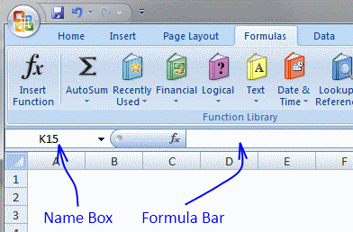
Copy cell B25 (Ctrl + c)
Select cell range B26:B10026 (Type B26:B10026 in name box and then press enter)
Paste (Ctrl + v)
Sarah,
AVERAGEIF(range, criteria, [average_range])
Finds average (average mean) for the cells specified by a given condition or criteria
AVERAGEIF function
Thank you so much Oscar you saved my day!
Hi Oscar, I was able to get the empty rows to show blank but I am still seeing some zeros on my worksheet. On my original spreadsheet with all the clients' info, there is a comment column that would be blank for some clients. When I put it on the new speadsheet with the lookup formula, those fields now shows a 0. Can you please shed some light on how to make them blank. Thanks again for your help.
Crystal,
Remove zeros
Hi Oscar,
Can you please show me how do I integrate the remove zeros formula into this formula:
=IFERROR(INDEX($C$3:$C$16, SMALL(IF($B$21=$B$3:$B$16, ROW($B$3:$B$16)-MIN(ROW($B$3:$B$16))+1, ""), ROW(A1))),"")
Thanks again!
Crystal,
Using your original formula I'm trying to figure out how to do wildcard matches. Can you help?
i.e. Search for CAR
Data
----
MART
CART
SCART
TRACK
CARRY
Results: CART, SCART, CARRY
EauMan,
Hey Oscar,
I have got this array formula working thanks to you, but I get these #NUM! error when all my values are extracted, because the formula is ongoing down the page, I want these #NUM! to display nothing, if there is no values left.
Help would be greatly appreciated !!
=INDEX(CBMSCHE,SMALL(IF(($N$2=$G$4:$G$60),ROW($G$4:$G$60)-MIN(ROW($G$4:$G$60))+1,""),ROW(A1)),2) +CTRL +SHIFT + ENTER.
Thanks.
Val,
Excel 2007:
Hey Oscar,
THANKS ALOT !!
It works perfect !! But I am trying it at home's laptop which has Excel 2007.
Do you know if it will work on Excel 2003 ???
THANK YOU !!
Hey Oscar,
I am trying the same formula at work, but in Excel 2003, and the #NAME? error now shows up. Do you know why it works differently in Excel 2003 & 2007 ??
& is there a possible solution on this?
Thanks again. !!
Hey Oscar,
Sorry for the repeated queries.
But I have figured it out.
Here is the formula that worked for me.
=IF(ROWS($A$1:A1)>SUMPRODUCT(--($N$2=$G$4:$G$60)), "", INDEX($H$4:$H$60, SMALL(IF($N$2=$G$4:$G$60, ROW($G$4:$G$60)-MIN(ROW($G$4:$G$60))+1, ""), ROW(A1)))) +CTRL +SHIFT + ENTER
thanks alot for your help !!
Hi oscar,
Please help me. What formula of vlookup i used to look up more value in another sheet if ever i enter id no.
Ex.Sheet 1
Id no Name Age
123 kia 30
234 ana 45
123 liza 65
879 meg 34
435 greg 13
I like this output in Sheet 2;
Id:______(if ever i choose 123)
output:Id no Name Age
123 kia 30
123 liza 65
thank you
anna,
read arnelias question
Thank you so much Oscar
Hi ocscar,
I try the formula you give to arnelia, but It does not work. Please help me. Please.. Send me a excel format please
thank you
anna,
Vlookup-return-multiple-records.xlsx
Hi Oscar,
Thank you so much....This is really great.
Tried using your formula on my project but am having some difficulties. First off had to change the "" to zero to get it to display a value, but now when it searches the price list it displays the first entry even though it doesn't match. It also won't display on the other cells when I copy and paste. If you can help in anyway I would greatly appreciate it.
=INDEX('Price List'!$A$3:$C$57000, SMALL(IF('Price Sheet'!$B$4='Price List'!$A$3:$A$57000, ROW('Price List'!$A$3:$A$57000)-MIN(ROW('Price List'!$A$3:$A$57000))+1, 0), ROW(A1)),COLUMN(A1))
BPV,
1, You can´t change "" to 0, then the formula returns the first record in your pricelist.
2, I am guessing here.. Maybe the value in 'Price Sheet'!$B$4 contains an additional space somewhere? Compare the values.
Hi oscar,
Thank you so much for help. But i notice the sample you send me, the database and output in one one sheet only, i try to separate the database and output using this formula:
=INDEX($A$2:$C$7, SMALL(IF($B$9=$A$2:$A$7, ROW($A$2:$A$7)-MIN(ROW($A$2:$A$7))+1, ""), ROW(A1)),COLUMN(A1)
But It does not work again. Please help me. Kindly send me again the excel sample that the output & database in separate sheet please please....Thank you
anna,
Get the Excel file
Vlookup - return multiple records.xlsx
(Excel 2007 Workbook *.xlsx)
1, You can´t change "" to 0, then the formula returns the first record in your pricelist.
2, I am guessing here.. Maybe the value in 'Price Sheet'!$B$4 contains an additional space somewhere? Compare the values
If I leave the "" in the formula I only returns a #VALUE!. I double checked and there is no additional spaces in the cell. Still not quite sure what the problem is.
Hi
This guide has gone directly to the top of my favorites. I've been loogin for this for so long!
But I still have a question.
I use this formula to put in all overdue invoices for my customers in a payment reminder letter.
So sometimes it is 1 invoice and sometimes it is 20 invoices or more.
Below the rows, where I am using your formula, I need to put in some plain text, but right now I has te be ind the very bottom of the page, and it doesn't look good when only one line is returned from the formula. Though it does look good when it is several rows.
Have you got any tips on how to make the area with formula flexible in how many rows it "occupies".
Hi Oscar....
THANK YOU SO MUCH.....
Hi,
is it possible to have the results in the same cell using a variation of your formula?..
I mean like:
John | x22 | John,Mark
John | x23 | John
John | x24 | John, George
Mark | x22 | John, Mark
George|x24 | John, George
The results separated by the comma in a single cell?...
And thanks a lot for your usefull code...
mcholst,
It is hard for me to give you advice without having seen your sheet.
anna,
you are welcome!
Ivan,
I believe this post describes what you are asking for: Excel udf: Lookup and return multiple values concatenated into one cell
VBA code:
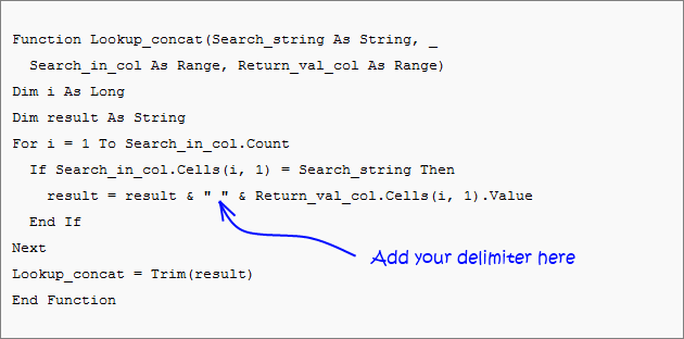
Hello,
thank you for your fast reply...
I'm not very good in excel and udf, anyway i followed your adivice, took your code and recreate a module.
The strange thing is that it gives me a blank cell (I took off the name of the sheet cause i want the results in the same one where the data are)..
Did i miss something?
Ivan,
Get the Excel file
Lookup and return multiple values concatenated into one cell.xls
(Excel 97-2003 Workbook *.xls)
Hello,
Does this only work with values in a single sheet? Is there a way to make this work across multiple sheets? I am using the macro and have this =IFERROR(Lookup_concat(G243,IndMtch!$A$2:$K$1773,IndMtch!$A$2:$A$1773),"NA") and it is returning NA even though there are values that match in the areas specified. I am using Excel 2007.
Thank you for your assistance in advance!
thank you a lot..
It works perfectly
Oscar,
I've been searching all over (to no avail) for a lead on how to return multiple values from one sheet onto a summary sheet but the tough part is that the criteria for the is that the date be "=>"&today(). I want to return any dates from one sheet onto the summary sheet IF those dates equal today or a future date, but not a past date. Any thoughts?
Thanks.
Oscar, I'm looking for something like this page on your site: https://www.get-digital-help.com/excel-find-latest-date-in-a-list/ except that I'd like it to return the last ten values, provided those fit the date criteria of >=today. I'd like to do that on a different sheet than the sheet where the original values are, because I will have multiple sheets that I will need to similarly pull the values from onto the summary sheet.
Renee,
I believe this post answers your question:
List names whos date has past in excel
Array formula:
Create named ranges or replace with absolute cell references.
How to create an array formula
1.Copy (Ctrl + c) and paste (Ctrl + v) array formula into formula bar.
2.Press and hold Ctrl + Shift.
3.Press Enter once.
4.Release all keys.
Excellent! This worked like a charm and I was able to use it with a Sheet! reference.
One more question, how do I get rid of the #NUM! errors that show up in the column that doesn't have a value to return (yet)?
Thanks so much.
I got it! Thank you SO much for your help. I have spent hours trying to figure this out.
Renee,
I am happy you figured it out.
Here is how to remove #num errors, for those of you who wants to know.
=IFERROR(formula, "")
Ok, in excel I want to lookup the value of column B where the value in column F equals "1" exactly. I then want to add up the value in B for each match until the table column F8:F202 has been checked for matches :
For example
Col B ----- Col F
10 ----- 1
1 ----- 1
0 ----- 0
1 ----- 10
2 ----- 1
I would expect the formula to return 13, due to "10 x 1", "1 x 1" and "2 x 1" matching = 10 + 1 + 2 = 13
To me, the formula should contain a LOOKUP and SUMIF statement.
I've tried several formulaes, but without joy. Your help would be appreciated.
Sean,
Hi oscar,
It possible can use vlookup only and will not use the index to get the output on this:
Sheet1
id name status
123 ANNA active
124 jhun separated
125 liza active
129 roy separated
789 mary separated
123 anna separated
Sheet2:
Enter id:123
123 ANNA active
123 anna separated
Hi Oscar,
Do you know whats wrong in my formula?
=INDEX(deletion,SMALL(IF($A$7=DELETION!$B$3:$B$500,ROW(DELETION!$B$3:$B$500)-MIN(ROW(DELETION!$B$3:$B$500))+1,""),ROW(B11)),COLUMN(B11)
Thank you.....
ANA,
Question 1
Sorry, I don´t know how.
Question 2
=INDEX(deletion,SMALL(IF($A$7=DELETION!$B$3:$B$500,ROW(DELETION!$B$3:$B$500)-MIN(ROW(DELETION!$B$3:$B$500))+1,""),ROW(A1),COLUMN(A1))
The cell references in column and row functions always start with A1.
hi Oscar
Thank you so much for your help. One question again if ever my output like this and i would like to hide #num. What formula i can used?
Enter id:123
123 ANNA active
123 anna separated
#num #num #num
Here's my use formula.
=INDEX(deletion,SMALL(IF($A$7=DELETION!$B$1:$B$499,ROW(DELETION!$B$1:$B$499)-MIN(ROW(DELETION!$B$1:$B$499))+1,""),ROW(B1)),COLUMN(B1))
Thank you in advance
ANA,
Excel 2007:
Excel 2003:
Hi Oscar,
THANK YOU SO MUCH.......
Oscar,
Only just got an email saying there is a reply.
Tried the formulae out and it worked a treat.
Is there a particular book on excel that would be an ideal guide on some of the questions you are asked, or is it a case of trial and error ?
Very much appreciated.
Séan
Oscar,
Now for another puzzle. I have a datasheet which I produce several pivot tables on worksheets within the excel document. One column is a hyperlink to an internal website :
https://companyweb/Lists/Sales%20Product%20Information/DispForm.aspx?ID=1
This is kept on a worksheet called "Pivot Data". To update this data, I cut and paste the values over the top of the current data, so on effect, the number of rows will vary.
Is there a way of making this cell automatically recognises the hyperlink and updates accordingly ?
When you refresh the data, so that each of the pivot tables are updated with the new data, is it then possible to make sure that the data of the hyperlink is shown as a valid hyperlink which can be pressed with left mouse button on and redirected., i.e. The worksheet "Customer Sales" is a pivot table based on the "Pivot Data" worksheet and the column title for the hyperlink data is "Notes".
I know I'm asking a bit much, but I'm sure there is a solution and at the moment I'm struggling to find one.
Regards
Séan
Hi Oscar,
First time here so please bear with me. I've searched just about everywhere for a formula that can help me. I'm using the
=INDEX($A$2:$C$7, SMALL(IF($B$9=$A$2:$A$7, ROW($A$2:$A$7)-MIN(ROW($A$2:$A$7))+1, ""), ROW(A1)),COLUMN(A1))
formula to return multiple records. I have tried to modify it but to no avail. Where your formula matches the cell in $B$9 exactly, I would want to simply put part of the value in $B$9 and let the formula return all that match it e.g. you use 123 and it shows you all the 123 and adjacent values but I would want to enter e.g. only 12 and would want it to return all values that contain 12.
The above is basically to be used to look for product codes. I have an array of 4 columns with product codes in 1st column and need e.g. all products starting with "CP-" and also displaying all adjacent values that come with the particular product code. Not sure if I'm being clear enough.
example:
product code...column2...column3...column4
MB-DKJ3475.....1122......N.........product description
CH-UYI2938.....125.......N.........product description
CP-DLK4378.....4258......C.........product description
CC-DDD3429.....26553.....C.........product description
CP-LKL4344.....33........C.........product description
I would want all the product lines starting with "CP-":
CP-DLK4378.....4258......C.........product description
CP-LKL4344.....33........C.........product description
Greatfull for any help that you might be able to provide.
Many thanks in advance
Regards
Coenraad
Sean,
Is there a particular book on excel that would be an ideal guide on some of the questions you are asked, or is it a case of trial and error ?
As far as I know, there is not much written about array formulas.
I got interested in array formulas when I discovered Dennis Wallentin website: https://xldennis.se/ . It is in swedish.
I am inspired by comments on my website, other forums and excel sites.
There is also a lot of trial and error.
Sean,
Now for another puzzle. I have a datasheet which I produce several pivot tables on worksheets within the excel document. One column is a hyperlink to an internal website :
https://companyweb/Lists/Sales%20Product%20Information/DispForm.aspx?ID=1
This is kept on a worksheet called "Pivot Data". To update this data, I cut and paste the values over the top of the current data, so on effect, the number of rows will vary.
Is there a way of making this cell automatically recognises the hyperlink and updates accordingly ?
Yes, import data from the web using web queries.
Here are some resources:
https://office.microsoft.com/en-us/excel-help/get-and-analyze-data-from-the-web-in-excel-HA001054848.aspx
https://www.openjason.com/2008/01/25/3-steps-to-scrape-the-web-with-microsoft-excel/
https://www.vertex42.com/News/excel-web-query.html
How to recognize url in sheet1 cell A1
Function Identifyaddress() As Boolean
    If Sheets("Sheet1").Range("A1").Value = "https://companyweb/Lists/Sales%20Product%20Information/DispForm.aspx?ID=1" Then
        Identifyaddress = True
    Else
        Identifyaddress = False
    End If
End Function
When you refresh the data, so that each of the pivot tables are updated with the new data,
Sure, use tables. They are dynamic. You need vba to refresh pivot tables automatically: Auto refresh a pivot table in excel
is it then possible to make sure that the data of the hyperlink is shown as a valid hyperlink which can be pressed on and redirected.,
You need a macro to accomplish this.
i.e. The worksheet "Customer Sales" is a pivot table based on the "Pivot Data" worksheet and the column title for the hyperlink data is "Notes".
Coenraad,
I believe you are looking for this post:
Lookup with multiple criteria and display multiple search results using excel formula
Array formula in cell A10
Cell $A$8 contains the search value.
How to create an array formula
Copy (Ctrl + c) and paste (Ctrl + v) array formula into formula bar.
Press and hold Ctrl + Shift.
Press Enter once.
Release all keys.
How to copy array formula
Select cell A10
Copy (Ctrl + c)
Select cell range A10:D12
Paste (Ctrl + v)
Oscar,
I'll look into. Thanks again.
What if the ID changes, and may not be the same in each cell ?
https://companyweb/Lists/Sales%20Product%20Information/DispForm.aspx?ID=1
or
https://companyweb/Lists/Sales%20Product%20Information/DispForm.aspx?ID=2
or
https://companyweb/Lists/Sales%20Product%20Information/DispForm.aspx?ID=....
Oscar,
Thanks a mil for that. Works perfectly. You saved me a major headache.
Thanks again and have a great day.
Oscar,
I think I have probably confused the issue. The data is on a worksheet within the document containing the pivot tables on other worksheets.
None of the data comes from the web, just that one column of the data may include the hyperlink provided ( "?ID=x" where x is a varaible ).
Basically, when I do a refresh of the data in the "pivotdata" worksheet, I need it to recognise the cell is a hyperlink. In addition, when I update the indivital pivot tables, it looks at the data in the "Notes" field and recognise it as a hyperlink.
Where do I put the "Function Identifyaddress()" information you gave.
Regards
Sean
Hi Oscar,
First, this formula is genius. And now that I buttered you up, here's my question. I wanted to use this but to have the data on another worksheet. So I:
=INDEX(Masterdata, SMALL(IF($B$2=colrow, ROW(colrow)-MIN(ROW(colrow))+1, ""), ROW(Master!B2)),COLUMN(Master!B2))
This works until I drag the formula down to include additional results and Master!B2 becomes Master!B3. At that point, I get a Number error.
I guess I would like to know why the number error occurs, but more importantly, if there is an error free way to use this formula to return data on another worksheet.
Thanks a mil.
KJ
Sean,
I am confused, it is difficult for me to understand without the workbook.
KJ,
The number error occurs because there are no matching cells left in formula.
Your formula must start with cell reference A1. Bolded in formula below.
Example,
Excel 2007, remove #num errors:
Oscar,
Thanks so much. Worked like a charm.
I have a large database with 40 columns, I wish to extract a few column data into separate sheet for printing. The goal is actually a male name list and a female name list with another criteria from a column that is confirmed. Which page shows the examples?
Thank you
Alex Chiok
Hi, Thanks for valuable home page,
I want formula to find 2 valuse for the same ID, if I have long list with over 1000 ID's and want to find Anna and the status if she is active or not. How I should write my formula.
Thanks and have a great day.
Alex Chiok,
Excel tables are easy and fast!
https://office.microsoft.com/en-us/excel-help/overview-of-excel-tables-HA010048546.aspx
Oscar,
Did you receive the workbook I emailed you ? If so, any joy with finding a solution to my problem ?
Sean,
Basically, when I do a refresh of the data in the "pivotdata" worksheet, I need it to recognise the cell is a hyperlink. In addition, when I update the indivital pivot tables, it looks at the data in the "Notes" field and recognise it as a hyperlink.
I am still confused. You want the data in column "Notes" being recognized as a hyperlink in a pivot table? So you can press with left mouse button on an hyperlink a pivot table and it automatically opens a webpage in a webbrowser?
Correct on both counts. Does this sound feasible ?
Your help is very much appreciated.
Regards
Sean
Sean,
USING HYPERLINKS
Unlike external data ranges, active hyperlinks are not supported in PivotTable cells. The hyperlink is treated as text, but you cannot follow the hyperlink to a Web page or document, in Excel or Excel Services.
Source: Use a PivotTable report to make external table data available in Excel Services
Oh well :-( thanks for trying.
Kind Regards
Sean
thanks,
it really work for me...
now, i can make my accounting book more light
Hi I am using your formula where the data is in another tab but it does not seem to work for me.
=INDEX(Activities,SMALL(IF($B$3=NameID, ROW(NameID)-MIN(ROW(NameID))+1, ""), ROW(Data!C2)),COLUMN(Data!C2))
Activites = Data!C2:G27
NameID = Data!C2:C27
I am trying to return the same way as your example INDEX($A$2:$C$7, SMALL(IF($B$9=$A$2:$A$7, ROW($A$2:$A$7)-MIN(ROW($A$2:$A$7))+1, ""), ROW(A1)),COLUMN(A1))
Can you let me know what I am doign wrong?
Thanks
This is great. Thanks a lot for posting this. You've saved me a bunch of time.
Is it possible to use this to grab data from multiple sheets at once? I see how KJ has pointed it at a single different sheet, above, but my data is spread over 31 sheets all using the same template.
Thanks again.
I did not read the KJ post above. I changed to A1 and it worked just fine. Thanks again for showing the formula
Please forgive my limited knowledge, but is an "add-in" the same as a "module"? This seems like the solution I might need to purchase and put into play, but all of my data is on a single worksheet and performance is significantly slowing. I believe that performance could be improved by an add-in or module that could be "accessed" through a message box? Thanks for any advice or assistance!! The distension of the vein in my forehead means that I've just reached certain limits in trying to solve these issues on my own!
Jim,
No, you don´t need to buy this addin.
I will soon add a custom function to this blog post: How to return multiple values using vlookup in excel
Sean,
See this post: Follow hyperlinks in a pivot table
Andrew,
No, I have no idea how to accomplish that with array formulas.
Jim,
I have now added a custom function!
https://www.get-digital-help.com/how-to-return-multiple-values-using-vlookup-in-excel/#vba
Hi Oscar.
Your posts are really helpful and informative - and much appreciated. I have, however, got totally stuck with my example.
I have the following lookup values:
pen
eraser
paper
paper clip
and the following item list:
Allan's pen
eraser
Frances' eraser
Jenny's pen
paper
paper clip
pen
red pen
What I’d like to do is search for each lookup value in the item list and return all the items that contain that text string. For example, 'pen' would return (in adjacent cells):
Allan’s pen Jenny’s pen pen red pen
I have spent several days trying to tweak your examples, to no avail. Can you help or point me in the right direction, please? Many thanks.
Oscar,
I lifted your example verbatium and updated it for my 83 records. The if statement hangs on #value!. I moved it from below the data (row)and placed it in the first available column. The if statement works, but only on the respective row. Thus will not pick up the mutliple's?
Where'd I go wrong?
Thank you
You have got one hell of a great method of doing this. I had a found a similar solution some time ago, but that used a VBA custom formula to return arrays. This is better because there is no VBA. Thank you.
However, one big problem: Arrays take a very long time in calculating. I do not know why, but I had to find a solution. Turns out that making each cell an array is the wrong way of doing things.
I will give you my example:
I have a log of material receipts;
I have several sheets in excel that retrieves a list of receipts corresponding to a certain type;
The log has details of each receipt, e.g. date, reciept #, store, delivery type, qty, cost.
If I have say 60 types of materials and at least 30 rows on each sheet with 6 columns, I will have 10800 arrays. That is about 30 seconds of calculation. Far too many for practicality. So I made one array per sheet and I modified the formula so that the last two functions (row and col) have arrays as arguments. Much simpler then. But requires a little more explanation.
Thanks.
If I was not clear enough: Each sheet fetches receipts of a certain type from the log.
I have been working on a worksheet and cannot figure out the formula that would work to copy to the other cells and result in the duplicate entries being shown. I want to enter the phone number in the phone column and have the last name and address populate. Can you give me some guidance? Thanks.
A B C E F G H
1 2 3 4
Phone Last Address 330-555-9235 Adams Mary 12 Oak St.
330-555-8099 Adams Michael 44 Oak St.
330-555-8119 Adams Sam 44 Oak St.
330-555-5566 Jones Mary 36 Main St.
330-555-5327 Palmer Michael 67 ShortSt.
330-555-2227 Powers Sara 27 ShortSt.
330-555-7845 Parker Clarence12 Oak St.
330-555-6565 Parker Mary 36 Main St.
330-555-7901 Smith Clarenc 513 Main St
330-555-7901 Miller Sam 517 E. Main
Help,
Completely perplexed. I can't alter the formula at all without getting the #value! error. What's wrong? I can insert into your example "tbl" but no alteration or edit or open or the formula without the #value!. Any suggestions would be nice?
RE,
Oscar,
I lifted your example verbatium and updated it for my 83 records. The if statement hangs on #value!. I moved it from below the data (row)and placed it in the first available column. The if statement works, but only on the respective row. Thus will not pick up the mutliple's?
Where'd I go wrong?
Thank you
Completely perplexed. I can't alter the formula at all without getting the #value! error. What's wrong? I can insert into your example "tbl" but no alteration or edit or open or the formula without the #value!. Any suggestions would be nice?
Suggestions:
Did you change cell references in the formula? Cell references are bolded:
The first formula must start with cell reference A1 (bolded), example:
Did you create an array formula?
Anas Hashmi,
Yes, you are right. Array formulas are too slow with large data sets.
Stephanie,
Can you explain this in greater detail?
I have been working on a worksheet and cannot figure out the formula that would work to copy to the other cells and result in the duplicate entries being shown.
Ok,ok...The Control, Shift, Enter thing I completely missed. After editing the formula you must re-enter formula via this key combination. As expected the formula is genius... 4 days later!
So thank you and can you now point me in the right direction. I have a column of cities (multiple), each city row has a color, red, green, blue, etc.. associated with it. The row and column formula works, but grows my data base in rows. I have my colors in columns and want to populate the color column as it applies to the city on a single row basis. The column formula works well, but I can't be assured that all colors will show up in their respective columns with in the city row.
Thus red green, blue, its possible that if green is not in the data, blue data falls into the green column.
Suggestions?
Any advise how to sort on city, and populate columns that apply to specific colors?
RE,
I am not sure I understand.
Get the Excel file
re-city-color.xlsx
From my comma delimited file dump:
Office# City Color Code ID
OF175 Ames Blue 672
OF175 Ames Red 8732
OF25 Oakmont Green 753
OF25 Oakmont Blue 8743
OF5 Omaha Red 634
OF95 Dallas Red 231
OF95 Dallas Blue 13244
OF95 Dallas Orange 13132
OF95 Dallas Pink 234
My Spreadsheet desired result
Office# City State Red Green Blue Orange
OF175 Ames Ia 8732 672
OF25 Oakmont Mn 753 8743
OF5 Omaha Ne 634
OF95 Dallas Tx 231 13244 13132
I'm trying to get from comma delimited rows to a consolidated row where the color code lines up and populates the cell with the ID.
Thank you for your time
Does this help?
Sorry it lost the formatting when I sent it,
CSV: Office# | City | Color |ID |
Excel: Office# | City | State | Red | Green | Blue | Orange
Stephanie,
read this post: https://www.get-digital-help.com/excel-array-formula-enter-a-value-in-a-cell-and-instantly-populate-adjacent-cells/
Oscar,
I guess it can't be done? Eh?
Re,
I am sorry, I somehow missed your comment.
Check out this file: re-city-color1.xlsx
Hi, Oscar...
I have been looking for help on "How to return multiple values using vlookup in excel" for one whole day... then I found this... Man!, you help me so much. Thanks for sharing your knowledge. God Bless
Erwin,
Thanks!
Hello,
Thanks for the helpful formula. I used this formula successfully, but now I wanted to get the data I missed with the formula. How would you add multiple IF/AND statements to the formula. For example add:
(IF($B$8<$B$2:$B$6,...),($C$8<$C$2:$C$6,...), etc.
Thanks!
Kevin,
I used this formula successfully, but now I wanted to get the data I missed with the formula.
What are you trying to do?
How would you add multiple IF/AND statements to the formula. For example add:
(IF($B$8<$B$2:$B$6,...),($C$8<$C$2:$C$6,...), etc.
Oscar, great post. One question: I am using the vba code you provided and it works great. I am dealing with a set of 110,000+ rows of data (2 columns) with about 17,500 unique lookup values and the remainder of the rows are unique values to be found. I need to use the vba that you posted but to have it output the data horizontally, not a vertical array. I am terrible with VBA. Any chance you could give me some pointers or tell me which part of the code to change. Any help would be much appreciated.
Ex:
35007000030002 354CSTRL
35007000030002 354CSTRU
35007000030002 402MRRW
35007000030003 404CHRK
35007000040000 402MRRW
Needs to become:
35007000030002 354CSTRL 354CSTRU 402MRRW
35007000030003 404CHRK
35007000040000 402MRRW
When looked up.
Sorry, my question was vague. Here is the setup of my worksheet:
I have 3 columns filled with percentages associated with W,X,Y,Z.
% red %pink % blue
10% 15% 30% W
25% 33% 80% X
40% 12% 66% Y
75% 4% 12% Z
I used your formula to find W,X,Y,Z meeting the below criteria:
>30% red >20% pink >50% blue
Y X X
Z Y
Now, I want to find one formula that will find the values not captured by the previous formulas. In other words, (% red <30%)(% pink <20%)( % blue <50%) = W
Thanks!
Jonathan ,
I have changed the existing udf on this webpage. It is now possible to return values horizontally.
Kevin,
Get the Excel file:
Vlookup-kevin.xls
Oscar, great job! keeping the thread alive for so long! This is a great one!
I have a question around merged cells. Lets say in your first example, Both Pen and Paper cost $5, so I have merged C2 and C3 into a single cell with the $5.
Now, in the search cell (B8), if I put in Pen, it will give me the correct asnwer. However, if I put in Paper it will not return the value, as opposed to the expected returned value of $5.
The question: is there a way to make this work with merged cells
Greatly appreciate you help.
Hass
Hass,
There is question I don´t know the answer to!
I would avoid merged cells as much as possible.
Hi Oscar,
The VLOOKUP "Return multiple values horizontally" is exactly what I need, however it is not working for me. I copied everything exactly as shown in your example, but all I get is "#VALUE!". I am using Excel 2010 on a PC. Has something changed in the 2010 version, or am I just missing something?
would it be possible for the formula to copy itself into other cells below depending on how amny unique references were found in the table?
Kieran,
That would require vba.
Janet,
Maybe you forgot to create an array formula? Instructions are in the post above.
Hi Oscar,
The array formula I used was the same as in your "Return Multiple Values Horizontally" example: "=INDEX($C$2:$C$6, SMALL(IF($B$9=$B$2:$B$6, ROW($B$2:$B$6)-MIN(ROW($B$2:$B$6))+1, ""), COLUMN(A1)))". I set up the table exactly as you show in your example as well, but it isn't working for me. All I get in cell C9 is #VALUE! Any ideas on why it isn't working?
Thanks.
I have multiple worksheets in an excel book. I have a drop down menu on the worksheet entitles "ON Work" The drop down menu is in cell B50
I then need to be able to look up whatever option is picked in B50 and look up mulitple values from a different worksheet entiled "Panels" the Panels table goes from A1:F80
So if i choose the option 140XL in B50 below it I need all the information from the "panels" sheet that corresponds with 140XL.
The Panels Sheet information is set up like this:
140XL 12025 16" Large
140XL 58625 12" Small
140XL 99951 12" Rear
So i need it to look up 140XL and get the infromation 12025,58625,9951
i have looked all over the interent for help and it's either way too confusing or doesn't deal with multiple worksheets. I know it is possible but i really am our of ideas
Janet,
Get the Excel example file:
Return-multiple-values-horizontally.xls
I am trying to use the formula for a bigger range, C3:C40. I modified the formula as follows -
=INDEX('Resource Project Mapping'!C3:C40,SMALL(IF($B$4='Resource Project Mapping'!B3:B40,ROW('Resource Project Mapping'!B3:B40)-MIN(ROW('Resource Project Mapping'!B3:B40))+1,""),ROW('Resource Project Mapping'!A1)))
however I am getting the below results
#VALUE!
#NUM!
#NUM!
#NUM!
#NUM!
Can you please help?
DP,
You need to use absolute cell references (except the last cell reference):
DP,
You can find my answer here: How to return multiple values using vlookup
hi,
I have multiple worksheets in an excel book. I have a drop down menu on the worksheet entitles "ON Work" The drop down menu is in cell B50
I then need to be able to look up whatever option is picked in B50 and look up mulitple values from a different worksheet entiled "Panels" the Panels table goes from A1:F80
So if i choose the option 140XL in B50 below it I need all the information from the "panels" sheet that corresponds with 140XL.
The Panels Sheet information is set up like this:
140XL 12025 16" Large
140XL 58625 12" Small
140XL 99951 12" Rear
So i need it to look up 140XL and get the infromation 12025,58625,9951
i have looked all over the interent for help and it's either way too confusing or doesn't deal with multiple worksheets. I know it is possible but i really am our of ideas
Please Help!
Ainslie,
read this post:
Use a drop down list to search and return multiple values
Dear,
I want to copy the formula from first cell to its adjacent cells, but I want to keep the same value of the last cell to be multiplied with the above percentage, but when I paste the formula into adjacent cell it copies the value of the cell next to the one I need the value from
please advise
Hi Oscar,
I'm trying to use your vbaVlookup tool, and am having issues where by lookup columns are backwards from yours (switch the price and pen columns around), and I want to find all of the matches from the first column, not the second one. When I use the formula, it just returns a blank. It works fine if I switch the columns, but this is not ideal.
Here's an example:
A B
AAA GrpA
BBB GrpA
CCC GrpB
DDD GrpA
EEE GrpC
I then create another column elsewhere, with "GrpA" as a header, then in the second row of that column, my function looks like this:
{=vbaVlookup(C1,$A$2:$B$15,1)}
I figured the last parameter (1) was to look at the first column instead of the second.
If you could provide some help to get this working, that would be superb. Thanks!
Feras,
Can you describe in greater detail and some example values?
Ben,
get the file:
Ben.xls
Oscar,
Is it possible to return the values in the next tab or sheet? instead of the same sheet?
Oscar, Pls ignore above.
I got how to do :)
Hi Oscar,
Thanks for this article... the formula has been a great help to me in setting up some of my worksheets. I have a question about it though:
=INDEX($A$2:$C$7, SMALL(IF($B$9=$A$2:$A$7, ROW($A$2:$A$7)-MIN(ROW($A$2:$A$7))+1, ""), ROW(A1))
Is it necessary to use the "MIN(ROW(array))+1" calculation? I was looking at a similar formula posted by Ashish Mathur and I noticed he didn't use the "MIN...".
Thanks
Timus,
You can also use MATCH(ROW($A$2:$A$7), ROW($A$2:$A$7)).
becomes
In fact, you can use: ROW($1:$7)
and the formula becomes:
Remember, if you then replace your cell references with named ranges, the last formula won´t work. It is not dynamic contrary to the other two formulas.
Thanks for commenting!
Hi Oscar,
It's really amazing!!! And you explain it so well!
I have searched for it so much.
Thanks a lot!!!!!
But still I have a question:
I would like that if there is nothing more to find, the formula will return a blank cell and not "#NUM!".
Is it possible?!
Hi Oscar, Thank you for your posting. My question is fairly basic. I recreated your table of "Return multiple values vertically" above and entered the exact formula. However, it doesn't work.
I entered in the C8 cell --> =INDEX($C$2:$C$6, SMALL(IF($B$8=$B$2:$B$6,ROW($B$2:$B$6)-MIN(ROW($B$2:$B$6))+1),ROW(A1)))
And excel gave me -- > #VALUE!
If I copied your formula directly from the formula bar to my sheet in C8 cell, excel would return #VALUE! as well. However, if I copied an entire cell, and paste into my C8, excel would return exact same value as your original table. I am using Excel Mac 2008 but I don't believe this would have anything to do with it. Please let me know. I really appreciate your time. Thank you very much.
Just want to tell you: THANK YOU! Your web is great, your are very generous. Thank you for sharing!
Noa,
Excel 2007
Dawisee,
You forgot to create an array formula.
How to create an array formula
1. Press with left mouse button twice on cell C8.
2. Paste formula
3. Press and hold Ctrl + Shift
4. Press Enter
Gab,
Thank you for commenting!
My formula no working, I follow your steps but there´s somethink wrong..., please give me a hand!
=INDEX($B$1:$C$700;SMALL(IF(($D$90=$B$1:$B$700);ROW($B$1:$B$700)-MIN(ROW($B$1:$B$700))+1;"");ROW(A1));2)
VIC,
I think you forgot to create an array formula.
=LEFT(INDEX($C$2:$C$13546,SMALL(IF($E$3=$B$2:$B$1300,ROW($B$2:$B$1300)-MIN(ROW($B$2:$B$1300))+1,""),COLUMN(A1))),11)
Hi Oscar,
Your code works perfect but hen I reach $B$1300 or more the result will be #VALUE! Please help!
thanks a lot,
jener
Oscar,
I am trying to do a vlookup between multiple worksheets but there are a few duplicates with the same value. Do I need to purchase the addin if I want it to pull back the duplicates?
Jener,
adjust cell references (bolded):
Penny,
You can use the example in this post if you have 2 sheets. It will also get duplicate values.
The addin returns all values, unique distinct values and duplicate values from two or more sheets. Press with left mouse button on the examples above.
You can use this contact form if you have more questions.
Hi Oscar,
thanks for the reply,
I have no clue how to adjust it.
Can you give me a sample. lets say in Column B and C there are 100000 rows
Is this the right code for it:
=LEFT(INDEX($C$2:$C$100000,SMALL(IF($E$3=$B$2:$B$100000,ROW($B$2:$B$100000)-MIN(ROW($B$2:$B$100000))+1,""),COLUMN(A1))),11)
need your expert advice,
jener
Jener,
I thought you copied the array formula horizontally? You are using column(A1) in your formula.
Your example seems to be right.
Oscar,
I am using this formula and have found that it does not produce all of the results from the data file.
My data sheet contains:
Column (A) - Account Number
Column (B) - Date
Column (C) - Notes
There are 1 - 15 instances of the account number in Column (A).
The instances may be on different or the same day (date) in column (B).
The notes in Column (C) are all different.
The results being returned are limited to only two rows per date.
So if I have 5 Notes on 01/01/2012....the results are only returning 2 of them...it appears to be the two middle rows.
Can you help.
Thanks for the great formula!!
I should have included the formula mentioned above just to be clear:
=INDEX(COMMENTS!$I$2:$I$15000, SMALL(IF((GET_COMMENTS!$E$3=COMMENTS!$A$2:$A$15000)*(GET_COMMENTS!$E$3=COMMENTS!$A$2:$A$15000), ROW(COMMENTS!$A$2:$A$15000)-MIN(ROW(COMMENTS!$A$2:$A$15000))+1, ""), ROW(A1)))
Oscar,
Nevermind, I'm loosing it. Too many hours in front of a spreadsheet. :)
beth,
Get the Excel file:
beth.xlsx
Hi Oscar,
Im using the "Return multiple values vertically or horizontally (vba)". Right know I can get it to return 3 values in the the cells C9-C11. I have a lot of data to lookup and would like it to return more values vertically (maybe 10 values). When I try to copy the array to the next cells, I either get a error message og it will start returning the same values, is already shown in C9-C11. Can you help me? (Hope the question makes sense)
Ulrik
Hi Oscar,
First of all, thank you VERY much for the superb effort you put in for us Excel newbies to be better!
I am facing one problem in making this array formula run. My data table and output table are on different sheets. While the formula works perfectly when they are both in the same sheet, error is returned when they are on different sheets. Here's my formula that works:
=IFERROR(INDEX($A$2:$E$107, SMALL(IF(Dashboard!$C$6=$A$2:$E$107, ROW($A$2:$A$107)-MIN(ROW($A$2:$A$107))+1, ""), ROW(A1)),COLUMN(A1)),"No More Data Available")
Here's the one that does NOT work:
=IFERROR(INDEX('Business Events'!$B$2:$E$3177, SMALL(IF($C$6='Business Events'!$B$2:$E$3177, ROW('Business Events'!$B$2:$B$3177)-MIN(ROW('Business Events'!$B$2:$B$3177))+1, ""), ROW('Business Events'!B1)),COLUMN('Business Events'!B1)),"No More Data Available")
Data table is in sheet named "Business Events" and output table is in another sheet named "Dashboard". The filtering id is in cell C6 in the sheet "Dashboard".
Please help.
Thanks much!
Soumit
Soumit,
Does this formula work?
Ulrik,
I think the problem is how you enter the udf.
You can´t copy an array formula returning two or more values.
How to expand the array formula from cell range C9:C11 to C9:C21
1. Select C9:C21
2. Press with left mouse button in formula bar
3. Press and hold Ctrl + Shift
4. Press Enter
5. Release all keys.
Thanks for bringing this to my attention.
Hi Oscar,
Thanks much for your guide, it is helping out tremendously. I am wanting to alter your code a bit, and it seems like it should work but I am not getting the desired results. I would like to have an if or to check for another value. This is how I assumed it would look, but again, I'm not seeing the desired results. Assume C9 had 124.
=INDEX($A$2:$C$7, SMALL(IF(OR($B$9=$A$2:$A$7, $C$9=$A$2:$A$7), ROW($A$2:$A$7)-MIN(ROW($A$2:$A$7))+1, ""), ROW(A1)),COLUMN(A1))
I would like results for 123 and 124. I however seem to be getting every thing back as a result. What is going wrong? Thanks much for your help!
Mat,
($B$9=$A$2:$A$7)+($C$9=$A$2:$A$7) returns an array
OR($B$9=$A$2:$A$7,$C$9=$A$2:$A$7) returns a single value.
Beautiful! Thank you very much!
Hi Oscar,
Did you post a thread regarding INDEX/MATCH with Multiples criteria?
mean to say, one index range and one match range , but with two or more values to consider to return equivalent index?
ex: column A with various brands (index) and column B with corresponding types of car (sedan, coupe, suv, van...).
query in column C asking for brands having sedan & coupe or sedan & coupe & suv would return corresponding brands.
Thanks to advise thread where is was posted.
Oscar,
sorry, I got it:
IFERROR(INDEX(INDEX RANGE,SMALL(IF(ISNUMBER(MATCH($MATCH RANGE,CRITERIA RANGE,0)),ROW(INDEX RANGE)-ROW($C$2)+1),ROWS(LOCATION OF QUERY))),"")
{IFERROR(INDEX($A$2:$A$10,SMALL(IF(ISNUMBER(MATCH($C$2:$C$10,$I$1:$I$2,0)),ROW($A$2:$A$10)-ROW($C$2)+1),ROWS($I$3:I3))),"")}
I changed location of match to column C and formula is in column I just under the two (2) criteria.
However... i still get redondant feedback from index range... have a look if you can:
https://uploading.com/files/m4613588/oscar.xlsx/
Thank you Oscar, worked perfectly.
Cyril,
I think this is the post you are looking for:
Vlookup with 2 or more lookup criteria and return multiple matches in excel
Oscar, my apologies! The formula works exactly as (not) advertised, I screwed up on the accuracy of the id value. Basically the id matched no value on the data table, as a result the obvious error was displayed. Next time, I will make sure I am more diligent at my end before posting.
Anyway, thanks to you, I learned a great way to "query" an excel "Database" :)
Best regards-
Soumit
Hello,
I used the formula to get multiple values, and works great. My look-up values are available in the "Data" sheet. The result of look-up is in the "Summary" sheet. There is a percentage calculation in 'summary' sheet which is simple calculation like =g5/g7, and I want to sort values in descending order based on percentages. When I sorted results in the "summary" sheet, the sort was not applied. I guess it is because of "Index" formula. Frankly, I am lost as to how to apply sort. Could you please advise what should I do? Thanks for your help.
Best regards,
Prashant
Oscar,
Thanks for the reply, however I end up with the same situation as with my formula (posted on feb 13.
In the file I uploaded, have a look at column I, I placed a note for you there with a specific example.
I still get redundant (double) entries from the index... i'll try to add a condition to the formula, please have a look when you can spare some time, you might have (definitely) a better solution.
Cheers,
Cyril.
Oscar,
Thanks for your answer!!
Thanks for this formuls
This is working nice
but i need some different than because in my data is with ,
like below
please help me if there is any formula to find from this kind of data
700-AT-003,700-AT-004,700-AT-005,700-AT-006 IAN010061113
700-AT-005 IAN020000001
700-AT-005 IAN020000004
700-AT-004 IAN020000013
700-AT-003 IAN020000015
700-AT-003, IAN020000017
700-AT-006 IAN000036102
700-AT-005 IAN000036103
700-AT-006 IAN000041102
700-AT-003,700-AT-004,700-AT-005,700-AT-006 IAN020000010
700-AT-004 IAN010061104
thanks
Oscar,
Allow me to say thanks for sharing this info.
lucky that I found this & save me a lot of effort.
I took over 2 hrs to understand the original one,
at the I finally understand the whole logic & able to modified the formula to suit my purpose.
this is my latest version of the formula based on your original sharing:
-------------------------------------------------------------------
=IF(ISERROR(INDEX(PMO_Prj,SMALL(IF(($C$1=Project_Status),ROW(Project_Status),""),ROW($A1)),COLUMN(Date_Esculate_to_MDM))),"",IF(INDEX(PMO_Prj,SMALL(IF(($C$1=Project_Status),ROW(Project_Status),""),ROW($A1)),COLUMN(Date_Esculate_to_MDM))=0,"",INDEX(PMO_Prj,SMALL(IF(($C$1=Project_Status),ROW(Project_Status),""),ROW($A1)),COLUMN(Date_Esculate_to_MDM))))
-------------------------------------------------------------------
with some of the column associate with Name (in this case, "Date_Esculate_to_MDM" )
of which this would allow the cell to refresh with accord to the user select in cell [C1], plus show blank when cell either contain nothing or caused error.
allow me to say thanks again for sharing this.
Oscar,
thank you very much! It helped a lot to solve my problems!
Hi Oscar,
I have a problem with lookups in different sheet. In first sheet, in first column I have names of people. In second column i have dates. There are more sheets in the workbook named by dates containing names of people and amounts. Now in third column i have to get amounts by looking up the names from first column in the specific date sheet depending on the date mentioned in second column. I tried using indirect function in vlookup but it does not work. Can you help me with this problem. Thanks.
Thanks, This is so useful!!
your explanation makes wonders happen.
But can I ask how do you learn this kind of stuff?
Richard,
Thanks!!
But can I ask how do you learn this kind of stuff?
Inspired by others. Trial and error. As far as I know there are no array formula books out there.
Hi,
I am using your formula which works a treat and is very helpful. I wanted to ask could you show me how to move the lookup cell automatically down. I have unlocked it and copied it down but then when i copy the formula across the lookup cell moves and i have to individually have to update. Is there a way that I am able to change the formula so it will lookup the cell? I hope i have been clear. Thanks
Ak,
If the lookup cell is $B$1, change it to $B1.
More on absolute and relative cell referencing
Thanks for the quick response.
I had a look at the link but not sure what to implement. What i was trying to achieve is to use your formula to lookup multiple values and return them horizontally which is what your formula does.
My problem is that when i drag the formula down then it is locked to $B$1. If i change it then it works once dragging your formula down but when i drag across to see the other values the cell B1 is no longer the lookup, its cell B2. I have hundreds of lines so I didn't want to manually change and thought if you knew a way that can automate this in your formula?
Thanks
Ak
Ak,
Yes, cell reference B1 changes when you copy the formula.
Cell reference $B1 changes only the row number, it is locked to column B. When you drag the formula across it is still locked to column B.
Oscar - you are a gem, thanks so much, saved me so much time and helped me instantly!!! Thanks so much!!
Just one quick question. What does the final ROW A1 do for the formula? I have utilized this formula (thank you, it's amazing) for looking up data from one column to the next. It's great for data pulls where I want the output to be dynamic. I use this formula to filter information. I highlight A:A through C:C with the column headers included, and for some reason the column header came back. When I changes the A1 to A2, it returned the next value. Did I do something wrong?
OMG my whole world just changed after reading and trying out the above array examples. I've been pulling out my hair trying to find out how and why Excel doesn't accomodate such a function and, WHA-LAH!! Thank you GREATLY!!
Alicia,
What does the final ROW A1 do for the formula?
The array formula returns a single value from cell range $C$3:$C$16. The small function returns the k-th smallest number. Cell reference A1 in ROW(A1) is a relative cell reference. It changes when you copy the array formula.
Examine the formula in a few cells and see how the relative cell reference changes. If it didn´t change, the same value would be returned in all cells.
I highlight A:A through C:C with the column headers included, and for some reason the column header came back
You need to adjust the cell references and calculating each cell in column A:A or C:C makes the formula really slow. Try a smaller range. Can you provide your formula?
Ak and Sun Kissed,
Thanks for commenting!!
Hi, I know this isn't array formula but maybe you can still help me. I have a spreadsheet that I use for 3 different companies.
What i would really like to do is have a drop down menu with the three company names: eg: Mcdonalds, Pizza Hut, Subway and then when i choose which company the spreadsheet will be for then all the contact information and logo will appear as a header on the top of the spread sheet. is this possible?
I just wanted to say thank you soooo much. I have been trying to figure out this formula for 2 days!! I finally stumbled upon your notations above and had my formula problem resolved in an 20mins.
You are amazing :)
Dana,
Thank you for commenting!! I added a link to the explanation on the table of contents.
This worked very well. Your example was simple enough that I could extrapolate how to use it across multiple worksheets and how to copy it across multiple columns. Thank you.
Hello Oscar,
I have tried to use the vbaVlookup function stated above. I opened VBA using Atl+F11 in Excel 2007, I then opened a new module and pasted the text stated above into the module.
I then tried to use the function in excel and it returns the same value as the normal VLOOKUP function, the top most value associated with the lookup value. It is not going down the table to find the next lookup value for the output.
Any suggestions?
Thanks,
Scott
Hi Scott!
I then tried to use the function in excel and it returns the same value as the normal VLOOKUP function, the top most value associated with the lookup value. It is not going down the table to find the next lookup value for the output.
Any suggestions?
You have to enter the array formula in a cell range, example above: C9:C11. Then press and hold Ctrl + Shift and then press Enter to create an array formula.
Ethan,
I am happy you found it useful! Thank you for commenting!
Perfect! Thanks Oscar!
Oscar,
I've a question. please have a look at it.
Appreciated!
COUNTRY VISIT DATE NO OF VISITS CITY1 CITY2 CITY3 CITY4 CITY5 CITY6
AUSTRALIA 14-Mar-12 1 SYDNEY
ENGLAND 31-Mar-12 1 LONDON
USA 18-May-11 3 NY LA TDL
INDIA 19-Apr-10 3 DELHI BOMBAY HYD
Question:
If I lookup for the USA, the result I need is the city names in adjacent cells like below
Enter country name: USA NEWYORK LA TDL
I don't want the blank cells in between, is there any way around?
Appreciated!
Ahmed,
I don't want the blank cells in between, is there any way around?
What formula are you using?
Thanks Oscar!
Here is the formula i'm using
=INDEX($A$2:$I$5, SMALL(IF($C$11=$A$2:$A$5, ROW($A$2:$A$5)-MIN(ROW($A$2:$A$5))+1, ""), ROW(A1)),COLUMN(A1))
USA Wednesday, May 18, 2011 3 0 0 NY 0 LA TDL
USA Monday, April 19, 2010 3 DELHI BOMBAY 0 HYD 0 0
how can i attach my workbook, so that it becomes easy for you to understand what i exactly need.
Many thanks!
I just want to see the list of ONLY cities in adjacent cells,
Oscar?
I'm waiting for your response.
Thanks!
Ahmed,
See attached file:
Ahmed.xlsx
Hi Oscar,
I am trying to use your vba code to do the "return values horizontally" but it has been unsuccessful as when I tried to enter custom function array formula the cell range would all end up having the same formula as the first top right formula. I was wondering if you could help ...
I noticed that in your Array formula in cell C14:D14 you had the lookup_value as B8? (which is the cell that has text value "Return values vertically")? is this correct? I have been inputting the formula with reference to that first look up value....
Thanks so much and this is such a great helpful resource for excel!
Yuli,
I am trying to use your vba code to do the "return values horizontally" but it has been unsuccessful as when I tried to enter custom function array formula the cell range would all end up having the same formula as the first top right formula. I was wondering if you could help ...
You are right, there is an error with the cell references. They should have been absolute. Well, now they are, I edited the post.
I noticed that in your Array formula in cell C14:D14 you had the lookup_value as B8? (which is the cell that has text value "Return values vertically")? is this correct? I have been inputting the formula with reference to that first look up value....
You are right, another error.
Thanks for commenting!!
Hi Oscar,
Thank you so much for this wonderful example, it helps a lot. I have a 44000 rows spreadsheet, I put the formula in the cell it works great but eveytime I copy it and paste it to the next cell I have to hold crtl+shift and press on enter in order to get the result. Is there an easy way to do it?
this is the formula I am using
{=INDEX(Sheet1!$B$2:$B$15829, SMALL(IF(Sheet1!$A$2:$A$15829='Purchase Orders'!B150, ROW(Sheet1!$A$2:$A$15829)-MIN(ROW(Sheet1!$A$2:$A$15829))+1, ""), COLUMN(A1)))}
thanks for your help
Hi Oscar,
Thank you so much for the great example. I am working on a 45000 rows spreadsheet, I added the formula in the first cell and it worked like a charm but the things is when I try to copy and past the formula in other cells it wont work unless select the cell, put the cursor inside the formula box and hold crtl+shift then hit enter. Is there an easy way to copy the formula throughout the 45000 rows. Here is the formula I am using
{=INDEX(Sheet1!$B$2:$B$15829, SMALL(IF(Sheet1!$A$2:$A$15829='Purchase Orders'!B150, ROW(Sheet1!$A$2:$A$15829)-MIN(ROW(Sheet1!$A$2:$A$15829))+1, ""), COLUMN(A1)))}
Thanks for any feedback,
Moncef
Got it, the thing is the calculation tab in the tools-> option was changed from automatically to manually.
OSCAR,
Thanks alot!,
i've been away for sometime...
you solved my problem.
You are great!
Thanks again....
[Oscar Says:
April 9th, 2012 at 8:17 am
Ahmed,
See attached file:
Ahmed.xlsx
}
Ahmed,
Thanks for commenting!
Are you still answering questions?
Paul,
Yes I am still answering questions.
Thanks Oscar:
I am trying to use the Index formula in the first example, return multiple values vertically: I have a spreadsheet with 20 columns or so. My data begins in cell A1 and I have gotten rid of the headers. So my sample extends from A1 through AC29. The data to lookup in in column 1 and the info I want returned is in Column 2.
I am writing the formula on a different tab than the worksheet. I don't understand the reference to Row A1 at the end of your example because in your spreadsheet there is no date in Row 1 and it is not the intersecting points of where your data begins. I will also want to return data from columns 3 and 4 after I get the hang of this.
Paul
Oscar,
I have a little issue, I have read almost every post on this forum and still can’t a formula figured out. My sheet looks like this:
a b c
1
2 83301-3626 260
3 83301-0000 260
4 83301-5160 120
5 83301-8181 120
6 83311-9703 170
7 83316-5557 220
8 83316-5043 190
9 83318-5004 160
10 83325-5232 120
11 83328-5033 260
12 83328-5033 260
13 83333-0000 220
14 83335-5721 120
15 83338-2055 180
16 83338-2845 260
17 83338-2135 120
18 83341-2060 130
19 83347-0000 120
20 83348-0000 120
21 83350-9471 170
22 83350-9369 160
23 83350-9471 160
24 83350-9772 250
25
I need a formula that will look up any given value (zip code) in column “B” and return its respective value from column “C.” And then add those returned values together to produce one sum of the values for each zip code. So that the final result would look something like this:
83301 760 83311 170 83316 410 Etc…
This is only a small sample of the data pool that I am working with; normal size is usually in the high 100’s of randomly assorted zip codes. I would also like to be able to drop the additional 4 digits from each zip code without having to manually delete each one. Any help would be incredibly appreciated.
Hi Oscar!!! This post really helped me a lot!!!
I wanted to ask you something... I've been trying for days to "adjust" this same example to one I have. I would like the same output of this formula but searching for cells that CONTAIN a given word, instead of mathing for the exact same word...
Like in this case, instead of looking for cells that says only "Paper", I want the formula to give back not only the result for "Paper", but also the result for "Paper Clip"..
Thank you very much in advance and keep up the great job!!!
Tank,
I would suggest using a pivot table.
First drop the additional 4 digits from zip codes:
Formula in D2:
=LEFT(A1, FIND("-", A1)-1)
Then sum values with a pivot table.
Open attached file:
Tank.xlsx
Yair,
Read this post:
Search for a text string and return multiple adjacent values
Paul,
I am trying to use the Index formula in the first example, return multiple values vertically: I have a spreadsheet with 20 columns or so. My data begins in cell A1 and I have gotten rid of the headers. So my sample extends from A1 through AC29. The data to lookup in in column 1 and the info I want returned is in Column 2.
I am writing the formula on a different tab than the worksheet.
See attached workbook:
Paul2.xls
I don't understand the reference to Row A1 at the end of your example because in your spreadsheet there is no date in Row 1 and it is not the intersecting points of where your data begins.
ROW(A1) contains a relative cell reference, read step 3 in the explanation in this post.
I will also want to return data from columns 3 and 4 after I get the hang of this.
See Sheet3 in the attached file.
Hi Oscar, Love it! But have a question.
My array is going to constantly change, as it is pulled daily from an outside data source. As a result, I do not want to have to constantly update the range. In your 1st example, $B$2:$B$6 could be $B$2:$B12 tomorrow or $B$2:$B$20 the next for me.
I've tried naming the range, but It's not working. Any ideas?
Thanks SOOO much for putting this together.
What a pleasure to have an expert and considerate helper on hand.
Thanks,
Paul
You are awesome! I've been looking for an easy way to do this for a long time and yours works flawlessly!
Thanks again! :)
I do have 1 question. I haven't tried it yet and you may already have an article on it, but is it possible to use this to do a comparison on the value returned from the array with a different column on the cell you are doing the vlookup on?
I know this is probably going to be really complicated, but it would be really cool if I could do this. Your formula does this, but instead of returning 8 results in 8 columns. I just want the 1 result that matches b2 in the column next to it in the array. In your example if you added QTY to column D for your array and your results you knew the price of the item you wanted to return and just needed the QTY returned (rather than 2 prices, it just returns the QTY)
Here is how I would consider this working logically. Not sure if this is usful or not, but hoping it can clairfy the question.
if B14 = {B2:C6}
return {all cells in C2:C6 that match B14} (your function returns this)
if C2:C6 results match C14
return cell in D2:D6 that matches (will only have 1 match)
TJ,
Vlookup-dynamic-named-range.xls
shawn,
Try this:
Shawn.xlsx
Wonderful. Thank you!
Wow, even better! I don't even need VBS! :)
Any chance you have something written up on how that works? I'm a decent scripter and such but not really sure where you would start when building a formula like that. Been working with excel a long time and always get lost when people use index and min to come up with stuff.
I'm sorry if I'm missing something here but I'm looking at the return horizontally and I'm getting #value in return. Even the example file I got returned #value if you simply enacted the formula. could this be becuase I'm using excel 2007? Also why does it look like you named the range as tbl?
Oscar,
First off thanks for doing what you do.
Sorry about the earlier post. I did'nt fully understand the creating Array formula part.
But now that I've got that down, I still get a #num in your example file that i got. I recreated your example and recieved the same results. I think I might be missing something in the column reference. what does that mean? why not C1 or D25?
I feel like I'm sooo close to getting this
Oscar,
First off thanks for doing what you do.
Sorry about the earlier post. I didn’t fully understand the creating Array formula part, even though you said it like 20 times in the comments. But after reviewing the comments I still get a #num in your example file that I got. I recreated your example and received the same results. I think I might be missing something in the column reference. What does that mean? Why not C1 or D25?
I feel like I'm sooo close to getting this
MR,
You can remove #num errors with IFERROR(array_formula, "").
Example array formula:
Hi,
I need to return a value by comparing more than 5 cells in 2 sheets. pls help me.
Oscar,
Hate to bother you again but have one more. I need to search in a column and find a value, then return the value below that value and the next say 2-4 values below that same value.
So I will have A1:A15 with values. In cell B1 I want to return the value I need, in B2 the value below the first, in B3 the value below that one and so on.
Thanks,
Paul
"Return multiple values horizontally" - I was looking for it. Fortunately I found this article in Google, otherwise I could have spent long hours on this. Thanks Oscar a lot.
Paul,
Formula in cell B2:
Copy cell and paste down as far as needed.
Explaining formula in cell B2
Step 1 - Return the relative position of an item in an array that matches a specified value
MATCH($B$1, $A$1:$A$15,0)
becomes
MATCH("GG", {"AA", "BB", "CC", "DD", "EE", "FF", "GG", "HH", "II", "JJ", "KK", "LL", "MM", "NN", "OO"}, 0)
and returns 7.
Step 2 - Add 1 to calculale the row number to the value below.
MATCH($B$1, $A$1:$A$15,0)+ROW(A1)
becomes
7 + 1
and returns 8.
Step 3 - Return the value of a cell at the intersection of a particular row and column.
=INDEX($A$1:$A$15, MATCH($B$1, $A$1:$A$15,0)+ROW(A1))
becomes
=INDEX($A$1:$A$15, 8 )
becomes
=INDEX({"AA", "BB", "CC", "DD", "EE", "FF", "GG", "HH", "II", "JJ", "KK", "LL", "MM", "NN", "OO"}, 8 )
and returns "HH".
Get the Excel *.xlsx file
Paul.xlsx
Monirul Islam,
Thanks for commenting!
Can't thank you enough again. Not only do you come up with the answers but this enabled me to develop a worksheet that saves and enormous amount of man hours where we used to do this work manually!!!
Paul
Dear Sir,
i have hundred names and different values of these names.
i want to know that how i can found three values with name which is equal to my questions value example is mention below,
NAME VALUE
ALI 200
SHABAZ 100
NAEEM 300
IRFAN 450
MUDASAR 670
WASEEM 750
JABAR 670
KHIZER 810
ADNAN 1050
SARFRAZ 1200
KHURAM 310
USMAN 220
I WANT TO KNOW WHOSE THREE VALUES ARE = 1780
NAEEM 300
MUDASAR 670
KHIZER 810
ANSWER IS 1780
it is necessary that value should be three of answer, it is also possible that the answers is equal to different three values example mention below.
NAEEM 300
MUDASAR 670
KHIZER 810
TOTAL OF THREE VALUE 1780
ABDUL 250
RAZAQ 680
AZEEM 850
TOTAL OF THREE VALUE 1780
please mention the formula how i can found these.
thanks
I am trying to get a single dollar($) value return from a selected item in a drop down list. My goal is to have several dropdown that will produce a single dollar value and calculate a total.
Paul,
You are welcome! Thanks for commenting!
khuram khalil,
See this post:
Excel udf: Find numbers in sum
Use this formula to find the related name to each value.
=INDEX(array, MATCH(value, array,0))
Thanks so much! This was EXACTLY what I was looking for!Will be posting a link to this on my site!
I would like to a) match the cell from column A with value in column C and b) transfer information from the cell B next to the cell A to column D based on name shown in column C.
Example:
Column A B C D
Alan absent Herb present
Carol present Carol present
Daniel absent Daniel absent
Anna present Alan
Herb present Anna
Thank you!!
Izabela,
Oscar,
You are awesome! Thank you so much!!!
I love this website!
Izabela
Thank you all for sharing!!!
[...] to wrap some additional functions around the solution presented above, such as that shown at The Get Digital Help blog (modified version shown [...]
Thanks for the great info about vlookups. I put it to good use in the creation of some of my own spreadsheet templates. Array formulas sure do come in handy don't they!
Hello Oscar,
Thank you for publishing this, it's been of great help. I'm still running into problems, particularly on Step 4 (the SMALL function). I am able to properly sort out the relevant records, but when it comes time to nest the IF statement within the SMALL function, I get returns of #VALUE! on the non-relevant records and #NUM! on the relevant records. If I do the Ctrl+Shift+Enter, they all turn into #REF!.
My formula on the 1st row is =SMALL(IF(Form!$C$7=Data!$A$2:$A$15945, ROW(Data!$A$2:$A$15945)-MIN(ROW(Data!$A$2:$A$15945))+1,""),ROW(A1))
Thank you!
Keyes,
I can´t find anything wrong with your formula. Does it work if you use a smaller range? Data!$A$2:$A$200
Oscar
Please help, you seem to be the man.
i am trying to do a lookup for a todays date, and then outputting a couple of colums data from the same row
Frans
frans,
Formula in cell F1:
=TODAY()
Array formula in cell E3:
=IFERROR(INDEX($A$2:$C$11, SMALL(IF($F$1=$A$2:$A$11, MATCH(ROW($A$2:$A$11), ROW($A$2:$A$11)), ""), ROW(A1)), COLUMN(A1)), "")
So I'm needing to take the results from column D and *2 to be the results for column E and I can't figure that out. Any help would be appreciated on how to create the formula. I have over 1226 lines with the header making it 1227.
HI Oscar
Such a great site you have!
Im trying to understand the formula witht the vlookup with horizontal results, but im trying calculate in excel 2007 and i got an error. I review step by step and when the if formula evaluates the $B$8=$B$2:$B$6 the error comes up...
any idea what am I doing wrong here?
Me again
Im trying to ise the vbaVlookup formula on your file, and works fine for 3 horizontal values, but when I try with 4th or more results horizontal the formula returns the 1st results again and again..
is there a way to have this work for more results? Up to 20?
thanks
Alright
I found how to make it work but now I want to copy the formula for my next 1500 rows, its there a way to excel copy the vbavlookup having as a reference value the firs column of each line for the vlookup, and ddo it automaticaly?
Flan,
=vbaVlookup(B14, $B$2:$C$6, 2, "h")
$B$2:$C$6 is an absolute cell reference and does not change when you copy the cells containing the array formula.
But B14 is an relative cell reference and CHANGES when you copy the cells containing the array formula.
Did my answer help you?
Hi thanks for all your help, the data is already sorted horizontally so does this mean i still need an array code? How do I do a Vlookup to basically say...if this box says "X" then display these values.....
Many thanks
Harry,
If I understand you correctly you still need to enter the formula as an array formula.
How do I do a Vlookup to basically say...if this box says "X" then display these values.....
Can you describe in greater detail?
Oscar...I just want to shout out and say "THANKS!". I used the array formula to look up multiple values horizontally. This was exactly what I was searching for, it saved me hours of time. Thank you for sharing your knowledge. Gerry
Oscar..I've learned a lot from this website. It is really a great help. There's one more scenario though that I wanted to resolve. I see that the formula works and returns X number of results based on the number of times the formula is written on X number of cells. Is there a way (maybe in VBA) to determine how many results will be displayed based on how may instances? For example, if Pen exists 3 times, and Eraser 2 times, I don't have to enter the formula 3 times to view the results for Pen, and enter the formula 2 times to return the results for Eraser?
Result:
Column A Column B
Pen $1.50
$1.30
$1.70
Eraser $2.00
$2.10
iette,
Thank you!
I guess you want to avoid error values and use vba to enter the array formula in a variable cell range depending on how many results that will be displayed?
I think it is easier to use the IFERROR function:
How to remove #num errors
HI Oscar,
I made exactly same excel sheet as your example (the first one above) and copied the formula =INDEX($C$2:$C$6, SMALL(IF($B$8=$B$2:$B$6, ROW($B$2:$B$6)-MIN(ROW($B$2:$B$6))+1, ""), ROW(A1))) in my sheet but got #value!. Excel told me that it could not read $B$2:$B$6 in $B$8=$B$2:$B$6. I don't know what is going on.
Jin,
Did you enter the formula as an array formula?
Hi Oscar,
Yes. I basically copied and pasted same example (the first one) as what you illustrated. Copied and paste the array formula in C8 but got the #value! issue. This is puzzled me for many hours.
Is there an error somewhere in the cell range $B$2:$B$6 in your sheet?
Hi Oscar,
Sorry for the late reply. The evaluate formula shows the following:
=INDEX($C$2:$C$6, SMALL(IF("pen"=#value, ROW($B$2:$B$6)-MIN(ROW($B$2:$B$6))+1, ""), COLUMN(A1)))
What do you think happened?
Cheers
J
I still think you forgot to enter the formula as an array formula. I get the same error when I evaluate the formula.
How to create an array formula
Hi Oscar,
Thanks very much! It is the array formula's problem.
Hi Oscar,
i'm using vba code, its working fine when i retrieve values [fetched by vbalookup] using vlookup on same sheet, but when i try to retrieve values [fetched by vbalookup] on different sheet it returns only first value, for other values it shows nothing. thanks in advance
its been fixed, sorry for the inconvenience, thanks for the great formula
Oscar, you have gotten me much closer to my goal than any other formula I have tried, but I'm still missing something.
My Workbook A is macroed to open two other workbooks, then pulls the value from a specific column from workbook B (Part Numbers) and inserts them into Workbook A Sheet 1, then it counts the number of times the Part Numbers that were inserted into workbook A from workbook B are contained in Workbook C (workbook C contains the Part Numbers and the corresponding Document Numbers assighned to the part when it was orderd in seperate columns) Next I need Sheet 2 of Workbook A to show all the different Document Numbers that have been assighned to the specific part numbers that were pulled into Workbook A. (when the same part is ordered multiple times it is assighned a different document number for each occurance) From the results shown on Sheet 2 of Workbook A, I will make a dropdown list of all the different document numbers next to the corresponding part number on Sheet 1 of Workbook A.
I have referenced the top left cell in Sheet 2 of Workbook A to the first Part Number on Sheet 1 of Workbook A, In the next column on Sheet 2 of Workbook A I have inserted your Formula from your example and changed it accordingly, However when I copy and paste this formula into the rows under it, (hoping to get the next Document Number) I get the same Document Number as the first row that this Formula is placed in. The formula as I have it now is...
{=INDEX(Reportdcr.xls!$A$6:$A$2000, SMALL(IF($A$1=Reportdcr.xls!$E$6:$E$2000, ROW(Reportdcr.xls!$E$6:$E$2000)-MIN(ROW(Reportdcr.xls!$E$6:$E$2000))+1, ""), ROW(A1)))I thank you in advance for any help you or anyone on this thread may be able to provide.
Thank you in advance for your help, I hope to resolve this issue soon.I have a file, Cells A1:A50 have multiple e-mail addresses separated by ";". On Column B, I have a list of 1,000 e-mail addresses, each cell on column B has only one address. What I am trying to get to, is on Column C, to see which e-mails from cell A1 are found in the entire column B. Then which e-mails from cell A2 are found in the entire column B, and so on. If I need to send a spreadsheet please let me know. Thank you for your help.
I tried it and it worked, thank you very much! I was making it way too complicated. Sorry about asking twice, after I first hit the "add comment", it loaded a page with error on it and I could not see my question. Then I opened a new page and posted again.
I have seen your vba and your posted solution above. The formula will look in table_2 when no more values will be found in table_1, (IFERROR)correct?
How would you modify the formula (or a VBA) to accept more than 2 tables? Let's consider a database of spare parts with 20 shops national wide, all have the same database format, Ctrl-F allows the search (as long as combined in the same book) but a formula would be an interesting approach.
Thanks to give your opinion.
Cyril,
The array formula becomes really large and complicated if I try add more tables.
no problem, just being curious, I end up with similar concern, formula becomes expensive.
If I find a vba I'll let you know.
cyril,
I have seen your vba and your posted solution above
Did you buy the Lookup across multiple sheets Add-In?
Our computer pool is mostly Mac running excel 2011, although VBA compatible, I am not sure that this code will run as is.
Made a code and posted it on VBA excel, so far no one able to assist me. Sadly few guru are specialized mac. Hence my hesitation even for a few bucks.
What do you reckon on this?
Re vba I was referring to your:
https://www.get-digital-help.com/how-to-return-multiple-values-using-vlookup-in-excel/#vba
Cyril,
I don´t know if the add-in works on a mac.
=IF(ISERROR(VLOOKUP(C6,INPUT!C5:D21,2,0)),VLOOKUP(lookup value,array,2,0)),VLOOKUP(ISERROR!C6,INPUT!C5:D21,2,0))
Hi SURESH, what would that be for?
PS reduced to =IFERROR(VLOOKUP(C6,INPUT!C5:D21,2,0),VLOOKUP(lookup value,array,2,0)) would work the same with faster calculation.
[...] ROW($A$2:$A$7)-MIN(ROW($A$2:$A$7))+1, ""), ROW(A1)),COLUMN(A1)) (it's better explained on How to return multiple values using vlookup in excel | Get Digital Help - Microsoft Excel resource) The thing is that the forumla is super slow. It takes about 2-3 seconds per row in a document [...]
Thank you so much! I've used this so many times, but I've hit a wall for this new application I'm trying to use.
In this use, I'm trying to have the "IF" function evaluate on six possibilities. In this example, there are multiple people who can be the "Lead" on an account, and I want it to return the results on a subset of six of those accounts.
Evaluating the formula, it all works fine and dandy until the "OR" function, which turns the six arrays of {TRUE, FALSE, FALSE ...},{FALSE, TRUE, FALSE,...}... into {TRUE} instead of {TRUE, TRUE, FALSE...}.
I tried using it with only one criterion and everything works fine, so it's pulling the results from other files just fine. It's just this part that's the trouble! THANKS!
Here is the formula:
{=INDEX('[Flux Capacitor.xlsx]Potential Leads'!$AK$2:$AK$100,
SMALL(
IF(
OR($A$1='[Flux Capacitor.xlsx]Potential Leads'!$AK$2:$AK$100,
$A$2='[Flux Capacitor.xlsx]Potential Leads'!$AK$2:$AK$100,
$A$3='[Flux Capacitor.xlsx]Potential Leads'!$AK$2:$AK$100,
$A$4='[Flux Capacitor.xlsx]Potential Leads'!$AK$2:$AK$100,
$A$5='[Flux Capacitor.xlsx]Potential Leads'!$AK$2:$AK$100,
$A$6='[Flux Capacitor.xlsx]Potential Leads'!$AK$2:$AK$100),
ROW('[Flux Capacitor.xlsx]Potential Leads'!$AK$2:$AK$100)-
MIN(
ROW('[Flux Capacitor.xlsx]Potential Leads'!$AK$2:$AK$100))+1, ""), ROW(A1)),
COLUMN(A1))}
Taylor,
Change this:
OR($A$1='[Flux Capacitor.xlsx]Potential Leads'!$AK$2:$AK$100,
$A$2='[Flux Capacitor.xlsx]Potential Leads'!$AK$2:$AK$100,
$A$3='[Flux Capacitor.xlsx]Potential Leads'!$AK$2:$AK$100,
$A$4='[Flux Capacitor.xlsx]Potential Leads'!$AK$2:$AK$100,
$A$5='[Flux Capacitor.xlsx]Potential Leads'!$AK$2:$AK$100,
$A$6='[Flux Capacitor.xlsx]Potential Leads'!$AK$2:$AK$100)
to this
COUNTIF($A$1:$A$6,[Flux Capacitor.xlsx]Potential Leads'!$AK$2:$AK$100)
Oscar,
I used your "Return multiple values horizontally" formula, which worked great and gave me my desired data, plus the #num. I then added the "How to remove #num errors" formula. But now I am not getting any data, it appears the formula is viewing everything as an error. Where am I going wrong? The formula is below.
=IFERROR(INDEX($A$2:$L$7, SMALL(IF($B$9=$A$2:$A$7, ROW($A$2:$A$7)-MIN(ROW($A$2:$A$7))+1, ""), ROW(B2)),COLUMN(B2)),"")
Oscar,
Sorry, I was ablle to figure it out. Thanks. Great website.
pleas sent me all formula of Excel 2007 free
this is good, but wouldn't this be much better to use COLUMN(A1)instead of countif for Horizontal result and ROW(A1)for vertical result Vertical?
What could be the difference between using Countif or Row(a1)?
Jamil,
No, how would the function know which instance of the value to get?
[...] return the first value even if there are multiple matches, I made post a few years ago about this:How to return multiple values using vlookup in excelVLOOKUP(lookup_value, table_array, col_index_num ,range_lookup)=VLOOKUP(C2, A8:E17, 3, FALSE)This [...]
So this is the situation. I am trying to make a new spreadsheet but use formulas from the old spreadsheet. so i'm copying and pasting the old formula into my new spreadsheet. The only thing that changes between the two of them is the name of the worksheet. so below it;s called "sales order form dealer" while the new one is called "Sales Order Form"
The problem is when i paste it into the new spreadsheet it doesn't work. It's supposed to take the information from the "Options" sheet and reference A9 on the Dealers Page.
So that means it looks at A9 on the dealers page - goes to the Options page and finds the A9 Value - located along A1-A900 and then it's supposed to take the B2-B900 Value. So in Options in the A coloum there are a bunch of numbers 120BC 500BC and each has about 10 cells that it occupies then along the rows it has options that relate to the corresponding numbers in the A coloum going down.
The old spreadsheet and new spreadsheet are identical in this way. So i do not know how it isn't working. I put in the formula and in A9 it's a drop down menu so i choose the one i want - ex 420BCL and it should bring me the Options for the 420BCL found in the B coloum in the Options sheet. But it doesn't. It gives me the A coloum in the options sheet.
Does this make sense?
Why doesn't it work the exact same way?
=IF(ISERROR(INDEX(OPTIONS!$A$1:$B$868,SMALL(IF(OPTIONS!$A$1:$A$868='SALES ORDER FORM - DEALER'!$A$9,ROW(OPTIONS!$A$1:$A$868)),ROW(OPTIONS!1:1)),2)),"-",(INDEX(OPTIONS!$A$1:$B$868,SMALL(IF(OPTIONS!$A$1:$A$868='SALES ORDER FORM - DEALER'!$A$9,ROW(OPTIONS!$A$1:$A$868)),ROW(OPTIONS!1:1)),2)))
sorry that code at the bottom is the old spreadhseet formula that i copied and pasted into the new sheet.
Number 2 below (bolded) makes the INDEX function return values from the second coumn in cell range OPTIONS!$A$1:$B$868. I don´t know why it doesn´t, did you enter the formula as an array formula?
=IF(ISERROR(INDEX(OPTIONS!$A$1:$B$868,SMALL(IF(OPTIONS!$A$1:$A$868='SALES ORDER FORM - DEALER'!$A$9,ROW(OPTIONS!$A$1:$A$868)),ROW(OPTIONS!1:1)),2)),"-",(INDEX(OPTIONS!$A$1:$B$868,SMALL(IF(OPTIONS!$A$1:$A$868='SALES ORDER FORM - DEALER'!$A$9,ROW(OPTIONS!$A$1:$A$868)),ROW(OPTIONS!1:1)),2)))
I tried both i thought.
To enter as array you do shift and enter correct?
CSE or Ctrl + Shift + Enter, not just enter on a PC or Command Return on a mac.
I want to copy a cell value including its format. just like copying a cell and paste it to another sheet using "paste special" -> "values and number formats". is there any excel formula to do this?
Donnie,
As far as I know, you can´t copy the formatting with a formula.
You could use the TEXT function to format a value but that won´t copy the formatting.
https://www.techonthenet.com/excel/formulas/text.php
Thanks Oscar,
however, TEXT function is far from what i expect in as "Paste special".
anyway i tried you vbaVlookup() function and it really great, however with your coding is there any possibility to store the cell properties into an array?
Donnie,
An udf can only return a value, it can not change the formatting.
then i just hope Microsoft would developed or add some option from their vlookup() function that would allow cell properties to be copied as well.
thank you very much for the information..
great site, very helpful.
God Bless
How to I look up a value (e.g. no 12345) in multiple sheets( i.e. whether number 12345 appears in Sheet 1, Sheet 2, Sheet 3, Sheet 4, Sheet 5) in one excel spreadsheet (i.e. whole document).
Is it a V look up function?
What do I type ?
MB,
Vlookup across multiple sheets in excel
Hi, How did the Row(A1) returned a value of 1?
Hi Oscar,
On the above example, is there any way I can tranpose the results against the original search ref. as oppose to the vertical lists so that I don't have just a long string of values. That way I can quickly match the corresponding values with the original search ref.
Hope that makes sense!
Emma,
I believe this post is what you are looking for: https://www.get-digital-help.com/how-to-return-multiple-values-using-vlookup-in-excel/#horizont
Oscar,
I'm hoping you can help. I am trying to group a number of rows together by the first column, providing a union of the column values. In the example below, we are looking to Vendors V1-V3 to sell us some subset of products P1-P5.
; P1 ; P2 ; P3 ; P4 ; P5
V1 ; 1 ; ; ; 1 ;
V2 ; ; 1 ; ; 1 ;
V1 ; ; ; 1 ; ;
V3 ; ; ; 1 ; ; 1
Once transformed, I would like to see the following:
; P1 ; P2 ; P3 ; P4 ; P5
V1 ; 1 ; ; 1 ; 1 ;
V2 ; ; 1 ; ; 1 ;
V3 ; ; ; 1 ; ; 1
Thank you for your help!
Mike,
read this post:
Group a number of rows together by the first column
Oscar - great work and assistance (I appreciate all your replies). I didnt see this type of question, sorry if you already dealt with it.
I have a set of data, like the one you used in the original example that also has a column for the date of the transaction. I would like my Index-type formula to search for both the main item (the rep's name) and also if the date of the transaction falls in the date range).
Start Date: 11/26/2012
End Date: 11/30/2012 (both entered by the user)
Rep: John
Then the results, in each row/column of the 'result' section (INDEX formula results) would show results for John that occurred from 11/26 to 11/30 (including both dates).
Thanks for any help with the formula for that.
Jason
Jason C,
read this:
Lookup multiple values in different columns and return multiple values
[...] excel *.xlsx fileSBabu.xlsxLookup multiple values in different columns and return multiple valuesJason C asks:I have a set of data, like the one you used in the original example that also has a column for the [...]
Thanks a Lot
it was very help fill
Thank you for your help. I have found that the "INDEX($A$2:$C$7, SMALL(IF($B$9=$A$2:$A$7, ROW($A$2:$A$7)-MIN(ROW($A$2:$A$7))+1, ""), ROW(A1)),COLUMN(A1))" formula should do the trick. I am currently trying to apply this formula to both Excel 2000 and OOo Calc.
I have it working in Calc with the exception that it shows all entries of my order form instead of the ones that indicate a purchase.
Ex.:
What's going on: I have an input cell of E2 which you enter a number for the purchases made of some products from swiss colony. In the following example it is one. This should display all items with a purchase quantity of one. I used your formula with a slight modification of using ";" to seperate instead of "," since I am applying it to calc.
Results:
AC649 1 5 HOLIDAY PRETZEL TRIO 17.95 $17.95
AC528 1 12 FUDGE BROWNIE PUFFS 29.95 $29.95
Err:504 Err:504 Err:504 Err:504 Err:504 Err:504 Err:504
Err:504 Err:504 Err:504 Err:504 Err:504 Err:504 Err:504
AC519 1 15 COCONUT MACAROONS 17.95 $17.95
Err:504 Err:504 Err:504 Err:504 Err:504 Err:504 Err:504
As you can see I have been successful in listing the items that have a purchase quantity of 1, but I have not figured out why it is listing the ones with a quantity of "0" as Err:504.
Here is my exact formula:
INDEX(SwissColony2012.$B$4:$H$50;SMALL(IF($E$2=SwissColony2012.$C$4:$C$50;ROW(SwissColony2012.$C$4:$C$50)-MIN(ROW(SwissColony2012.$C$4:$C$50))+1;"");ROW(A1));COLUMN(A1))
also in order to get the items beyond the first I had to change the +1 in "MIN" to +2 for all cells below the first.
You will have to excuse my usage of calc as I must be able to work well in both excel and calc with the work I do. I plan on implementing this in calc next week as the holidays are preventing my access to excel.
Thanks in advance,
Tyron
Tyron,
I found this:
Code 504 : Parameter list error : Function parameter is not valid, for example, text instead of a number, or a domain reference instead of a cell reference
https://www.linuxtopia.org/online_books/office_guides/openoffice_calc_user_guide/openoffice_calc_General_error_codes.html
Can you evaluate (step by step) a formula in Calc?
Thank you Oscar for replying so quickly. I would have posted sooner, but due to the holiday my computer use has been minimal. I have discovered the problem. Unfortunately you must do the cntrlshiftreturn with calc as well. The excel formula works great. You helped me a great deal. Thank you again
Tyron
Hi Oscar
I am trying to use your horizontal formula to index/lookup 195 potentials, so my IF formula looks like this IF($B$220=$B$2:$B$196,ROW($B$2:$B$196)-MIN(ROW($B$2:$B$196))+1,""). Yet when i review the calculation steps the formula breaks down at the $B$220=$B$2:$B$196 stage. The cell accurately identifies $B$220 but returns #Value for the =$B$2:$B$196 which in turn errors the whole function.
Basically I am running a payment received report where multiple payments come in for multiple invoices per item. And we would like to break it down by the item fro quick auto adjustments. I can't post the data here due to the sensitivity of the info, but if you could assist that would be great. The items are numbers, not text, and I don't think this has anything to do with it but I am just throwing it out there to make sure.
Charles,
The cell accurately identifies $B$220 but returns #Value for the =$B$2:$B$196 which in turn errors the whole function.
How to create an array formula
I don't see how creating an array formula has to do with an IF formula not reading the correct value. I have everything verbatum, but the it seems unable to understand to look for a value in $B$2:$B$196
Charles,
If you compare a value to another value your approach works.
Comparing a value to multiple values requires that you enter the formula as an array formula.
i am using your 'vlookup return multiple records sheet' and when i enter the same array formula into the my sheet, i get #ref! for cells where i should be returning a result. what do you suggest? I did use CSE to enter the array. thanks!
Actually - scratch that I figured out how to get it to work... I am using your vlookup multiple records sheet in my own sheet, and have it so that all errors are blank, etc... my problem now is that i have ~5000 rows, which makes the function extremely slow... do you have any suggestions?
abigail,
I tried the formula with a "5000 rows and 36 columns" table and it is quite fast. I have a fairly slow computer.
How slow is extremely slow?
when i use the formula as well as the =iserror blank function it is around 10s to return
Hi Oscar,
Thank you so much for postings these wonderful tutorials. It has saved me so much time.
I have a case that I just do not know how to deal with.
Data include
Student Id, course, grade, citizenship mark, teacher
12345, english, a, s, s, ms. smith
23456, english, c, o, s, mr. lu
12345, art, b, o, s, mr. johnson
12346, enlgish, a, o, o, mr. lu
so if looking up with the student id 12345 how can excel return all the classes taken by the student with all the information in the same order in a row
result
12345 english, a, s, s, ms. smith, art, b, o, s, mr. johnson
Hahale,
I can´t solve it entirely.
They are in reverse order.
Get the Excel *.xlsx file
Hahale.xlsx
Thank you so much.
I can do a "paste special" values and readjust the columns.
Hi Oscar,
I have playing with the excel file that you've created for me.
One problem
the teacher name ms. smith should up twice if should have been ms. smith for english and mr. johnson for the art class.
How to correct that?
Thanks so much.
Hahale,
you are right!
Here is the corrected formula:
You're a genius!!! Thank you so much.
Oscar,
Thanks so much for your website! It's fantastic...
I just opened the Vlookup-vba3 doc and it's giving me #VALUE! errors. I haven't edited it at all yet. I wondered what I might be missing. I enabled the macros...
Will,
I opened Vlookup-vba3.xls and I get #VALUE errors also. The cells show correct values until I press with left mouse button on "Enable editing" in excel 2010. I am not sure why. Here is how you fix it:
1. Select a #value cell
2. Press with left mouse button on the formula bar
3. Press and hold CTRL + SHIFT
4. Press Enter
5. Release all keys
Thanks!!!
I copied and pasted this into another sheet I wanted to use it in and I am getting the "#NAME?" error when I follow the instructions wothout spaces. I am using your UniqueFilterVBA and it's working great!
This is my formula:
=vbaVlookup(M2,N:O, 2)
But when I change it to (Including the space between "," and "N:0" it works. Is that normal?
=vbaVlookup(M2, N:O, 2)
Will,
I included spaces in the udf vbaVlookup and I am not getting a #NAME? error. (Excel 2010)
My formula is this =INDEX(Sheet1!$B$2:$B$14788, SMALL(IF(Sheet2!A2=Sheet1!$A$2:$A$19247, ROW(Sheet1!$A$2:$A$19247)-MIN(ROW(Sheet1!$A$2:$A$19247))+1, ""), COLUMN(B1)))
All works but when I copy it from cell B2 to I2 I get #REF error.
From B2 to E2 is ok but from F2 to I2 is #REF error
Please help...
Thank you for showing the excel awesome capability.
[...] This formula derives from one of the most popular blog posts here: How to return multiple values using vlookup [...]
Hi Oscar,
first of all thank you for a great website and taking the time to help novices like me. I am your formula
=INDEX($M$3:$M$14, SMALL(IF(($P$5=$K$3:$K$14)*($P$4=$L$3:$L$14), ROW($K$3:$K$14)-MIN(ROW($K$3:$K$14))+1, ""), ROW(A1))) + CTRL + SHIFT + ENTER.
What do I need to do if I don't want $P$5 to be absolute but want to use it as $P5 and copy the formula down?
Will this work with named ranges?
Shri,
yes, you can convert the cell references to named ranges.
Bert Schenke,
Try this:
=INDEX($M$3:$M$14, SMALL(IF(($P5=$K$3:$K$14)*($P$4=$L$3:$L$14), ROW($K$3:$K$14)-MIN(ROW($K$3:$K$14))+1, ""), COLUMN(A1)))
This array formula returns values horizontally.
This is brilliant. Thanks for sharing!!
Hey, hi i am new to VBA and array and so curious about it as it could help me so much in my excel. can you please suggest how to start
Manu,
Here is a great link:
https://www.cpearson.com/excel/arrayformulas.aspx
Thanks Osacar, I will look after it . Hope it will serve my curosity
Hi,
I am trying to return a value that meets multiple criteria and am having trouble doing so:
Workstream First Move Group Name
XMD 1 AAAAA95
Nice 2 AAAAA001
Nice 3 AAAAA002
Safe 4 AAAAA504
XMD 3 AAAAA505
Nice 2 AAAAA509
XMD 4 AAAAA510
Safe 1 AAAAA547
Nice 3 AAAAA548
Nice 2 AAAAA557
XMD 4 AAAAA559
Nice 1 AAAAA564
Nice 2 AAAAA565
I am trying to get the data to show all names that are part of Nice and part of first move group 3.
I've been playing around with nested if's and vlookups and nothing seems to be working.
Jeremey,
Array formula in cell F4:
=INDEX($C$2:$C$14,SMALL(IF(($A$2:$A$14=$F$1)*($B$2:$B$14=$F$2),MATCH(ROW($A$2:$A$14),ROW($A$2:$A$14)),""),ROW(A1)))
Hi Oscar,
thank you so much for your help.
Hi Oscar,
Thanks for this formula and for this website, found good useful stuffs here with great clarity
got stuck with this formula, it works fine till 905 lines, but gets stuck up in line 906, dont know why ? Wish i could share my excel file, which would give you clear picture..
=INDEX($B$2:$B$5000,SMALL(IF($D2=$A$2:$A$5000,ROW($A$2:$A$5000)-MIN(ROW($A$2:$A$5000))+1,""),COLUMN(A1)))
Krishna,
upload your file here:
https://www.get-digital-help.com/excel-consulting/
Hi Oscar,
Received Your file with solution. Thanks for the quick help.
Oscar,
What a great site! I am trying to find a solution that will show vlookup multiple results vertically (like you show above) but it inserts a new row instead of fills the next existing row. This way I can list the results like below:
Reference Result
Pen 1.70
1.50 <--- new row inserted based on multiple result
Eraser 2.00
Paper Clip 1.70
Paper 1.50
Is this possible?
As a bonus, I also need to return multiple data points. (For example, Pen would return Price, Quantity and Model number horizontally)
Thanks!
Peter
Thanks a lot - you saved me a lot of time trying to figure this out myself. Please continue the good work!
Maryke
Hi Oscar,
Using the formula, How to vlookup more than 2 sheets?
Can you assist me please?
Thank you
Sagit,
Using the formula, How to vlookup more than 2 sheets?
You can´t, but this add-in can:
Lookup across multiple sheets Add-In
Thanks Oscar! This is an awesome guide to array functions. I actually understand your explanation, and was able to create my own array function now instead of just copy/pasting (then using trial and error)!
Thanks again!
Andy,
I am happy you like it!
Hi,
I'm using another formula and I get REFERENCE ERROR. How can I solved it. Here's my formula:
=INDEX(Test!$B$4:$I$439, SMALL(INDEX(($K$3=Test!$B$4:$I$439)*(MATCH(ROW(Test!$B$4:$I$439), ROW(Test!$B$4:$I$439)))+($K$3Test!$B$4:$I$439)*1048577, 0, 0),ROW(A4)),COLUMN(A4))
1584ZF92 BR SA 173 699.73 0 746 7
1584ZF92 MT SA 2 3.05 0 3 0
1584ZF92 RB RB 616 2859.15 0 3048 28
1584ZF92 RB SA 133 544.69 0 581 5
#REF! #REF! #REF! #REF! #REF! #REF! #REF! #REF!
#REF! #REF! #REF! #REF! #REF! #REF! #REF! #REF!
#REF! #REF! #REF! #REF! #REF! #REF! #REF! #REF!
war123,
The formula you are refering to is here: No more array formulas?
You can use the IFERROR function to remove #REF errors.
=IFERROR(INDEX(Test!$B$4:$I$439, SMALL(INDEX(($K$3=Test!$B$4:$I$439)*(MATCH(ROW(Test!$B$4:$I$439), ROW(Test!$B$4:$I$439)))+($K$3Test!$B$4:$I$439)*1048577, 0, 0),ROW(A4)),COLUMN(A4)),"")
THIS IS HELP A LOT FOR ME TO UNDERSTAND THE VLOOKUP...... THANKU SIR
Hello,
I wanna use Vlook up for more than 2million rows. But its not possible to copy & paste again the formulas for each row. So what do I do??
Rick,
I wanna use Vlookup for more than 2million rows.
Excel allows you to have maximum 1,048,576 rows.
But its not possible to copy & paste again the formulas for each row. So what do I do??
Why isn´t it possible, can you describe in greater detail?
I have 13,000 row reference numbers, in the formula below $O$7, that I want to compare to 600,000 rows of data. The Horizonal function works great, you are a genius, but how do I copy the formula without having to change the absolute reference each time (yikes 13,000 rows)? I tried changing the formula using a relative reference $O7 but then the formula did not work. (Yes I did (cntrl+c and cntrl+v) + enter (once).
=IFERROR(INDEX($E$7:$E$593288, SMALL(IF($O$7=$L$7:$L$593288, ROW($L$7:$L$593288)-MIN(ROW($L$7:$L$593288))+1, ""), COLUMN(A1))),"")
Thanks a million gazillion u r great!
Alan,
The following picture shows how to copy the horizontal function. You use the same technique with the array formula.
I hope this helps, thank you for commenting!
This formula works great. Your code can only pull up to 3 items, and I need it to pull a 4th? (HELP?
Can you help me with this?
Allan P,
1. Select the first cell
2. Type the formula in the formula bar
3. Press and hold CTRL + SHIFT simultaneously
4. Press Enter
5. Release all keys
6. Copy cell and paste the cell (not the formula) to the three cells to the right
7. Select all four cells.
8. Double press with left mouse button on the black dot (see picture above)
I hope this makes sense.
I'm trying to use your array formula, which works great until the value that I am trying to lookup changes. Here is a sample of the data.
Name ID Results ID Tracking #
Test1 123 555 123 555
Test2 123 565 123 565
Test3 123 456 444
Test4 456 456 678
Test5 456 789 999
Test6 789 121 154
The formula entered into the Results column is:
{=IFERROR(INDEX($P$2:$P$7,SMALL(IF($M2=$O$2:$O$7,ROW($O$2:$O$7)-MIN(ROW($O$2:$O$7))+1,""),ROW(S1))),"")}
The only way I get the correct results for Test 4 and Test 5 is to change the last part from ROW(S4) and ROW(S5) back to ROW(S1), which is a pain considering the numbers for the real data changes every 2-3 rows.
I tried changing it to:
{=IFERROR(INDEX($P$2:$P$7,SMALL(IF($M2=$O$2:$O$7,ROW($O$2:$O$7)-MIN(ROW($O$2:$O$7))+1,""),ROW(S$1))),"")}
and this duplicates the first value found, such as Test 1, Test 2, and Test 3 will all have a result of 555. Then Test4 and Test5 both say 444. So it will not progress to the next number.
I also tried using ROW($S1) and I get the same results as show in the test above. Nothing I have done to this works.
Is there a way to correct this and to get it to continue to search the entire array?
That sample data looks wierd, so I wanted to upload it a little cleaner. Column S is an empty column.
These are Results with this formula:
{=IFERROR(INDEX($P$2:$P$7,SMALL(IF($M2=$O$2:$O$7,ROW($O$2:$O$7)-MIN(ROW($O$2:$O$7))+1,""),ROW(S1))),"")}
L M N
Name ID Results
Test1 123 555
Test2 123 565
Test3 123
Test4 456
Test5 456
Test6 789
O P
ID Tracking #
123 555
123 565
456 444
456 678
789 999
121 154
These are the results with this formula:
{=IFERROR(INDEX($P$2:$P$7,SMALL(IF($M2=$O$2:$O$7,ROW($O$2:$O$7)-MIN(ROW($O$2:$O$7))+1,""),ROW(S$1))),"")}
L M N
Name ID Results
Test1 123 555
Test2 123 555
Test3 123 555
Test4 456 444
Test5 456 444
Test6 789 999
O P
ID Tracking #
123 555
123 565
456 444
456 678
789 999
121 154
T F,
Array formula in cell N2:
Get the Excel *.xlsx file
T-F.xlsx
Thank you so much Oscar...that worked! I am speechless...I never would have thought of that!
Thanks!!
Hi,
I had issues with this when running the Module vbaLookup. It would continue displaying the first value until the formula eventually excluded the first result from the array, then finally moving to the next result. Example:
A B C D
1 John A
2 Mary B
3 Pete C
4 John D
5 Luke E
6 John F
John A A A D D F
(The result ideally would of been John A D F. Instead, I'm having to continue to extend the formula to get the result.)
Sorry, I figured it out!
However, a new problem has arisen...
The things I am looking up are sometimes large strings of text (it's a survey) and it seems from testing that a certain amount of text will break the formula.
Josh,
Excel version? How much is a certain amount of text?
Can you provide an example?
Thanks for the references to excel on your website, they have been very helpful. I am trying to alter your formula without any avail.
I am trying to perform a lookup with two criteria and return multiple values which matches the search. I have two worksheets on named Source Data and Available Filler by Page. Source Data has four columns: Book #, Filler Name, Page #, Size
I neeed to lookup the book # and corresponding size to return the page numbers which are available for them horizontally, but i have only been able to return only one criteria because I am not using the AND function correctly inside the IF statement. Here is the formula I have been using:
=IFERROR(INDEX('Source Data'!$C$2:$C$10000,SMALL(IF(AND('Available Fillers by Page'!$B$7='Source Data'!$A$2:$A$10000,'Source Data'!$D$2:$D$10000='Available Fillers by Page'!$E$8),ROW('Source Data'!$A$2:$A$10000)-MIN(ROW('Source Data'!$A$2:$A$10000))+1,""),COLUMN(A1))),"")
Any assistance would be great. Thank you in advance.
I found a formula on another page but how do I get the formula to list the values horizontally. Here is the new formula I used:
=IFERROR(INDEX('Source Data'!$C$2:$C$10000, SMALL(IF(('Available Fillers by Page'!$B$7='Source Data'!$A$2:$A$10000)*('Available Fillers by Page'!$E8='Source Data'!$D$2:$D$10000), ROW('Source Data'!$C$2:$C$10000)-MIN(ROW('Source Data'!$C$2:$C$10000))+1), COLUMN(1:1))),"NFA")
This formula only lists the first value when copied horizontally.
Nevermind my last post, I got it. Once again thank you for the website. I will leep it as a favorite because I know I will be needing it another time.
Dominica Smith,
I am happy you found what you were looking for.
Hi Oscar,
This has been a massive help and I've learnt to arrays! I'm self taught in excel and learn what I need to know but for this solution it looked like learning VB was on the cards (maybe another day).
My situation was that I had individual items sold entered one line each in a sheet (job sheet) but a customer may buy 3 items and so to generate the invoice I had a cell on the invoice template to enter invoice number and return everything needed from that line hence the multiple lookup.
All fine until.... As customer names (for the vlookup of their address) and description of products (for stock control sheet) need to be exact I had drop downs in the cells. Now when I reopen them these have gone, I have tried re doing the sheets, going step by step to see what action stops them but to no avail.
Should I email a copy of the workbook?
Hope you can help, I see so many people asking questions you have already answered,so I read through the posts and got all I needed and so hoped not to trouble you but this has me stumped.
Liam
Liam,
Should I email a copy of the workbook?
Yes, please. Without any sensitive data. Use this contact form.
Hi,
I used the non-array formula. I am trying to reverse engineer this formula and understand it. What is the aterisk for?
i.e. =INDEX($C$2:$C$5, SMALL(INDEX(($B$9=$B$2:$B$6)*(MATCH(ROW($B$2:$B$6), ROW($B$2:$B$6)))+($B$9$B$2:$B$6)*1048577, 0, 0), COLUMN(A1)))
Paul,
the asterisk multiples the arrays.
Example {0,1,1}*{0,1,0) returns {0,1,0)
0*0=0
1*1=1
1*0=0
Thanks Oscar! I really appreciate your taking the time to assist me.
I am using the formula for two different columns. The two columns are very different data. As far as I can tell, the formula is pulling the data from each column in the same order that it is on the source sheet. Is there any instance where this will not happen?
For examlpe:
Pen $1.50 10-13-13
Eraser $2.00 12-05-12
Paper $1.70 09-21-12
Pen $1.70 09-30-12
Paper Clip $3.00 05-08-11
Results:
Pen $1.50 10-13-13
$1.70 09-30-12
#NUM! #NUM!
What I need is for the date column to correspond correctly with the cost collumn. It appears that the formula is pulling everything in order, but I am curious if there is anything that could cause it to pull in a different sequence?
Thanks so much for your help!
On the 2nd formula, the problem I am having a hard time understanding is:
Match(ROW($B$2:$B:$6),ROW($B$2:$B$6))
In this example, ROW($B$2:$B$6) is equal to 2. Therefor wouldn't the formula in a sense be MATCH(2,2) which results in #N/A?
Paul,
ROW($B$2:$B$6) returns this array: {2; 3; 4; 5; 6}
Match(ROW($B$2:$B:$6),ROW($B$2:$B$6))
becomes
Match({2; 3; 4; 5; 6},{2; 3; 4; 5; 6})
and returns {1; 2; 3; 4; 5}
However, if you "Evaluate Formula" this array formula: =ROW($B$2:$B$6). Excel shows only the first value 2 but believe me, it returns an array: {2; 3; 4; 5; 6}
[IMG]https://i43.tinypic.com/e7du7b.jpg[/IMG]
Check this out hope someone can help me. I want to lookup those with the value of "1" but instead of the actual value being looked up the one nearest to the left is being looked up 0,10,20,30 instead! Thanks in advance to those who can help!
https://postimg.org/image/sv2g7fq47/
Sorry the picture did not get posted.
Thank you All, you guys have made my day. I got my problem solved and only owe you guys a kiss.
Thank you very much for this one!
Let's say that you only want to return the values in Column C (LA and Austin), how would the formula be written to accommodate this request? Also, what if you have numerical values in the cell and do not want blank cells to be included? How do you write the formula in that scenario? Thanks.
KO,
Array formula in cell B11:
Get the Excel *.xlsx file:
Lookup-and-return-multiple-values-from-a-range-excluding-blanks-KO.xlsx
Hi Oscar,
Thanks for this great guide.. this is my first foray into ARRAY formula and I have spent several hours looking through your various guides. Now, I've stumbled across a strange problem. Imagine Column A is full of Account numbers much like "id" in the sample above, where there may be several instances of each unique account number. Now, I am able to return the (multiple) desired values in Columns B and C for each instance of the account number in Column A... except for the very first account number.
So, imagine for only the "id" value 123, Rows 11 and 12 return #NUM! errors despite Row 10 correctly returning 123, ANNA, and active in Cells A10, B10, and C10 respectively. But if I were to enter 124 or 125, Rows 11 and 12 would correctly populate with the desired information (if, in the above example, they each had multiple instances as well). Sorry if this is confusing, but basically the formula is working fine for each Acct# I've tried except whichever Acct# appears first (or more appropriately, right under the header. Here is the formula below for reference:
{=INDEX($A$3:$C$23, SMALL(IF($B$28=$A$3:$A$23,ROW($A$3:$A$23)-MIN(ROW($A$3:$A$23))+1,""),ROW(A1)),COLUMN(A1))}
In this case, $B$28 is the Acct# I am interested in. I appreciate any help in this issue and please let me know if you require further explanation to make my problem clearer.
Thanks,
Shane
Shane,
Sorry, I am not following. Upload an example file.
Thanks a lot oscar !!
vinayak,
thanks for commenting!
Hi -
Your suggestions on using arrays to search in a group of data to return multiple rows/columns/ matches works well, but I am to the point where I have too much data and the array formula is too slow. Do you have a suggestion on how to get the same results but quicker?
Abigail
Abigail,
Thanks for your feedback.
Did you try the custom function?
Return multiple values vertically or horizontally (vba)
This post is awesome. Was able to alter the formulas to save me significant time trying to compare two lists with name variations...
Thanks!
Jeffrey Carpenter,
Thank you!
Is that possible if the formula add the 2nd criteria?
Azumi
Azumi,
Array formula in cell C1:
=INDEX($H$1:$H$8,SMALL(IF((B1=$G$1:$G$8)*(A1=$F$1:$F$8),ROW($G$1:$G$8)-MIN(ROW($G$1:$G$8))+1,""),COUNTIFS($B$1:B1,B1,$A$1:A1,A1)))
Get the Excel *.xlsx file
Vlookup-next-matching-item-second-critera.xlsx
Hi Oscar,
Thanks for the example. i am not sure how to modify it so it meets my need.
Going back to the example, i want to write a formula to display "2" if "pen" AND "$1,50" are the criteria because they exists 2 times...
Hope this clarify. Thanks in advance.
Cheers,
Celic
Celic,
Formula:
=COUNTIFS(B2:B6,B9,C2:C6,C9)
Hi Oscar,
Thank you for posting the awesome information!
Is it possible to use a variation of the formulas above to return multiple rows and multiple columns of data after searching for and finding a match (match on a name in this case)?
Thanks,
Nathan
Nathan,
Yes, it is possible. Try this formula:
=INDEX($C$3:$E$16, SMALL(IF($B$21=$B$3:$B$16, ROW($B$3:$B$16)-MIN(ROW($B$3:$B$16))+1, ""), ROW(A1)),COLUMN(A1))
[…] It is exactly the same as in the source but doesn't seem to be working? Source: https://www.get-digital-help.com/how-to-return-multiple-values-using-vlookup-in-excel/ I tried INDEX(Sheet2!A:A,MATCH(Sheet1!A1,Sheet2!C:C,0)) also and that doesn't work plus don't […]
This is the best post I've found on Excel, I was getting tired looking for a horizontal Vlookup and multiple values! And I thought I knew my around Excel. Thanks Oscar!
Jack,
thank you for commenting!
Hello Oscar, i have a question for you, im wantch to index a column and return a value, but im want the one have certain word in the same file but other cell, excample
A B C D
1 truck / kms / type / oil
2 96 / 145 / change / shell
3 96 / 150 / recharge / shell
4 96 / 155 / change / chevron
5 96 / 158 / recharge / shell
-------- im want the most new entry of 96 and having in the C column de word " change "
this im want the 4 file only:
6 Truck / 96
7 Kms / 155
8 Type / change
9 Oil / chevron
how i can do this ?
Thank you for the help and time!
JOSE GARZA,
Array formula in cell B7:
=INDEX($B$2:$B$5,MATCH(LARGE(IF((B6=A2:A5)*(B8=C2:C5),B2:B5,""),1),B2:B5,0))
Array formula in cell B9:
=INDEX($D$2:$D$5,MATCH(LARGE(IF((B6=A2:A5)*(B8=C2:C5),B2:B5,""),1),B2:B5,0))
Get the Excel *.xlsx file
Jose-Garza.xlsx
wooahhhhhhhhhhhhhhhhhh!!!!
AMAZING !! ur genius!!
greatings from Mexico!!!
Hello, me again, sorry for disturb, this function doesn't work in different sheets ? im have a sheet called " oil " and the other " truck 96 " im put in " truck 96 " sheet this:
Turck:
Kms:
Type:
Oil:
im put the formula to pick the data from the sheet " oil " where are the records and trow #NUM error in the cell.
JOSE GARZA,
try this:
Array formula in cell B7:
=INDEX(oil!$B$2:$B$5,MATCH(LARGE(IF((B6=oil!A2:A5)*(B8=oil!C2:C5),oil!B2:B5,""),1),oil!B2:B5,0))
last question, who is the best way to make this case:
im have a in one sheet this:
" Truck 96 "
# Tire:
Brand:
Kms:
in other SHEET " tires " im have a list al the tires im buy, but im doesnt erase the old tires for have a record, but im have 4 trucks ejemple:
truck / # tire / Brand / Kms:
96 15 Michellin 54
97 16 Pirelli 89
96 78 Bridgeston 60
im want to have only the newset tire change, in this case in the sheet " truck 96 " i want to only have this
# Tire: 78
Brand: Bridgeston
Kms: 60
Vlookup? Match? what is the best option to do this ?
can you write the formula add 2 criteria by VBA ?
because the formula is too long for me to remember
thanks
Okay, beautiful formula, thanks.....
Azumi
Azumi,
thank you
Hello,
I have read the answers several times, but my 65yo brain can't seem to take it all in.
I apologise if this is an easy solution.
I am trying to record the times of greyhounds over different distances. I have a data sheet with race results, and I have a master sheet listing the individual greyhounds.
The data sheet simply lists info down the sheet as follows:
Col A Col B Col C
Distance Greyhound Name Time
300 Fido 28.2
There are lots of greyhound races, so lots of results, and the same greyhound will run over different distances, so Fido will feature again down the sheet (say Row 150 for this exercise) racing over 400m and returning a time of 39.3.
The Master Sheet looks like:
Col A Col B Col C Col D Col E
Greyhnd Name 300 350 400 450
I would like to be able to insert Fido's name in Col A (and other names below Fido), and the times list across the columns at the various distances:
Fido 28.2 39.3
It doesn't seem too complicated, but I am not an advanced Excel user, so any solution really needs to be spelt out step by step for my addled brain to follow.
Thanks for any help.
Robert
Robert,
Array formula in cell B14:
=INDEX($C$2:$C$11, MIN(IF(($A14=$B$2:$B$11)*($A$2:$A$11=B$13), MATCH(ROW($B$2:$B$11), ROW($B$2:$B$11)), "")))
Get the Excel *.xlsx file
Lookup-across-rows-and-columns.xlsx
Hi sir I need your help I have spread sheet in coloum A is tel# B is name C is eye glass rx ,.....etc this for the customer report and one customer bought the glass many times always he is using the same tel# each time he had diffrent priscription this all the result is in sheet#1 in sheet # 2 I want find the his file report according to tel# I am useing the vlookup formula to find the report when I use the vlook up I got the first report only how can I find if customer purchase 10 times one by one result with the same tel# my english is not really good thanks for your time Mehaboob [email protected]
mehaboob
Read this post:
https://www.get-digital-help.com/how-to-return-multiple-values-using-vlookup-in-excel/#multiple
That is brilliant.
Even I can understand it!!
Thank you immensely.
Robert
Saved me from long and exhausting reports' generating days!!
Thank you very very much!
Biba,
thank you for commenting!
Hello, and thanks you in advance!
I please need your help.
In your "Return multiple values horizontally" case, i need the same thing but istead i got like:
Pen1 $1.50
Pen2 $4.30
Eraser1 $2.50
Pen3 $0.25
Paper1 $4.05
I need all "Pen" in a horizontal row like:
Pen $1.50 $4.30 $2.50
I tried to use the "*" with your formula but didnt work.
If is possible to do it? and how?
Thank you!
Juancho,
Array formula in cell C8:
=INDEX($C$2:$C$6, SMALL(IF(ISNUMBER(SEARCH($B$8,$B$2:$B$6)), ROW($B$2:$B$6)-MIN(ROW($B$2:$B$6))+1, ""), COLUMN(A1)))
Get the Excel *.xlsx file
Vlookup-and-return-mutliple-corresponding-values-if-text-string-is-found-in-a-column.xlsx
Hello Oscar,
please i need ur help. I've gotten a results/grades computation sheet for a particular academic session. Everything has been sorted out but for only this:
Example
A B C D E F G H
1 124 John 85 60 45 30 72 40
2 A1 B2 D4 F6 A1 E5
3 129 Ken 60 35 58 42 20 65
4 B2 F6 C3 E5 F6 B2
5 145 Ann 87 95 21 25 48 62
6 A1 A1 F6 F6 D4 B2
it goes down like the above.
here is the challenge- I want to make a transcript sheet where id-no(124, 129, 145) will be in a dropdown list, once selected, needs it return all corresponding cells.
Expected Output- if 124 is selected from the dropdown list, i want cells B1:H2 returned as is found here.
Note- column A is id-no column
B is the name column
C:H is the column for scores obtained with attendant grades below.
hope this is clear enough... thanks
Olawale,
Get the Excel *.xlsx file
Olawale.xlsx
Thanks very much. You are a genius. So sorry for the delayed response. had to attend RCCG Congress in Nigeria.
Hello, thank you so much for your response, it was very very usefull and works pefectly.
Now i have another question:
I have 2 columns:
Column 1:
Pen
Glass
Paper
Chair
In Column 2:
Pen1
Pen2
Eraser2
Pen3
Table4
I need in column 2 to put if the articles exists or not in column 1:
The result is going to be like:
Column 2:
Pen1 YES
Pen2 YES
Eraser2 NO
Pen3 YES
Table4 NO
Thanks!
Juancho
Hi Oscar,
This formula worked great, thank you so much.
Only when i copy the formula into the cells below it is counting the same value every time instead of returning the #num error.
Am i doing something wrong? I dont want it repeating the same value each time.
Thanks.
Holly,
I don´t think you entered the formula as an array formula.
If you did, can you tell me which formula you are using?
Thanks for reply oscar, but I actually figured out a way to do what I needed using another one of your pages!
Also wanted to say thank you so much for what you do, your site is an amazing help and so much better than anything else out there.
Holly
[…] have had to do similar procedures in the past. I have found How to return multiple values using vlookup in excel | Get Digital Help - Microsoft Excel resource to be most helpful and I think you can tweak his formula to match exactly what you […]
Excellent tutorial, very helpful, thank God for people like you who are willing to share.
I am having an issue and I was hoping you would be so kind to help me, hopefully the image I am attaching can help to explain the situation.
Thank you so much!
subir fotos
heres the picture
https://s8.postimg.org/sx6b5ocmt/Sin_titulo.jpg
Luis,
I believe it is possible.
What about the other way around? Lookup the location and return the dates?
Marco,
Your lookup location is in cell B16, array formula in cell B17:
=INDEX($A$2:$A$7, SMALL(IF($B$16=$B$2:$E$7, MATCH(ROW($B$2:$E$7), ROW($B$2:$E$7)), ""), ROW(A1)))
Thanks Oscar! It works that way but i noticed the cities don't repeat in different dates. What if they did? Is it possible to return multiple dates, i.e., what if Los Angeles was in two or more different dates?
I got it! But i still got a doubt. What if in between dates there were blanks and i don't want it to return blanks as well?
Got it was well! Thanks for the help!
RE Return multiple values horizontally
Oscar, this solved my problem for the most part so thank you! Can you tell me- is there a tweak that can be made that would only return 1 of each instance horizontaly. E.g if you have multiple "1.50"s, "4.30"s and "0.25"s for Pen that it would just return 3 columns ie:
Pen 0.25 1.50 4.30
Thanks in advance for your help!
Karen,
Array formula in cell C10:
=INDEX($C$2:$C$8, SMALL(IF(($B$10=$B$2:$B$8)*NOT(COUNTIF($B$10:B10, $C$2:$C$8)), ROW($B$2:$B$8)-MIN(ROW($B$2:$B$8))+1, ""), COLUMN(A1)))
Thank you so much, appreciate the time you took to help!
Hi Oscar,
i am hoping you could please assist me with the following, i have looked through many of your posts but cannot seem to find a solution.
I am trying to match 2 cell values, and return a third value from a source sheet in vertical rows.
the formula i am trying is:
=INDEX('2014'!B3:B16,SMALL(IF($D$2='2014'!F3:F16)*('Feb 14'!E2='2014'!A3:A16),MATCH(ROW('2014'!B3:B16),ROW('2014'!B3:B16))),ROW(A1))) +ctrl + shift +enter
where '2014' is the source sheet
'2014'!B3:B16 is the column with the values i want to return (name)
$D$2 is the city name ='2014'!F3:F16 is the location column
$E$2 is the month name ='2014'!A3:A16 is the date column
I have tried other formulas too but nothing seems to be working, this seems to be the closest to what i am after.
If you could help it would be greatly appreciated.
Thanks.
Holly, you have forgotten absolute cell references.
=INDEX('2014'!$B$3:$B$16, SMALL(IF($D$2='2014'!$F$3:$F$16)*('Feb 14'!$E$2='2014'!$A$3:$A$16), MATCH(ROW('2014'!$B$3:$B$16), ROW('2014'!$B$3:$B$16))), ROW(A1)))
I am not sure about these cell references: $D$2 and $E$2. It depends on what you are doing.
[…] I have found this post nearly invaluable when extracting data from an unsorted list: How to return multiple values using vlookup in excel | Get Digital Help - Microsoft Excel resource […]
You are the master! Thank you so much for this post!
[…] This page has proven invaluable to me in looking up and returning values where MATCH usually fails: How to return multiple values using vlookup in excel | Get Digital Help - Microsoft Excel resource Please note that this formula is what's known as an array formula so if you might see a slow down […]
Oscar this is a great post thanks! I have a question similar to the original post.
If the stores names that these items were purchased at were in cells A2:A6 for example- Walmart in A2, Target in A3, CVS in A4, A5 and A6. Also assume that in cell A7 was Walmart, B7 was Pen, and C7 was $3,25
I need a formula to say if the pen was purchased at Walmart how much did it cost? Instead of search criteria being Pen and Paper I would like the search criteria to be Walmart and Pen. The return would be "$1,50" and "$3,75"
Thanks in advance!
correction: I had one typo the return would be "$1,50" and "$3,25"
John,
Array formula in cell B14:
=INDEX($C$2:$C$7, SMALL(IF(($B$10=$A$2:$A$7)*($B$2:$B$7=$C$10), MATCH(ROW($C$2:$C$7), ROW($C$2:$C$7)), ""), ROW(A1)))
Hi Oscar,
Your post is probably the most useful one from any other posts available on Vlookup Functions. I'm not a techie and i'm still in the process of acquainting myself on Excel functions. I've tried to copy paste your above formula to reproduce multiple corresponding values vertically. However, I was unsuccessful. Here is what i need
Name Status
Anand Leave
Rahul Present
Kamal Leave
And the results in a different Tab.
Leave Anand
Kamal
Anand,
Perhaps you forgot to enter the formula as an array formula?
=IFERROR(INDEX($B$2:$E$7, SMALL(IF(($A$2:$A$7=$B$9)*($B$2:$E$7""), MATCH(ROW($B$2:$E$7), ROW($B$2:$E$7)), ""), ROW(A1)), 1/(SMALL(IF(($A$2:$A$7=$B$9)*($B$2:$E$7""), MATCH(ROW($B$2:$E$7), ROW($B$2:$E$7))+1/MATCH(COLUMN($B$2:$E$7), COLUMN($B$2:$E$7)), ""), ROW(A1))-SMALL(IF(($A$2:$A$7=$B$9)*($B$2:$E$7""), MATCH(ROW($B$2:$E$7), ROW($B$2:$E$7)), ""), ROW(A1)))), "")
the formula okay but the size is problem, any possibility more efficient formulas?
Thanks
Rizky,
the formula okay but the size is problem, any possibility more efficient formulas?
I wish I knew a smaller formula but I don´t. Are you an excel 2003 user?
Nop Im just wonder another formula which more efficient, and my last question, could you tweak the formula so we can retrieve the value based on Column Header? Opposite from the case above which return values from Row Header as criteria....
Thanks
Hey Oscar,
Thanks for the information, used it several times and its been really helpful.
However, I have this new model that I need to use this but with a slight modification which I can't seem to be able to get it work.
Instead of having the IF function compare say if a "Pen", I'd like it to have a sort of range check. For example I want all the dates that fall within Oct-13 and Dec-13. I tried using an AND function within the If, but it doesnt seem to work.
I'd appreciate your help.
Thanks in advance
Mohammed,
Array formula in cell G5:
=INDEX($D$2:$D$7,SMALL(IF(($F$5=$C$2:$C$7)*($G$2<=$B$2:$B$7)*($G$3>=$B$2:$B$7),MATCH(ROW($C$2:$C$7),ROW($C$2:$C$7)),""),ROW(A1)))
Get the Excel *.xslx file
How-to-return-multiple-values-verticallyv2.xlsx
I have used the formula to Return multiple records and it works really well, however my dataset is quite large and it is slowing down the spreadsheet so it is nearly impossible to work with (I am using the formula to return multiple records from a separate worksheet with about 7000 rows.
Formula is:
=INDEX(Formatted!$A$3:$Q$7000, SMALL(INDEX(($B$1=Formatted!$A$3:$Q$7000)*(MATCH(ROW(Formatted!$A$3:$Q$7000), ROW(Formatted!$A$3:$Q$7000)))+($B$1Formatted!$A$3:$Q$7000)*1048577, 0, 0),ROW(C1)),COLUMN(C1))
Any advice much appreciates!
Is there a way where i can perform a loose vlookup? i.e. I am looking for Pen but i am willing to accept 'A Pen (Red)' and '123Pen123'?.
Charles,
Yes,there is.
Search for a text string and return multiple adjacent values
Dude, thanks man you are awesome!
Hi Oscar,
Thank you very much for this multiple vlookup value example. It helped me a lot in the excel i was working and I loved the explanation proved.
Thanks a lot..
Great stuff :)
Hi I'm having a hard time using this function to "join" two tables. This is what I'm trying to do:
I have two tables, for example. The first table is this:
id name
123 ANNA
124 jhun
125 liza
129 roy
789 mary
123 ANNA
And the second table is this:
id status
123 active
124 separated
125 active
129 separated
789 separated
123 separated
What function can I use in order to make sure for ID 123 I don't get "active" status both times.
What I've been doing so far is this (the third column below consists of =VLOOKUP(A2,$H$2:$I$7,2,FALSE)
id name status
123 ANNA active
124 jhun separated
125 liza active
129 roy separated
789 mary separated
123 ANNA active
Can you please help me? I would attach a file to show you exactly what I've been doing but I'm not given an option to attach.
Taca,
Array formula in cell I3:
=INDEX($E$3:$E$8, SMALL(IF(G3=$D$3:$D$8, MATCH(ROW($E$3:$E$8), ROW($E$3:$E$8)), ""), COUNTIF($G$3:G3, G3)))
Get the Excel *.xlsx file
Taca.xlsx
This is amazing, thank you so much Oscar!!!
Invaluable advice and share!
Have tried to manipulate your formulaes but not getting very far:
This is trying to get it working on the same sheet.. return a value where 'X' search criteria is based in the first column. I have done the array CTRL+SHIFT+ENTER but get a #NUM! returned..
=INDEX($A$4:$D$7, SMALL(IF($B$9=$D$4:$D$7, ROW($D$4:$D$7)-MIN(ROW($D$4:$D$7))+1, ""), ROW(C3)),COLUMN(C3))
Sceario: What I want to achieve is - I have a Sheet1 with source table data which I want to split the results into new Sheets
Sheet1: Source table data
A B C D E...etc
AAA 1 a x X
BBB 2 a
CCC 3 b X
DDD 4 b X
Sheet2: Return value column A-C where Column D='X'
Sheet2: Return value column A-C where Column E='X'...etc
Your insight would be greatly appreciated!
SODs law, I have figured it out! If only I invested the extra time before posting!
=INDEX(Summary!$A:$E, SMALL(IF($D$1=Summary!$E:$E, ROW(Summary!$E:$E)-MIN(ROW(Summary!$E:$E))+1, ""), ROW(Summary!E1)),COLUMN(Summary!E1))
Thanks for awesome forum! :)
Dear Oscar,
I have been trying all day to figure out how to return multiple records from "multiple sheets (same format)" by referencing your posts of the "return multiple records" and "Vlookup across multiple sheets in excel" and I couldn't figure it out still. Could you please help me to figure this out?
Brandon
This looks almost like what I need.
I have a vehicle maintenance workbook containing 17 employees' fuel, maintenance and other information.
What I need to do is find a way to get the fuel and maintenance totals for each of them, but they are not all in the same department/division, so I can't use the 'easy' 3-D reference way to total monthly vehicle expenses. I have to present totals for each department/division, but NOT move the sheets out of their alphabetic tab-order.
Hi, I need some help!
I am trying to create a way to search different kits at one time. Let's say I have three columns, one for "Kits", one for "Products", and one for "Quantities". Is there a way that I can search multiple kits at one time to bring up the different products and quantities? My data spreadsheet has several data points with over 3,000. What is the easiest way to go about this? Thanks!
Can you please e-mail me so I can attach the file that I need to have these search entries for? Every time I try creating or editing the spreadsheet I get a "#VALUE" entry instead of pulling from my data.
Hi Oscar,
First of all, thank you for your tutorials and they have been very helpful at my work.
In your original example on stationery, what would the formula be if I added another column in column C, say brands where the first pen is AA, second is BB and the rest of the items CC. I would like the answer to be Pen BB price 1.70 and the other "". I would like my answer vertically on C9 and C10. Thanks in advance.
Hello Oscar,
Thanks a lot for your website, it is very helping.
I have used the formula in one on my document
=IFERROR(INDEX(data!$C$4:$C$1783,SMALL(IF(Sheet1!$A2=data!$B$4:$B$1783,ROW(data!$B$4:$B$1783)-MIN(ROW(data!$B$4:$B$1783)+1),""),COLUMN(data!A1))),"")
and it is working for almost all of them however there are few that have "0,00" instead of the actual text. The database is fine so I don't understand why some don't work like the rest...any idea?
Thanks,
Alice
How do we include formula to remove duplicates? ie. if the data included Red 7 Red 7 Red 7 but we only want the Index to return Red 7 once.
Can you please let me know what changes I need to make in this formula to have all the matching cities are populated in a single cell like
City1
City2
City3
Also I need to have a tooltip on the cell to show the description
Hi,
I have a table (see below) and I'm trying to create a table below it (not finished, but I added the 2 columns as an example). My goal is to create one formula in one field and just be able to drag it without changing anything. I've tried a combination of sum(if) and match and others but nothing seems to work. So far, this is what I've come up with C15={SUM(IF(MONTH($A$3:$A$10)=$A15,$B$3:$B$10,0))}
However, this only works for answers in column C, I can't drag it to other columns without changing the formula. Can you please help me?
New Old
A B C A B C
1/1/2014 3 1 12 6 3 56
1/2/2014 6 22 1 7
2/3/2014 4 26 7 2 34
2/4/2014 4 1 22 4 1
3/5/2014 2 17 21
3/6/2014 6 16 35
5/7/2014 2 1 8 6 67
7/8/2014 4 16 7 12
New Old
A B C A B C
1 January 9 1
2 February 1
3 March 8
4 April
5 May 2 1
6 June
7 July 4
Tatjana
his is the data table:
S/N RailCorp Ref Number Date In
77203 HRC mod program 10377 24/05/2011
77204 HRC mod program 10285 20/04/2011
77697 HRC mod program 10489 5/07/2011
77698 HRC mod program 10554 8/08/2011
77699 HRC mod program 10408 8/06/2011
77700 HRC mod program 10553 8/08/2011
77701 HRC mod program 10441 23/06/2011
77702 HRC mod program 10442 23/06/2011
77703 HRC mod program 10318 11/05/2011
77717 HRC mod program 10286 20/04/2011
77718 HRC mod program 10490 5/07/2011
79224 HRC mod program 10409 8/06/2011
79225 HRC mod program 10376 24/05/2011
79226 HRC mod program 10210 17/02/2011
79227 HRC mod program 10317 11/05/2011
I don't want to input the S/N in Table 2 manually. I need a formula for it as this is only part of the data that I need to categorise.
I need the S/N listed by the quarter they came in (Date In).
Yealy Quarter No Of Units S/N
Q1-2011 1
Q2-2011 10
Q3-2011 4
Q4-2011 0
Q1-2012 0
If someone can please help.
this is the result I am after but it should be done using formulas
Yealy Quarter No Of Units S/N
Q1-2011 1 79226
Q2-2011 10 77203, 77204, 77699, 77701, 77702, 77703, 77717, 79224, 79225, 79227
Q3-2011 4 77697, 77698, 77700, 77718
Q4-2011 0 NA
Q1-2012 0 NA
Thnaks in Advance
this is the data table:
S/N RailCorp Ref Number Date In
77203 HRC mod program 10377 24/05/2011
77204 HRC mod program 10285 20/04/2011
77697 HRC mod program 10489 5/07/2011
77698 HRC mod program 10554 8/08/2011
77699 HRC mod program 10408 8/06/2011
77700 HRC mod program 10553 8/08/2011
77701 HRC mod program 10441 23/06/2011
77702 HRC mod program 10442 23/06/2011
77703 HRC mod program 10318 11/05/2011
77717 HRC mod program 10286 20/04/2011
77718 HRC mod program 10490 5/07/2011
79224 HRC mod program 10409 8/06/2011
79225 HRC mod program 10376 24/05/2011
79226 HRC mod program 10210 17/02/2011
79227 HRC mod program 10317 11/05/2011
I don't want to input the S/N in Table 2 manually. I need a formula for it as this is only part of the data that I need to categorise.
I need the S/N listed by the quarter they came in (Date In).
Yealy Quarter No Of Units S/N
Q1-2011 1
Q2-2011 10
Q3-2011 4
Q4-2011 0
Q1-2012 0
If someone can please help.
this is the result I am after but it should be done using formulas
Yealy Quarter No Of Units S/N
Q1-2011 1 79226
Q2-2011 10 77203, 77204, 77699, 77701, 77702, 77703, 77717, 79224, 79225, 79227
Q3-2011 4 77697, 77698, 77700, 77718
Q4-2011 0 NA
Q1-2012 0 NA
Thnaks in Advance
[…] How to return multiple values using vlookup in excel | Get … – The VLOOKUP function is designed to return only the corresponding value of the first instance of a lookup value. But there is a work-around to identify multiple… […]
[…] How to return multiple values using vlookup in excel | Get … – The VLOOKUP function is designed to return only the corresponding value of the first instance of a lookup value. But there is a work-around to identify multiple matches…. […]
[…] The lookup function won´t return multiple matches. There is a workaround, see this link : How to return multiple values using vlookup […]
Hi, I'm looking for a way to efficiently (200 000 rows) extract a subset of columns from one table based on selection from a different table.
something like a one-to-many relationship.
I was wondering if your Vlookup across multiple sheets in excel macro would do that?
Thanks
reculard,
I think you are looking for something like this:
https://www.get-digital-help.com/lookups-in-a-related-table-array-formula/
How does this work with a selection from a listbox on a user form?
Alexis
Data table:
Box ID Sku Sku Sku Sku Locations
A 123 123 456 123 Shop
b 123 456 789 123 dock
C 789 456 789 456 whse
D 123 123 store1
Results needed
Search sku: 123 box ID locations records
a shop 3
b dock 2
d store1 2
follow up
Hi Oscar, I am new to excel and arrays in particular.. What is the "1048577" for in your non-array formula? I think I follow the rest of it but I don't understand where this number came from.
Thanks!
the_nibs
What is the "1048577" for in your non-array formula?
There are 1048576 rows in excel, if I use a value above 1048576 the formula returns #ref for values that I don´t want to extract.
Any ideas how to write this code in VBA?
Oscar,
I have been searching to find help with a problem I have run into and your code is the closest I have come. My issue is similar to the initial example you posted, however my second column of data is numeric. To go back to your example with Maine, rather than wanting to list those entries associated with Maine in the order they appear, I am wanting to list them in numeric order.
I can get the answer using macros, VBA coding, and other various formatting options, however the ending platform for my excel file doesn't allow for those, only standard excel functions. Intuition tells me this should be a relatively simple modification from the code you posted but I can't seem to figure it out. Any suggestions?
Thank you!
Hello,
I have the same data sheet with 53 number of rows instead if 16 rows.
I am using the same formula and it is giving values upto 16 rows and beyond that it shows #NUM! error.
I tried changing the range from 16 to 53 but it gives error as "Value!"
What to do.
@swap, did you adjust the range of your formula to fit your model? That part ROW($B$3:$B$16) it set for 14 entries. Have you changed to it ROW($B$3:$B$56) assuming that your dataset starts at row 2...?
Yes I have changed it but it shows error as #NUM!
Also it shows error as #VALUE!
What is your raw data composed of, text and values? Text only? Values only? Are they hard-coded or entered?
Hi Oscar
Your help is amazing in this regard. But I have some complicated table as I explained below:
Imagine we have three column: 1- some data referring to the brand of equipment
2- summary description of each brand in previous column
3- date of delivery of each equipment
I have a check box in my excel for each month. and also combo box for brands. by selecting one brand and one month, I want to show the list of delivered equipment on that month.
How can I do this?
Thanks a million
=IFERROR(INDEX('[SOFON-Jelle-project.xls]Sheet1'!$A$2:$A$3358;SMALL(IF("Frédéric Brudot"='[SOFON-Jelle-project.xls]Sheet1'!$M$2:$M$3358;ROW('[SOFON-Jelle-project.xls]Sheet1'!$M$2:$M$3358)-MIN(ROW('[SOFON-Jelle-project.xls]Sheet1'!$M$2:$M$3358))+1;"");ROW(A1)); COLUMN(A1)); "")
Can someone tell me why this formula isn't working for me? I look for the name of the salesman ("Frédéric Brodut") and want to return all different values from colom A.
Jelle Ooms,
Did you enter it as an array formula?
=IFERROR(INDEX('[SOFON-Jelle-project.xls]Sheet1'!$A$2:$A$3358;SMALL(IF("Frédéric Brudot"='[SOFON-Jelle-project.xls]Sheet1'!$M$2:$M$3358;ROW('[SOFON-Jelle-project.xls]Sheet1'!$M$2:$M$3358)-MIN(ROW('[SOFON-Jelle-project.xls]Sheet1'!$M$2:$M$3358))+1;"");ROW(A1)); COLUMN(A1)); "")Hi Oscar,
Thank you posting such a useful tip. My issue is similar to your inital example:
I have a database where one column consists of all debit notes coded with 008 and credit notes coded with 009 (these are all mixed in one column ie: Column A and column be has all the dollar value,
I have another database where the credit and debit notes are associated in two separate columns A and B, in which they are associated to each other.
In other words the credit and débits are matched and in the end it should all total to 0 balance.
My issue is to show in my first database (where all the credit and débits notes are mixed togeter) the credit and debit that are related so that in the end I only have items that are open/not reconciled.
To make matters worst, there duplicates in the first database, meaning there can repeat invoice numbers or credit notes and in the second database there can be multiple credit notes associated to one debit note and vise versa.
this is a mess!
Hello Oscar,
I have an Excel dataset consisting of 500 rows by 7 columns. I need to generate additional datapoints from this dataset. I want to multiply (or other function) each row by all 500 rows, creating 250,000 new rows of data. Each cell needs to function as a constant that is multiplied by all the other cells in the same column (which are not acting as constants).
How do I do this efficiently? Thanks in advance!
[…] Joe asks: Hello Oscar, […]
great site......
could you help me with the below query.....
I am doing vlookup, my ref column will have duplicate but I need all their corresponding items in one single cell line by line... can u help me on this....
Thanks a lot for this example. This is great!
I know this sounds a bit stupid, but..
The formula is printing cities going from E2 to B2 and then down a row.
What i need is to print them per column, going from B2 to B7, then C2 to C7, and so on.
Could you help??
I am banging my head on the wall :|
Hi Oscar,
There are multiple columns in two different worksheets, one has more columns than another. I need to compare column F of worksheet 1 and column E of worksheet 2; if the value matches, compare column G of worksheet 1 and column F of worksheet 2; if the value matches, record the value in column N of worksheet1 from column M of worksheet 2. Please see example below.
Worksheet 1:
Column F Column G Column N
Item Code Item Sub-Code Bank Fee
1 0
2 0
4 0
8 0
28 0
Worksheet2:
Column E Column F Column M
Item Code Item Sub-Code Bank Fee
1 0 60
2 0 165
4 0 60
8 0 250
8 2 33
28 0 15
28 1 16.5
Appreciate your help in advance!
Hi , I am working on Excel for past couple of weeks and i need to know,how to display the values from sheet1 and sheet 2 to sheet 3
for eg: In sheet 1 contains 100 values and sheet contains the same 100 values if the values are same in both sheet 1 and 2 then in Sheet 3 the values which are same should be displayed in sheet 3.
I have a very simple requirement.
My excel sheet has four values entered from A1:A4.
Say INFO, DEBUG, ERROR and TRACE.
I want a formula which looks the text and assigns a value to the same in a different column say from B1:B4.
Algorithm:
FOR All Values in A1 to A4,
IF (INFO, put 1 in colulmn
I have a very simple requirement.
My excel sheet has four values entered from A1:A4.
Say INFO, DEBUG, ERROR and TRACE.
I want a formula which looks the text and assigns a value to the same in a different column say from B1:B4.
Algorithm:
FOR All Values in A1 to A4,
IF (CELL value is INFO, put 1 in column B) ELSE IF (CELL value is DEBUG, put 2 in column B) ELSE IF (CELL Value is ERROR, put 3 in column B) ELSE IF (CELL Value is TRACE, put 4 in column B)
Dear Oscar,
If the data is spread horizontally as below:
Pen $1.50 $1.70 $1.90
Eraser $2.00 $4.00 $6.00
Paper $1.70 $1.90 $2.00
Marker S2.00 $2.10 $2.20
And then I need lookup with multiple return result vertically as below:
Pen $1.50
S1.70
$1.90
Is this possible?
Thanks in advance for your help.
Cheers,
Lis
Lis,
You can use this array formula as long as your values are numbers.
[…] sissey asks: […]
Dear Oscar,
Good Morning!
Thank you very much for your reply. I didn't realize that you have replied me coz I didn't receive the notification in my inbox.
So...I am so excited to see your reply Yayyyy:D
How about if my values are not numbers but texts?
Example:
Data spread horizontally
Dept-A Pencil Eraser Ruler Stapler
Dept-B Stapler Clip Pen
Dept-C Cutter Paper Stabilo
Dept-D Marker Glue
Return result vertically:
Dept-A Pencil
Eraser
Ruler
Pen
Is this possible?
Thanks in advance for your super help :D
Best regards,
Lis
Hello,
I would like to thank you for the very useful example but when I try to include more data (6 columns and 300 rows) it returns only the 1st result and in the others results returns error.
Also it returns results for 1 specific id, for the other id it returns error.
Could you help me with this?
Thank you in advance for your response
Best regards
John
=INDEX($A$2:$F$300; SMALL(IF($I$1=$A$2:$A$300; ROW($A$2:$A$300)-MIN(ROW($A$2:$A$300))+1; ""); ROW(A1));COLUMN(A1))
Hi Oscar,
Not trying to be redundant, but I believe you helped me with this before. "=INDEX(CONTACT!$G$3:$G$1192, SMALL(IF(A4=CONTACT!$A$3:$A$1192, ROW(CONTACT!$A$3:$A$1192)-ROW($A$3)+1), ROW(1:1))) "
The problem is, if I copy this in subsequent rows it works fine, but I need my results to stay in the same row and I would like my results in subsequent columns, I just can't figure it out. Thank you in advance because I know its simple and will have that Duh moment. Thank you for your web site.
Hi, Oscar -
I am trying to combine multiple worksheets into a summary sheet based on a criteria. For example, I am looking for a key word or "Part number" in a sheet. There may be one, two, or ten instances of the part number in a sheet. In the second sheet, there maybe more or zero. Same for the third sheet, etc. I want the summary to list all the individual listings of the part number from all worksheets, as I want the array table to also include other information related to each part number (e.g. when it was installed, its useful life, etc.)
I have tried to build an array but cannot get a formula to work. I have it so I can pull a single sheet's data, but not all the worksheets in the workbook. I have been unsuccessful in finding solutions online. Your help would be greatly, greatly appreciated!
Thanks,
Good day,
=INDEX(SEAFOOD!$B$11:$B$428,SMALL(IF($E$1=SEAFOOD!$G$11:$G$428,ROW(SEAFOOD!$G$11:$G$428)-ROW(SEAFOOD!$G$11)+1),ROW(1:1))))
I am wondering if it is possible to get this formula to work across multiple worksheets. All worksheets have the same column set up. The set up is company set, therefore I can't move columns to use a vlookup. I need to find all instances of "value" in column G and return the values from column B same row. I have not been able to get the syntax correct of indirect small match.
Oscar, I hope you can help me. I need to do this formula (preferably with the dynamic range name like you have here)but without the use of the COUNTIF? Ive tried combinations of SUM (IFs) but can not figure it out. The reason is with Countif, sumif and etc you need the source file open... I need to do the multiple lookups when the source file of the table is closed. Is this possible?
=INDEX(tbl, SMALL(IF(COUNTIF(search_tbl, INDEX(tbl, , 1, 1))>0, ROW(tbl)-MIN(ROW(tbl))+1), ROW(A1)), 2)
i was trying to use your multiple return values formula in my excel workbook
=INDEX($A$2:$C$7, SMALL(INDEX(($B$9=$A$2:$A$7)*(MATCH(ROW($A$2:$A$7), ROW($A$2:$A$7)))+($B$9$A$2:$A$7)*1048577, 0, 0),ROW(A1)),COLUMN(A1))
but i need to return multiple values for multiple items
here B9 is locked and it is a reference. I need to get return values in row wise since the B9 is locked i wont get result if i enter id different cell.
can u help me out in this situation
Oscar,
This post was very helpful however I am searching for a way to adjust it to allow for a fuzzy search.
Searching for A2 "Procurement Manager"
In column B entries such as
"Procurement Manager"
"Procurement Manager / Warehouse Manager"
"Sales Rep / Procurement Manager / Warehouse Manager"
How can I make the search allow for fuzzy searches or wildcard characters?
Hi OSCAR,
Great and very useful formula,searching since long time,Thank you very much for sharing Explanations - how formula works.
If i need a list of prime no.'s between a very finite range say 10,000,can the changing criteria in IF works?
Sincere Thanks,
Wilson.
Hi Oscar every time I copy and paste the formula horizontally the next instance always shows as "0" however the first instance is always bang on....any thoughts?
Btw - I had to use excel formula name manager to name my column arrays otherwise the column array would change every time I dragged the formula horizontally to the right to find the next instance...
grascase = 'grascase'J:J
bnnumber = 'grascase'N:N
=INDEX(grascase, SMALL(INDEX((M2=bnnumber)*(MATCH(ROW(bnnumber), ROW(bnnumber)))+(M2bnnumber)*1048577, 0, 0), COLUMN(A1)))
Hi Oscar,
how to use the formula when data is more that 1000 rows ,it gives #N/A if rows are select more than 700 .
=INDEX($H$2:$H$1500, SMALL(INDEX(($A$2=$G$2:$G$1500)*(MATCH(ROW($G$2:$G$1500), ROW($G$2:$G$1500)))+($A$2$G$2:$G$1500)*1048577, 0, 0), ROW(A1)))
Thxs
Hi Oscar,
Having some problem too, Hope you can help.
I have a sheet (Detailed info) where all my data are stored. I have another sheet "Table" where I want to retrieve a list of all names that are in column C in sheet "Detailed info". For example by typing a name in cell E8, the names (whatever the numbers of times it appears) should create a list of this name depending on how many times in appear in the other sheet. I am using the formula below but still getting the error "test2". Note that the names in the "Detailed Info" sheet are also retrieved using a vlookup from another sheet (Raw data). I found out that the formula $E$8='Detailed Info'!$C$1:$C10000 is causing the problem... Did I do anything wrong?
=IFERROR(INDEX('Detailed Info'!$A$1:$A$99989, SMALL(IF($E$8='Detailed Info'!$C$1:$C$10000,ROW('Detailed Info'!$C$1:$C$20000)-MIN(ROW('Detailed Info'!$C$1:$C$20000))+1,"test1"), ROW('Detailed Info'!A1)))," Test2")
Thanks Lloyd
Hi Lloyd
I think you are looking for this formula:
https://www.get-digital-help.com/how-to-return-multiple-values-using-vlookup-in-excel/
Hi Oscar, thanks for this awesome soultion.
I am using excel 2010. I pasted the formulas but nothing seems to be working. When i get the #NUM! I then paste the the new formula on the formula bar and it changes to #VALUE.
Kindly help.
Sorry Oscar, please excuse my previous request. It works.
Hi Oscar,
Thank you for your post it saved my day. :)
Take care.
Thanks,
Sarunas
Sarunas
Thank you.
Hello Oscar,
This array formula works great! I'm new at this, so I would like to know how to use it in another sheet?
I would like to enter ID in sheet 1 and for it to pull the other info from sheet 7. If I try to combine your formula with something else I find on the internet, I'm just gonna mess it up :)
Thank you in advance!
Never mind, figured it out! :)
Thanks anyway for an excellent formula.
Hi oscar,
I have data in a separate excel for about 700 rows and 4 columns for eg.
types value1 value2 value3
apple 20 25 35
orange 15 20 25
grapes 22 26 31
I required the result in another excel as i enter the types it should display the values in the next 3 columns.
thnx.
Many thanks for this formula. Do you know if it can also return colored cells as a result of conditional formatting?
Hello Oscar,
I have used your first formula successfully, but when I try to add date ranges to narrow down the values being looked up the formula gives me a #NUM! ERROR.
Here is my formula:
B- values i want displayed
A- name of person to look up
c- Dates of transaction for date range
=INDEX(Expeses!$B:$B,SMALL(IF(('Loree Adams'!$B$2=Expeses!$A:$A)*($E$2>=Expeses!$C:$C)*($E$3<=Expeses!$C:$C),ROW(Expeses!$C:$C)-MIN(ROW(Expeses!$C:$C))+1,""),ROW(A1)))
I have tried the formula several different way but no luck. Please help!
Your articles are very very useful. Thank you so much for the great service. Learnt something useful. Thank you once again.
vigneshwaran
Thank you.
Hello Oscar,
I have this table where there are two dependent variables.
table
A B C D E
2 50 51 53
3 31 0.1 0.7 0.4
4 32 0.5 0.9 0.8
5 33 0.8 0.6 0.6
Row A2 contains variable and Column B contains another variable
The combination of 32 with 51 gives me 0.9 or cell D4
I need to report which A2 and B combinations give me values between 0.4 and 0.5. In this case, it would be 31-53 and 32-50.
I could rearrange this to be in 3 columns with the results on the last column and use something like below (The equation does not represent the example I gave.)
IFERROR(INDEX(array,SMALL(IF((min=data),ROW($B$2:$B$10)-1),ROW(A3)),COLUMN(A3))," ")
This works but my excel table would have too many rows and the initial data set comes the other way so it would take some time to convert it. The original matrix is more compact.
I am trying to convert this equation but I am having trouble matching it to an array instead to just one column.
Thanks for the advanced help.
Polar
Polar,
check out this article I wrote today:
https://www.get-digital-help.com/reverse-two-way-lookup-in-a-cross-reference-table/
Hi Oscar,
Thank you very much.
Is there a way to report each combination with its corresponding results so in the example provided you would see
Column J Column K Column L
31 53 0.4
32 50 0.5
or
Column J Column K
31-53 0.4
32-50 0.5
Thanks Again.
Polar
Hi oscar
I have two sheets MASTER DB and ARR. I am trying to get the multiple values from MASTER DB sheet in ARR sheet using the below formula. but the output is coming as zero.
=INDEX('MASTER DB'!$A2:$BI4127, SMALL(IF($B$2='MASTER DB'!$BI$2:$BI$4127, ROW('MASTER DB'!$C$2:$C$4127)-MIN(ROW('MASTER DB'!$C$2:$C$4127))+1, ""), ROW('MASTER DB'!A1)),COLUMN('MASTER DB'!A1))
shieo
I can't find any errors in your formula, did you enter it as an array formula?
Hello,
I have modified your formula to the following: =ArrayFormula(index(Card!$I9:$Q9,small(if($D$3=Card!$I$8:$Q$8,column(Card!$I8:$Q8)-min(column(Card!$I8:$Q8))+1,""),column($A$1))))
I would like to have the formula remove the blank cells as the column on the tab "Card" does not have every row filled. How would I do that?
Thank You,
Joe
Joe,
read this: https://www.get-digital-help.com/using-array-formula-to-look-up-multiple-values-in-a-list/#blanks
I am working in a railway project as planner. How can i create a dynamic strip chart in excel?
Assume total length be 10 kilometers and each cell of 100 meters.
If I update the progress from 9.01 kms to 9.08 kms in the table, how the cell gets highlighted corresponding to the entered chainages.
Sankalp,
Read this: https://www.get-digital-help.com/track-progress/
Hi Oscar,
Regarding your original formula at the very top. What if I have more than one criteria that I want to look at say, instead of just looking up the Search State, like Maine, what I if wanted to expand this formula to look at more search criteria. How would I add it to this formula?
=INDEX($C$3:$C$16, SMALL(IF($B$21=$B$3:$B$16, ROW($B$3:$B$16)-MIN(ROW($B$3:$B$16))+1, ""), ROW(A1)))
Sam,
Array formula:
=INDEX($C$3:$C$16, SMALL(IF(COUNTIF($B$21:$B$22, $B$3:$B$16)>0, ROW($C$3:$C$16)-MIN(ROW($C$3:$C$16))+1), ROW(A1)))
https://www.get-digital-help.com/vlookup-with-2-or-more-lookup-criteria-and-return-multiple-matches-in-excel/
Hii Oscar
I have a problem and I know you can help me definitely
"Am your way the great ..." this values with space in one cell (B1)
Is there any formula to seperate all strings in one raw like
C1- Am
C2- your
C3- way
C4- the
C5- great
C6-
C7-
Etc.
Anil
Yes there is but the formula is large:
https://www.get-digital-help.com/text-to-columns-split-words-in-a-cell-excel-array-formula/
I recommend Rick Rothstein (MVP - Excel)'s formula:
https://www.get-digital-help.com/text-to-columns-split-words-in-a-cell-excel-array-formula/#comment-52519
Thanks for the formula Oscar, works a treat. My issue is that I have a spreadsheet with different lookup values in a column and as I copy your formula down, the ROW(L1) changes number therefore it won't work. Is there a way to loop it so that where there is a new value to lookup it reverts back to ROW(L1)?
Maddy
ROW(A1) returns 1 and extracts smallest row number based on a condition. When you copy cell C8 and paste to cells below, ROW(A1) changes to ROW(A2) and ROW(A3) and so on. This functionality makes it possible to get a new value in each cell.
=INDEX($C$2:$C$6, SMALL(IF($B$8=$B$2:$B$6, ROW($B$2:$B$6)-MIN(ROW($B$2:$B$6))+1, ""), ROW(A1)))
The issue with ROW(A1) is that if you insert a new row above the formula, ROW(A1) changes to ROW(A2) and this is not good.
The ROWS function takes care of this problem.
=INDEX($C$2:$C$6, SMALL(IF($B$8=$B$2:$B$6, ROW($B$2:$B$6)-MIN(ROW($B$2:$B$6))+1, ""), ROWS($A$1:A1)))
I have changed the formula in this post.
However, I am not sure I completely understand your question, can you describe in greater detail?
Oscar,
I am using your formula as written at the very top of the post with absolutely no issues. However, I now want to use a structured reference to an excel table.
Here is my formula that works by referencing cells:
{=IFERROR(INDEX(REQUESTS!$A$2:$A$1386, SMALL(IF('Configuration'!$B$3=REQUESTS!$B$2:$B$1386, ROW(REQUESTS!$B$2:$B$1386)-MIN(ROW(REQUESTS!$B$2:$B$1386))+1, ""), ROW(A1))),"")}At each subsequent row, the ROW(A1) increments by 1. In my test case, I get 12 matches out of table of 1386 rows.
Here is the formula that doesn't quite work referencing tables
{=IFERROR(INDEX(tblRequests[@[request.name]], SMALL(IF('Configuration'!$B$3=tblRequests[@[request.devicename]], ROW(tblRequests[@[request.devicename]])-MIN(ROW(tblRequests[@[request.devicename]]))+1, ""), ROW(A1))),"")}The request.name column is column A
The request.devicename column is column B
When I do this, using the same test case as with the first formula, I can only get the first column to appear, even though I know that I should get 12 matches.
What am I doing wrong? If I break out the individual parts of the formula, they appear to work. I have a feeling it has something to do with the ROW formula and the table/column reference.
By the way, this formula was a lifesaver, and if I have to continue to use cell references, I will. I was just hoping to make the spreadsheet a little more flexible, since the reference tables may vary in size.
Thank you in advance for any help you can give me.
Correction - above I stated:
"When I do this, using the same test case as with the first formula, I can only get the first column to appear..."
I should have stated
When I do this, using the same test case as with the first formula, I can only get the first ROW to appear, even though I know that I should get 12 matches (ROWS).
I solved my problem. I realized I was not referring to the column in my formula, just the cell (the @ got me). (By the way, if you haven't guessed, I am new at using excel tables).
The formula that works is:
=IFERROR(INDEX(tblRequests[request.name], SMALL(IF('Configuration'!$B$3=tblRequests[request.devicename], ROW(tblRequests[request.devicename])-MIN(ROW(tblRequests[request.devicename]))+1, ""), ROW(A1))),"")I solved my problem by stepping through the formula using the 'Evaluate Formula' tool on the 'Formulas' tab. First I ran it on the formula that was working and I noted that the formula was evaluating the items as arrays.
When I evaluated the formula that wasn't working, I noticed that the formula was evaluating the items as rows. That made me review referencing tables, columns and rows in Excel tables again.
TMann
I am happy you got it working. Thank you for posting the solution.
Oscar,
Big thanks for helping out. Very helpful page.
I am trying to use these formulas to filter out records and generate reports from sheet 1 to sheet 2. In order to filter records, I have an input cell where I can type "Mexico" and then your formula will pull all Mexico records. However, to be able to effectively search by multiple critera, I also need to be able to clear some criteria (essentially remove the filter, or filter for "all"). One way I have tried to do this is by searching for "**". However with the "=" function it seems you cannot search for partial matches using the * method. Using the Match formula you can search for partial matches using the *, but then the array does not work.
Example:
Lets say I want to pull all "No"&"Outstanding" records, but not filter by country. However, I may need to be able to filter by country later. Do you know how I could set this up?
** "No" "Outstanding (This is the row where I type in to filter)
Column A Column B Column C
Mexico Yes Done
US No Done
Mexico No Outstanding
US Yes Outstanding
Sensitive file, can't upload.
Thanks for your help.
Oscar,
Upon re-reading that was a very confusing request. Let me simplify and I can take it from there-
Is there a way to search for partial matches? Say that in your first example I wanted to search not for "France" but for "Fran*" - is this possible?
Thanks
JF,
Is there a way to search for partial matches? Say that in your first example I wanted to search not for "France" but for "Fran*" - is this possible?
Yes, there is!
https://www.get-digital-help.com/search-for-a-text-string-and-return-multiple-adjacent-values/
You're the man
Thank you *so* much for your detailed examples and actively replying to users! I have a problem, which I've tried solving by editing your formula examples for 20+ hours without a success although I thought I could do it myself but apparently not, so here goes:
I have a long list of organizations that work in specific zip areas defined by zip ranges (start and end). One org might have multiple zip ranges and there can be overlap between organizations (i.e. one zip might "belong" to >1 org). Then there's another list that has got all the possible existing zips. I would need to have all existing zips falling inside the zip range of the organization added to separate columns on the matching row of the first list.
First list:
org name | zip range start | zip range end
org 1 | 00100 | 00200
org 2 | 00180 | 00250
org 1 | 00220 | 00230
Second list:
00100
00110
00190
00220
00225
Desired result:
org name | zip1 | zip2 | zip3 | zip n...
org 1 | 00100 | 00110 | 00190
org 2 | 00190 | 00220 | 00225
org 1 | 00220 | 00225
Perfect result:
org name | zip1 | zip2 | zip3 | zip n...
org 1 | 00100 | 00110 | 00190 | 00220 | 00225
org 2 | 00190 | 00220 | 00225
This would be of HUGE help if you could solve the problem. Thank you very much already for all the help, your examples have provided me with tons of new Excel wizardry skills.
Best wishes,
Eero
Eero S,
Read this post: https://www.get-digital-help.com/dynamic-lookup-based-on-numerical-ranges/
Hi!
Your formula for transposing match results is great, but I'm looking to search for a value in a string, for example searching "Apple" and returning cells that contain "Apple, Pear" or "Orange, Apple" as well as just "Apple"
=INDEX($C$2:$C$5, SMALL(INDEX(($B$9=$B$2:$B$6)*(MATCH(ROW($B$2:$B$6), ROW($B$2:$B$6)))+($B$9$B$2:$B$6)*1048577, 0, 0), COLUMN(A1)))Sorry, forgot to mention I'm opting for formula over array as array seemed to slow down excel (there are 15 columns and 200 rows in the table)
Phill,
I believe this post demonstrates what you are looking for:
https://www.get-digital-help.com/search-for-a-text-string-and-return-multiple-adjacent-values/
Hi Oscar,
I have a value error when making the multiple lookup horisontally.
I want to return dates. Is that the reason why?
Bo,
No, I don't think so. Can you post your formula?
Hello Ive tried to use your formula on my worksheet and i always receive a value error, even when opening the attached excel spreadsheet when I would refresh it it value errors out. Is there something wrong with my settings?
John
What happens if you evaluate the formula?
1. Go to tab "Formulas" on the ribbon
2. Press with the left mouse button on "Evaluate Formula" button
3. Press with left mouse button on "Evaluate" to iterate through calculations
Hi Oscar,
Love your vba formula. It works out perfectly! However, I have a file that has around 2000 rows with 5 columns to copy the array formula. It's exactly just like your example, except I have too many rows to go through. Is there a way to have another vba formula to auto "copy paste" all of them?
Thank you so much in advance!
CTW,
You can select the cell range you want to use before you enter the User Defined Function. Then type the UDF in the formula bar. Press CTRL + Enter to automatically enter the formula in each cell in your selected cell range.
It is also possible to select the cell range using the Name box next to the formula bar. Type the cell range and press Enter. The cell range you entered is now selected.
Hi Oscar nice website, just love it but i have difficulties when try it on from multiple sheets, did you have an example for multiple results from multiple sheets? Thanks Oscar and best regards
How do I lookup lot ref no ranges in between in below data set. For eg lookup for "SEC48" would be "Lot1"
MIN MAX Lot Ref No
SEC1 SEC50 Lot1
SEC51 SEC101 Lot2
SEC102 SEC152 Lot3
SEC153 SEC203 Lot4
SEC204 SEC254 Lot5
SEC255 SEC305 Lot6
Maulik
Thanks for a great comment.
Read this article: https://www.get-digital-help.com/match-a-range-value-containing-both-text-and-numerical-characters/
[…] Ahmed Ali asks: […]
Hi Oscar,
You video using the vlookup value has been very helpful but when I try it for large number of datas some of the values are not counted. Could you please tell where i am going wrong. TIA
Farhana,
can you tell me which formula you are using?
Hi Oscar,
Thank you for the in depth article breaking down array formulas & multiple matches. I have used this in the past without a problem. but this time round I am having problems. I am ONLY receiving #NUM! results.
Sheet1 is the tab I am trying to pull results to.
Sheet2 is where I am trying to pull the data from.
Any Ideas what I am doing wrong?
=INDEX(Sheet2!$O:$O,SMALL(IF(Sheet1!$F1=Sheet2!$F:$F,ROW(Sheet2!$F:$F)-MIN(ROW(Sheet2!$F:$F))+1,""),COLUMN(Sheet2!M1)))I traced it back!it wasn't an issue to do with anything in this formula.
Column F in the search field was pulling the data from somewhere else & I had selected the wrong data to pull into that column for then further use.
All sorted now :)
Hi Oscar,
Thanks so much this is a great resource! I am trying to add an AND condition to the IF statement (this is on the very initial line of code that is provided on this page) in order to check that two conditions are met before getting the adjacent value.
I am having trouble with adding this AND condition, do you know how I can check that two columns meet a condition and then return the value in an adjacent column before moving on to the next?
Much appreciated!
Isaac
Isac,
thank you!
I believe the following articles answer your question:
https://www.get-digital-help.com/index-and-match-multiple-criteria-and-multiple-results/
https://www.get-digital-help.com/index-match-with-multiple-criteria/
Hi Oscar - This is probably a dumb question. I was with you up until ROWS($A$1:A1)) at the end of the first example. Is this just a "helper" column? I assume it should be blank?
Thank you for your great site.
Tom
ROWS($A$1:A1) is there to keep track of which row number to extract. We don't want to extract the same value again and again. ROWS($A$1:A1) returns 1 in the first cell and the smallest row value is extracted.
$A$1:A1 changes to $A$1:A2 when you copy the cell (not the formula) and paste it to the cell below. ROWS($A$1:A2) returns 2 and the second smallest row number is extracted.
$A$1:A2 changes to $A$1:A3 in the next cell below and ROWS($A$1:A3) returns 3. Now the 3rd smallest row number is extracted from the array.
Hi Oscar,
Thank you for this formula. This is great! I’m trying to do something similar but can’t seem to make it work. I’m hoping you can help me figure it out. I’m trying to compare column A on 2 sheets (Sheet1 and Sheet2) and if it finds a match then compare column C ($ amount) of that row on each sheets and display the difference of column C in column D.
If column A has an ID # with contains letters, numbers, and symbols but isn't always a unique ID # and column C has a $ amount, find the match and put the $ amount difference in column D.
So if the ID # and $ amount match exactly, the difference would be zero, if the ID # matches but the $ amount doesn’t, the difference would be the $ amount of one sheet less the $ amount on the other sheet, and if there is no match the $ difference would be the full $ amount.
Is there any way to use your formula to do this?
Thanks in advance for your help!
Hi, I've been struggling with something for a few days now and I'm not even sure that I can do it in Excel? I've tried various forms of INDEX MATCH and MMULT and anything else that I thought might work. The concept is simple. I need containers in various cabinets for a home remodel. The catalog that I am perusing has TONS of options and I have specific dimensions that I need to satisfy for each cabinet, drawer, etc. So, I have a spreadsheet that lists my actual dimensions in three columns (width, depth, height) and all of the possible options from the catalog along with columns for their dimensions (width, depth, height). I need to find which catalog trashcan would best fit my space. I need to find a dimension for width that matches MY space's width (less than or equal to), same for the depth and height. BUT, I need to do this for all three dimensions AND get Excel to return the product number that best fits. Am I asking too much from Excel? I realize that a database may serve this purpose better but I'm dragging my feet on going with a db.
actual measurements catalog
A B C D E F G
1 width depth height product# width depth height
2 241.3 457.2 393.7 311 111 230 343
3 312 143 211 275
4 313 211 423 275
5 314 230 305 310
6 315 255 400 413
So, product #311 works but it is not the best choice (too small). #315 works for depth but not for width or height. If I were looking for the correct one, I might pick #313 as the best fit but #314 also works. I'd be thrilled if Excel would pick either or both of those LOL. Obviously, my spreadsheet is much larger with too many options for me to look through myself. If I could get excel to return ALL products that fit the criteria (all product dimensions are smaller than the actual space dimensions), I'd be happy.
Any advice?
Hi Oscar,
I am using your formula here to pull some data from a Google Sheet that is linked to a Google Form. How can I tweak the formula to allow duplicates to be shown? The way I have it written right now, as long as the values that match the criteria are different, they are returned. If I have any duplicate values it only returns the first of those.
=INDEX('Form Responses 1'!$D$2:$D$1006, SMALL(IF(('Form Responses 1'!$C$2:$C$1006=$A$1)*(COUNTIF($G$13:G13,'Form Responses 1'!$D$2:$D$1006)=0), ROW('Form Responses 1'!$C$2:$C$1006)-MIN(ROW('Form Responses 1'!$C$2:$C$1006))+1, ""), 1))
My goal is to search the Form Responses for a name that's in a cell and return all of the values in a designated column that match the name. There will be a lot of duplicates and I need those in my data.
I appreciate any advice you can offer! Thank you for putting all of this information out there for folks like me!
Robert,
Based on the example in this article the following formula seems to work:
=INDEX($B$3:$B$6,SMALL(IF(($C$3:$E$6=$C$9),ROW($C$3:$E$6)-MIN(ROW($C$3:$E$6))+1,""),ROWS($A$1:A1)))
Get the Excel file:
Vlookup-a-cell-range-return-duplicates.xlsx
G’day Oscar, great work on the site, full of helpful formulas!! I have used one and need assistance in modifying it to suit my needs.
I am using the ARRAY formula to return multiple outcomes from multiple criteria. It works correctly. However, now I would like to determine whether an outcome fills two other criteria also. The formula should go down the list to determine whether each line fills certain criteria. Then, if it does, does if fulfil two other criteria? If so, then display, else ignore and move onto the next line in the list.
For example – my data set has a classroom number, each with a count of desks, chairs and computers. The formula asks for a list of all classrooms that have so many desks, so many chairs and so many computers. However, if the returned classroom number that fills all three criteria also fills the criteria that if there are zero computers and a fourth criteria of “yes” there are students, then display nothing and move onto the next returned classroom number.
So, it seems to me to require a formula that has an array formula nested within another array with an IF/THEN…
I tried this -
{=INDEX('Main Data Tab'!A:A,
IF(AND('Main Data Tab'!$F$2:$F$29="0",$B$15="yes"),"",
SMALL(IF(('Main Data Tab'!$B$2:$B$35>=$B$6)+('Main Data Tab'!$C$2:$C$35>=$B$9)+('Main Data Tab'!$D$2:$D$35>=$B$12)=3,ROW('Main Data Tab'!$A$2:$A$35)),ROW('Main Data Tab'!A6))))}
(I have placed the relevant section by itself for clarity.)
The section ought to search out the zero computers and yes for students to display nothing and move to the next record, but it doesn’t; it simply returns the results from the first three criteria without looking at the other two criteria.
I placed it first in this instance but I have also tried placing it last.
Hi Leon
First, why isn't this cell reference 'Main Data Tab'!$F$2:$F$29 as large as the others? For example, 'Main Data Tab'!$B$2:$B$35
Second, Main Data Tab'!$F$2:$F$29="0" returns an array of values but you want only a value corresponding to the found value if I understand correctly?
Dear Oscar,
Thank you very much for the helpful formulas!
You are doing great job helping us - Excel beginners :)
Ivo
Hello,
I have a range of data with several columns.
on the first one (A:A) values are increasing from 1 to 1000.
I would like to get a copy, starting with no blank, of the values in A:A, B:B, C:C, etc... within a treshold of [5; 150] applied on A:A
What could be the function for that ?
Many thanks
How do I expand this formula (Vlookup and display multiple values vertically) to more than one lookup value. Essentially, lookup values in a2:a10 and display all matches for each of these values. Please help. Thanks!
Sir,
I have a problem,
I have to find out the time of occurance(in Column D) according to Rate(in Column B)
(Rate is in multiple times)
and according to Quantity (in Column C)
(quantity is also repeating )
I am looking to return multiple values (by formula) into one cell.
List of unique numbers, looking up against a another sheet that contains both unique and duplicate results to be grabbed and concatenated into a single cell on the original sheet.
I found this question on other great blog, but they were only able to provide an addin tools solution, and not a formula one.
https://www.ablebits.com/office-addins-blog/2017/02/22/vlookup-multiple-values-excel/
Currently I am expecting to have to use one of the array formulas already presented to bring the duplicate results into separate columns/rows, and then concatenate them back down to a single column of cells to paste as values afterwards. Spreadsheet is quite large, so don't want to use such a messy and non agile method. Prefer single formula that can auto fill the duplicate matching results into single cell column.
Thanks in advance for your Help.
How to get dedicated price from sheet2 for each customer
Sheet1
A1=Product code B1=Price F1=Customer # G1=10001
A2=book1 B2=??
A3=book2 B3=??
A4=book3 B4=??
Sheet2 (product list with prices)
A1=Product code B1=Price Low C1=Price Medium D1=Price Customer 10001
A2=book1 B2=1 C2=4 D2=7
A3=book2 B3=2 C3=5 D3=8
A4=book3 B4=3 C4=6 D4=9
I am using at the moment this, but i am not able to get more options with price lists.
= IFERROR(VLOOKUP(A2,'[EA DATA BASE.xlsx]PRODUCTSLIST'!A$2:AU$1500,2,FALSE), "")
Want to Extract Unique Distinct Value from 5 Different Cell
A J Entp 919825025403 919825025403 919825009822 919825025403 919825025403
A K Cera 919898363600 919898363600 919275017313
Aadi Ceramic 919898708413 919898708413
Aalishan 919825008579 919825008579
Aarti Cera 919157802760 919157802760
Aaryan Cera 919879832474 919879832474
Aatik ti 918347739973 918347739973 918347739973 918347739973 919879832474
Aavkar Trad 919909481398 919909481398
Absolute Floors 919817297172
=IFERROR(INDEX($B$2:$E$7, SMALL(IF(($A$2:$A$7=$B$9)*($B$2:$E$7""), MATCH(ROW($B$2:$E$7), ROW($B$2:$E$7)), ""), ROW(A1)), -1/(SMALL(IF(($A$2:$A$7=$B$9)*($B$2:$E$7""), MATCH(ROW($B$2:$E$7), ROW($B$2:$E$7))-1/MATCH(COLUMN($B$2:$E$7), COLUMN($B$2:$E$7)), ""), ROW(A1))-SMALL(IF(($A$2:$A$7=$B$9)*($B$2:$E$7""), MATCH(ROW($B$2:$E$7), ROW($B$2:$E$7)), ""), ROW(A1)))), "")
perfect solution - thank you!
Very helpful!, thanks!. Can you provide an explanation for the non array formula?
Hello, I need to do a search like this but my search criteria is a date range, For example March 1st to March 31st. I need to return all the entries/rows between that range.
Thanks Benjamin
Hi there I'd like to find
I have a list of sizes S,M,L and widths S=50 M =100 and L=200
I would like to test my width is greater than sizes and return options available for example
width of 30 would return S,M,L
width of 90 would return M,L
width of 190 would return M,L
width larger would return "message"
Hello,
Can you please help with below out using excel formula?
IT1 Apple
IT1 Orange
IT1 Banana
IT2 potato
IT2 grapes
Output as below and values to be wrapped in one cell
IT1 "Apple,Orange,Banana"
IT2 "potato,grapes"
Hello Oscar, first congratulations your website.
I had this error:
•IFERROR(INDEX(data!$C$4:$C$1783,SMALL(IF(Sheet1!$A 2-data!$B$4:$B$1783,ROW(data!$B$4:$B$1783)-MIN(ROW(data!$B$4:$B$1783)+1),""),COLUMN(data! A1))),"")
But thanks to the comments and reading the article well I was able to solve it, thank you very much.
I tried to use the array formula for returning multiple values vertically and continually got an error message. I though maybe it was my mistake so I copied your example spreadsheet exactly and entered the formula in D10 just as you had, but instead of the values "apple", "lemon" I got #NUM!
Is there some way I need to reformat excel to accept your formula? It currently doesn't work at all.
Thank you for your great site. thank you
Solenoid valves, like other valves, have the main effect of controlling and moderating the flow. The solenoid valve will have two alternating inlet and outlet valves. However, the special thing here is that it can use electric current to control the gas.
pls help , i have 2 list both have starting and ending , i want to find out the gap in second list which length is mising with number also. ex i have
a b
5 to 10
12 to 20
25 to 30
c d
5 to 8
14 to 18
26 to 30
i want result like
e f
8 to 10
12 to 14
18 to 20
25 to 26
Hi Oscar,
Thank you for your help, but I tried it in my mac computer and it is not working.
Does it make any difference? and my microsoft excel is not 365.
thank you.
Sincerely,
Gracia
Looking to do a 2-column nested vlookup to return a 3rd column value
So...
A1 B1 C1
Apple Car 19
Apple Bike 24
Orange Boat 10
Banana Skates 1
Search Terms: Apple (in A1-A5) + Car (B1-B5)
Result=19
I've looked through all your Vlookup pages but cannot find
one formula with 2 separate search terms 1 in each column to return a third value.
Here's hoping you can save my life again!
Thanks a bunch for all your work, you are literally the only array website I've seen anywhere!
Thanks for the tutorial - would love to see more on non-array formulas
Hola, Muy buenas,
Tenemos una tabla con valores repetidos en algunas filas
Fila columna 1 columna2
1 x a
2 x b
3 x c
4 y d
5 y e
y queremos obtener una tabla de este tipo
Fila columna 1 columna2 columna3 columna4
1 x a b c
2 y d e
A ver si me podéis ayudar
Gracias por adelantado
Need a formula to extract data based on text consider in Q column to get values of Column D & T in new sheet
So, used this to create a spreadsheet for a statute lookup. I have it set up where column a is the first 3 numbers of the statute, column B is the complete statute, and C is the description of the statute. I have the search box searching column A and returning all matches under the first 3 numbers, but the issue I am having is that it is not returning the last statute in the group. Instead its grouping it with a totally different number group (which is the very next group). example: Search: 784 / Results: last line of 782 is returned and omits last line of 784. Search: 787 / Results: last line of 784 is returned and omits last line of 787, and so on.
I can't figure out why this is happening. I do have 2 separate sheets. 1 is the search page and the other is the master page.
Here is the formula that I am using: {=INDEX(MASTER!$B$2:$B$604,SMALL(IF($C$5=MASTER!$A$3:$A$604,MATCH(ROW(MASTER!$A$3:$A$604),ROW(MASTER!$A$3:$A$604))," "),ROWS($B$1:B10)))}
if i have a running log of people calling off and i want to take that info and make it go into a calander that can be filtered by week ending dates what would be a formula for that?
Can these results be used to populate a data validation drop downm list?
David,
yes they can.
Populate drop down list with unique distinct values sorted from A to Z