How to use the ADDRESS function

Table of Contents

1. Syntax
2. Arguments
3. Example
4. Function not working
5. Get value based on row and column number
6. Get value based on row and column number - function alternative
7. Get value based on a row and column number and a worksheet name
8. Create an address to a cell range and return values from that cell range
9. Extract column letter - Excel 365
10. Convert column number to column letter
11. Convert column letter to column number
12. Convert column number to column letter (VBA)
13. Convert column letter to column number (VBA)
14. Get Excel *.xlsx file

row_num	Required. A number representing the row number.
column_num	Required. A number representing the column number.
[abs_num]	Optional. Lets you choose the type of reference to return. 1 - Absolute. 2 - Absolute row, relative column. 3 - Absolute column, relative row. 4 - Relative.
[a1]	Optional. Lets you choose reference style. A1 reference style is the default setting you are probably used to. The R1C1 reference style has both columns and rows are labeled numerically. TRUE - A1-style reference. FALSE - R1C1-style reference.
[sheet_text]	Optional. A text value that specifies the name of the worksheet to be used as the external reference. =ADDRESS(1,1,,,"Sheet2") returns Sheet2!$A$1. If omitted the function refers to a cell on the current sheet.

Back to top

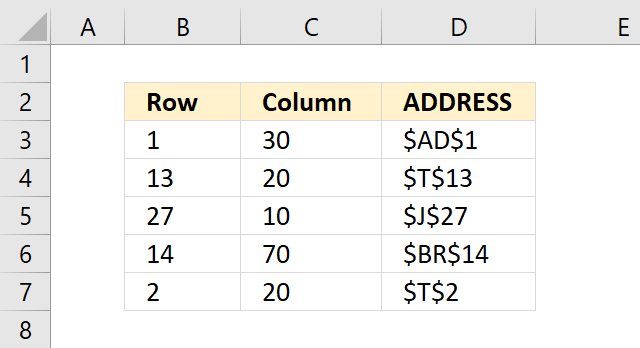
3. Example

Formula in cell D3:

The formula returns the address of a cell based on the row number in cell B3 and the column number in cell C3. The address is returned as an absolute reference in A1 style by default. For example, if B3 contains 1 and C3 contains 30, the formula returns $AD$1.

You can change the type of reference and the style of the address by adding optional arguments to the formula.
For example, =ADDRESS(B3, C3, 4) returns a relative reference (G5),
and =ADDRESS(B3, C3, 1, FALSE) returns an absolute reference in R1C1 style.

Back to top

3.1 Explaining formula

Step 1 - ADDRESS Function

The ADDRESS function calculates the address of a specific cell based on a row and column number.

ADDRESS(row_num, column_num, [abs_num], [a1], [sheet_text])

Step 2 - Populate arguments

ADDRESS(row_num, column_num, [abs_num], [a1], [sheet_text])

row_num - B3

column_num - C3

[abs_num], - optional

[a1] - optional

[sheet_text]) - optional

Step 3 - Evaluate ADDRESS function

ADDRESS(1, 30)

and returns "$AD$1". This is a string, not a cell reference.

Back to top

4. Function not working

Make sure your spelling is correct, the image above shows a #NAME! error in cell D3. The ADDRESS function is misspelled.

The image above shows a #VALUE! error, the second argument expects a cell reference or a number, however, a text string is used.

4.1 Troubleshooting the error value

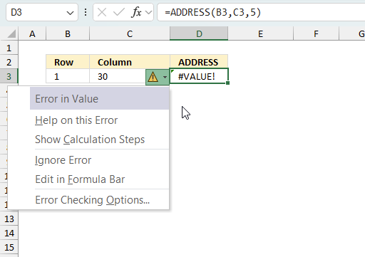
When you encounter an error value in a cell a warning symbol appears, displayed in the image above. Press with mouse on it to see a pop-up menu that lets you get more information about the error.

1. The first line describes the error if you press with left mouse button on it.
2. The second line opens a pane that explains the error in greater detail.
3. The third line takes you to the "Evaluate Formula" tool, a dialog box appears allowing you to examine the formula in greater detail.
4. This line lets you ignore the error value meaning the warning icon disappears, however, the error is still in the cell.
5. The fifth line lets you edit the formula in the Formula bar.
6. The sixth line opens the Excel settings so you can adjust the Error Checking Options.

Here are a few of the most common Excel errors you may encounter.

#NULL error - This error occurs most often if you by mistake use a space character in a formula where it shouldn't be. Excel interprets a space character as an intersection operator. If the ranges don't intersect an #NULL error is returned. The #NULL! error occurs when a formula attempts to calculate the intersection of two ranges that do not actually intersect. This can happen when the wrong range operator is used in the formula, or when the intersection operator (represented by a space character) is used between two ranges that do not overlap. To fix this error double check that the ranges referenced in the formula that use the intersection operator actually have cells in common.

#SPILL error - The #SPILL! error occurs only in version Excel 365 and is caused by a dynamic array being to large, meaning there are cells below and/or to the right that are not empty. This prevents the dynamic array formula expanding into new empty cells.

#DIV/0 error - This error happens if you try to divide a number by 0 (zero) or a value that equates to zero which is not possible mathematically.

#VALUE error - The #VALUE error occurs when a formula has a value that is of the wrong data type. Such as text where a number is expected or when dates are evaluated as text.

#REF error - The #REF error happens when a cell reference is invalid. This can happen if a cell is deleted that is referenced by a formula.

#NAME error - The #NAME error happens if you misspelled a function or a named range.

#NUM error - The #NUM error shows up when you try to use invalid numeric values in formulas, like square root of a negative number.

#N/A error - The #N/A error happens when a value is not available for a formula or found in a given cell range, for example in the VLOOKUP or MATCH functions.

#GETTING_DATA error - The #GETTING_DATA error shows while external sources are loading, this can indicate a delay in fetching the data or that the external source is unavailable right now.

4.2 The formula returns an unexpected value

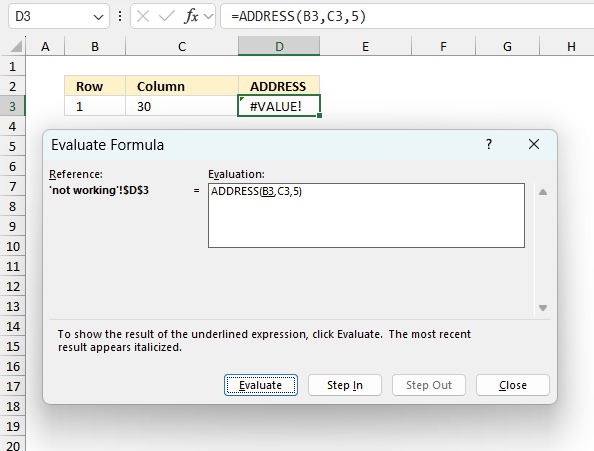
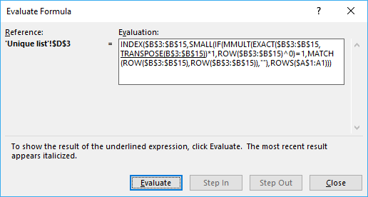
To understand why a formula returns an unexpected value we need to examine the calculations steps in detail. Luckily, Excel has a tool that is really handy in these situations. Here is how to troubleshoot a formula:

1. Select the cell containing the formula you want to examine in detail.
2. Go to tab “Formulas” on the ribbon.
3. Press with left mouse button on "Evaluate Formula" button. A dialog box appears.
   The formula appears in a white field inside the dialog box. Underlined expressions are calculations being processed in the next step. The italicized expression is the most recent result. The buttons at the bottom of the dialog box allows you to evaluate the formula in smaller calculations which you control.
4. Press with left mouse button on the "Evaluate" button located at the bottom of the dialog box to process the underlined expression.
5. Repeat pressing the "Evaluate" button until you have seen all calculations step by step. This allows you to examine the formula in greater detail and hopefully find the culprit.
6. Press "Close" button to dismiss the dialog box.

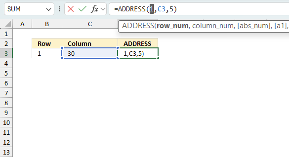
There is also another way to debug formulas using the function key F9. F9 is especially useful if you have a feeling that a specific part of the formula is the issue, this makes it faster than the "Evaluate Formula" tool since you don't need to go through all calculations to find the issue..

1. Enter Edit mode: Double-press with left mouse button on the cell or press F2 to enter Edit mode for the formula.
2. Select part of the formula: Highlight the specific part of the formula you want to evaluate. You can select and evaluate any part of the formula that could work as a standalone formula.
3. Press F9: This will calculate and display the result of just that selected portion.
4. Evaluate step-by-step: You can select and evaluate different parts of the formula to see intermediate results.
5. Check for errors: This allows you to pinpoint which part of a complex formula may be causing an error.

The image above shows cell reference B3 converted to hard-coded value using the F9 key, there is nothing wrong with this value however, the third argument is number 5. The ADDRESS function requires valid numbers between 1 and 4 which is not the case in this example. We have found what is wrong with the formula.

Tips!

• View actual values: Selecting a cell reference and pressing F9 will show the actual values in those cells.
• Exit safely: Press Esc to exit Edit mode without changing the formula. Don't press Enter, as that would replace the formula part with the calculated value.
• Full recalculation: Pressing F9 outside of Edit mode will recalculate all formulas in the workbook.

Remember to be careful not to accidentally overwrite parts of your formula when using F9. Always exit with Esc rather than Enter to preserve the original formula. However, if you make a mistake overwriting the formula it is not the end of the world. You can “undo” the action by pressing keyboard shortcut keys CTRL + z or pressing the “Undo” button

4.3 Other errors

Floating-point arithmetic may give inaccurate results in Excel - Article

Floating-point errors are usually very small, often beyond the 15th decimal place, and in most cases don't affect calculations significantly.

Back to top

5. Get value based on row and column number

Formula in cell D3:

The formula returns the value of the cell that has the address specified by the row number in cell B3 and the column number in cell C3. The ADDRESS function returns the address as a text string, and the INDIRECT function converts the text string into a valid reference. For example, if B3 contains 7 and C3 contains 3, the formula returns the value of cell C7.

You can use this formula to create a dynamic reference to a cell that changes based on the values in other cells.

5.1 Explaining formula

Step 1 - Calculate address

ADDRESS(B3, C3)

becomes

ADDRESS(7, 3)

and returns C7.

Step 2 - Convert string to cell reference

The INDIRECT function creates a cell reference from on a value.

INDIRECT(ref_text, [a1])

INDIRECT(ADDRESS(B3, C3))

becomes

INDIRECT("C7")

and returns "C".

Back to top

6. Get value based on row and column number - ADDRESS function alternative

I recommend the INDEX function instead of the ADDRESS and INDIRECT function to create a cell reference that you will be using to get a value. As I mentioned above, the INDIRECT function is volatile and I recommend avoiding volatile functions as much as possible.

Formula in cell D3:

The formula returns the value at the intersection of the row and column specified by the values in cells B3 and C3. The INDEX function takes a range or array as the first argument, and a row number and a column number as the second and third arguments. For example, if B3 contains 7 and C3 contains 3, the formula returns the value in cell C3. You can use this formula to look up values from a table or array based on numeric positions.

6.1 Explaining formula

Step 1 - INDEX function

The INDEX function returns

INDEX(reference, [row_num], [column_num], [area_num])

reference -
row_num -
column_num -
area_num - 

Step 2 - Populate arguments

INDEX(reference, [row_num], [column_num], [area_num])

reference - A1:E11
row_num - B3
column_num - C3
area_num - optional

Step 3 - Evaluate INDEx function

INDEX(A1:E11,B3,C3)

becomes

INDEX(A1:E11,7,3)

becomes cell reference C7

and returns "C".

Back to top

7. Get value based on a row and column number and a worksheet name

The image above demonstrates a formula in cell D3 that returns a value from another sheet using the ADDRESS function.

Formula in cell D3:

The formula above calculates the value of the cell that has the address specified by the row number in cell B3 and the column number in cell C3 on the worksheet named “ADDRESS function”. The ADDRESS function returns the address as an absolute reference in A1 style by default. The INDIRECT function converts the text string into a valid reference. For example, if B3 contains 3 and C3 contains 2, the formula returns the value of cell $B$3 on the worksheet “ADDRESS function”.

7.1 Explaining formula

Step 1 - ADDRESS function

The ADDRESS function calculates the address of a specific cell based on a row and column number.

ADDRESS(row_num, column_num, [abs_num], [a1], [sheet_text])

Step 2 - Populate arguments

row_num - B3

column_num - C3

[abs_num], - optional

[a1] - optional

[sheet_text]) - "ADDRESS function"

ADDRESS(row_num, column_num, [abs_num], [a1], [sheet_text])

becomes

ADDRESS(B3, C3, , , "ADDRESS function")

and returns 'ADDRESS function'!$B$3.

Step 3 - Create cell reference

The INDIRECT function creates a cell reference from on a value.

INDIRECT(ref_text, [a1])

INDIRECT(ADDRESS(B3, C3, , , "ADDRESS function"))

becomes

INDIRECT('ADDRESS function'!$B$3)

and returns 1.

Back to top

8. Create an address to a cell range and return values from that cell range

The image above shows a formula in cell E3 that creates a cell reference to a cell range using the ADDRESS function.

Array formula in cell E3:

The formula above calculates a reference to the range of cells that has the address specified by the row and column numbers in cells B3, C3, B4 and C4. The ADDRESS function returns the address as a text string, and the & operator concatenates the two addresses with a colon (:) to create a range reference. The INDIRECT function converts the text string into a valid reference.

For example, if B3 contains 8, C3 contains 2, B4 contains 9 and C4 contains 3, the formula returns a reference to the range $B$8:$C$9.

8.1 Explaining formula

Step 1 - Top left cell

ADDRESS(B3,C3)

becomes

ADDRESS(8,2)

and returns string "B8".

Step 2 - Bottom right cell

ADDRESS(B4,C4)

becomes

ADDRESS(9,3)

and returns string "C9".

Step 3 - Create a cell address to a cell range

The ampersand character lets you concatenate text strings in an Excel formula.

ADDRESS(B3,C3)&":"&ADDRESS(B4,C4)

becomes

B8&":"&C9

and returns the string "B8:C9".

Step 4 - Create a cell reference

The INDIRECT function creates a cell reference from on a value.

INDIRECT(ref_text, [a1])

INDIRECT(ADDRESS(B3,C3)&":"&ADDRESS(B4,C4))

becomes

INDIRECT("B8:C9")

and returns cell reference B8:C9.

Back to top

9. Extract column letter - Excel 365

The image above shows a formula in cell B3 that extracts the column letters from a given cell reference, in this example BC465.

Excel 365 formula in cell B3:

The formula calculates the column letters only from a given cell reference.

Explaining formula

Step 1 - Get column number

The COLUMN function returns a number representing the column of a given cell reference counting from the left.

COLUMN(cell_ref)

COLUMN(BC465)

returns 55. Column BC465 is the 55th column counting from the left, see the image above.

Step 2 - Create cell address

ADDRESS(1,COLUMN(BC465),4)

ADDRESS(row_num, column_num, [abs_num], [a1], [sheet_text])

[abs_num] - Optional. Let's you choose the type of reference to return.
1 - Absolute.
2 - Absolute row, relative column.
3 - Absolute column, relative row.
4 - Relative.

ADDRESS(1,COLUMN(BC465),4)

becomes

ADDRESS(1,55,4)

and returns BC1.

Step 3 - Count characters

The LEN function returns a number representing the total amount of characters in a string.

LEN(str)

LEN(ADDRESS(1,COLUMN(BC465),4))-1

becomes

LEN("BC1")-1

becomes

3 - 1 equals 2.

Step 4 - Remove row number

The LEFT function extracts a specific number of characters always starting from the left.

LEFT(ADDRESS(1,COLUMN(BC465),4),LEN(ADDRESS(1,COLUMN(BC465),4))-1)

becomes

LEFT("BC1",2)

and returns "BC".

Step 5 - Shorten formula

The LET function lets you name intermediate calculation results which can shorten formulas considerably and improve performance.

LEFT(ADDRESS(1,COLUMN(BC465),4),LEN(ADDRESS(1,COLUMN(BC465),4))-1)

ADDRESS(1, COLUMN(BC465), 4) is repeated twice in the formula.

x - ADDRESS(1, COLUMN(BC465), 4)

LET(x, ADDRESS(1, COLUMN(BC465), 4), LEFT(x, LEN(x)-1))

Back to top

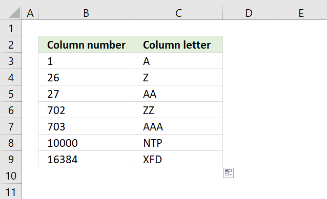
10. Convert column number to column letter

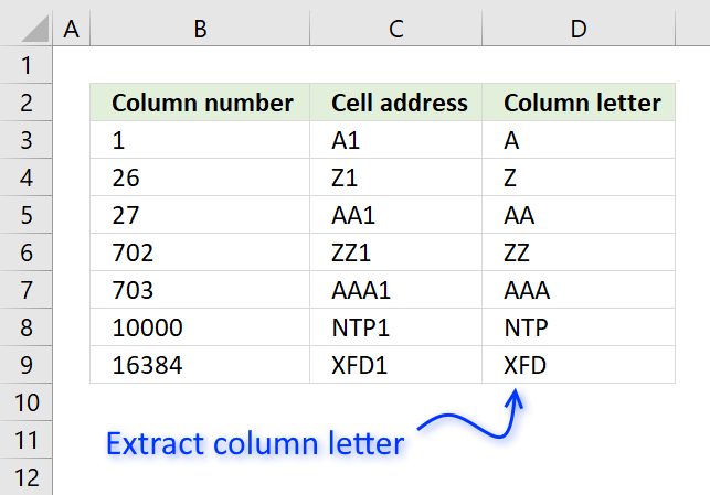
Use the following formula to convert a column number to a column letter:

The formula is entered in cell D3 shown in the image above, the column number is in cell B3.

Explaining formula in cell D3

You can follow along if you start the "Evaluate Formula" tool. You will find it on tab "Formula" on the ribbon.

Press with left mouse button on "Evaluate" button to move to the next calculation step.

Step 1 - Create a relative cell reference based on row and column number

The ADDRESS function returns a cell reference depending on what you use in the first (row) and second (column) argument.

The third argument lets you choose the type of cell reference the ADDRESS function returns. 4 is a relative cell reference.

ADDRESS(1, B3, 4)

becomes

ADDRESS(1, 1, 4)

and returns A1.

Step 2 - Remove last characters based on column number

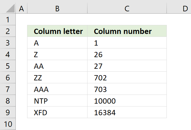
The column letters start with A and ends with XFD. A is column 1, AA is column 27, the first column reference that contains two letters.

AAA is the first column containing 3 letters and the corresponding column number is 703.

The MATCH function returns the position in the array of the largest value that is smaller than the lookup value (B3).

MATCH(B3, {1; 27; 703})

becomes

MATCH(1, {1; 27; 703})

and returns 1. The cell reference must have a single column letter.

Step 3 - Extract a given number of characters from the start of the string

LEFT(ADDRESS(1, B3, 4), MATCH(B3, {1; 27; 703}))

becomes

LEFT("A1", 1)

and returns A in cell D3.

11. Convert column letter to column number

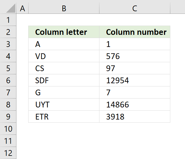
The following formula converts a column letter to the corresponding column number.

Formula in cell C3:

If you don't want to use the INDIRECT function because it is volatile and may cause your worksheet to slow down considerably if used extensively, use this array formula.

If you rather use a regular formula, try this:

Explaining formula in cell C3

Step 1 - Create a cell reference from a text string

The ampersand character & concatenates the value in cell B3 with 1.

The INDIRECT function converts the text string to a cell reference.

INDIRECT(B3&"1")

becomes

INDIRECT("A"&"1")

becomes

INDIRECT("A1")

and returns A1.

Step 2 - Return column from cell reference

COLUMN(INDIRECT(B3&"1"))

becomes

COLUMN(A1)

and returns 1 in cell C3.

12. Convert column number to column letter (VBA)

User defined function in cell C3:

VBA code

Function ColumnLetter(col As Integer) As String
ColumnLetter = Split(Cells(1, col).Address, "$")(1)
End Function

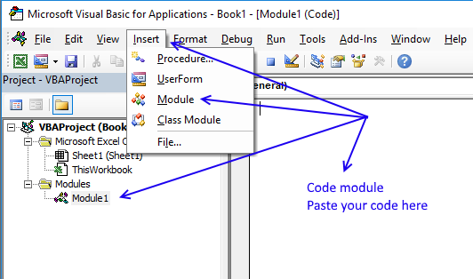
Where to copy the code?

1. Copy above custom function
2. Go to VBA Editor (Alt+F11)
3. Press with left mouse button on "Insert" on the top menu
4. Press with left mouse button on "Module" to insert a module to your workbook
5. Paste code into the code window
6. Exit VBA Editor and return to Excel (Alt+Q)

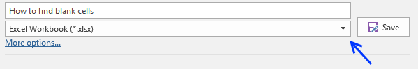
Save your workbook

To be able to use the user defined function next time you open your workbook you need to save the workbook as a macro-enabled workbook.

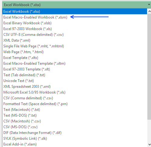
1. Press with left mouse button on "File" on the menu, or if you have an earlier version of Excel, press with left mouse button on the office button.
2. Press with left mouse button on "Save As"
3. Press with left mouse button on file extension drop-down list
   
4. Change the file extension to "Excel Macro-Enabled Workbook (*.xlsm)".
   

13. Convert column letter to column number (VBA)

User defined function in cell C3:

VBA code

Function ColumnNumber(col As String) As Long
ColumnNumber = Columns(col).Column
End Function

Get Excel *.xlsm file

Convert column number to column letter.xlsm

Useful resources

ADDRESS function - Microsoft
ADDRESS Function Examples - Contextures