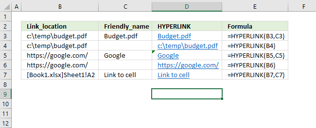
How to use the HYPERLINK function

What is the HYPERLINK function?
The HYPERLINK function allows you to build a link in a cell pointing to something else like a file, workbook, cell, cell range, or webpage.
You can then press with left mouse button on that link to open a file or quickly navigate to a location in a workbook.
Table of Contents
- Syntax
- Arguments
- How to select a cell containing a hyperlink?
- Function not working
- How to create a link to a cell
- How to create a link to a cell range
- How to create a link to another worksheet
- How to create a link to a workbook
- How to create a link to a named range
- How to create a link to an Excel Table
- How to create a link to a file
- How to create a link to a webpage
- How to create a link based on cell value
- Get Excel file
- Locate lookup values in an Excel table
- Navigate to first empty cell using a hyperlink formula
- Easily select data using hyperlinks
- Get the largest/smallest number
- Get the column header name that contains the largest/smallest value
- Get the cell address of the largest/smallest number
- Create a link to the largest/smallest number
- How to highlight the largest and smallest value
1. Syntax
HYPERLINK(link_location, [friendly_name])
2. Arguments
| Link_location | Required. Depending on what you want to create a link to you have these options:
|
| friendly_name | Optional. A value or a cell reference used by the HYPERLINK function to show link text, in the cell. This argument is optional, the HYPERLINK function displays the link location if the argument is missing. |
3. How to select a cell containing a link?
To select a cell without performing the hyperlink action press and hold on the cell until a cross appears, see the animated image above.
4. Function not working
The HYPERLINK functions first argument is not easy to type, there are a few things to remember:
- full path if the workbook or file is not in the same directory as the active workbook
- workbook name with leading and trailing bracket
- worksheet name with leading and trailing single quote if the name contains a space character
- exclamation mark between worksheet name and cell address
Below are common errors described.
4.1 Reference isn't valid error

The image above shows an error that Excel returns if the worksheet name is missing or the worksheet name contains space characters.
HYPERLINK(link_location, [friendly_name])
The link_location argument must contain a reference to the workbook name, worksheet name, exclamation mark between worksheet name and cell address, and a cell address if you want to link to an item in a workbook.
Formula in cell B3 that returns an error:
Worksheet reference "Link to a cell" above contains space characters, use a leading and trailing single quote or apostrophe to avoid the "Reference isn't valid" error.
Formula in cell B3 that works:
4.2 Cannot open the specified file error

The image above demonstrates an error that is returned if the workbook name is missing in the link_location argument.
HYPERLINK(link_location, [friendly_name])
Formula in cell B3 that returns an error:
The link_location argument above doesn't contain a reference to the workbook name, use leading and trailing brackets to avoid "Cannot open the specified file" error.
Formula in cell B3 that works:
4.3 Excel found a problem with one or more formula references in this worksheet

The image above shows an Excel error if the first argument in the HYPERLINK function is not correct.
The dialog box shows "Excel found a problem with one or more formula references in this worksheet. Check that the cell references, range names, defined names, and links to other workbooks in your formulas are all correct.
Formula in cell B3 that returns an error:
The link_location argument above doesn't contain a reference to a cell.
Formula in cell B3 that works:
5. How to create a link to a cell

The image above demonstrates how to link to a specific cell using the HYPERLINK function.
Formula in cell B3:
HYPERLINK(link_location, [friendly_name])
The link_location argument must contain a reference to the workbook, worksheet, and cell address. [friendly_name] argument lets you specify the hyperlink text to show in the cell.
Note the exclamation mark between the worksheet and cell address.
6. How to create a link to a cell range

The image above demonstrates how to link to a specific cell range using the HYPERLINK function. The cell range is selected if you press with left mouse button on the hyperlink.
Formula in cell B3:
HYPERLINK(link_location, [friendly_name])
The link_location argument must contain a reference to the workbook, worksheet, and a reference to a cell range. [friendly_name] argument lets you specify the hyperlink text to show in the cell.
Note the exclamation mark between the worksheet and cell address.
7. How to create a link to another worksheet

The image above demonstrates how to link to a specific worksheet using the HYPERLINK function.
Formula in cell B3:
HYPERLINK(link_location, [friendly_name])

8. How to create a link to a workbook

The image above demonstrates how to link to a specific workbook using the HYPERLINK function.
Formula in cell B3:
HYPERLINK(link_location, [friendly_name])
Note that a reference to the workbook name only is valid. Remember to reference the full path if the workbook is not in the same directory.
=HYPERLINK("[TEXT function.xlsx]","Link to Text function.xlsx")
9. How to create a link to a named range

The image above demonstrates how to link to a specific named range using the HYPERLINK function.
Formula in cell B3:
HYPERLINK(link_location, [friendly_name])
You need to specify the path, workbook name, and the name of the named range, the example above has no path specified. The workbook is in the same folder as the active workbook.
Read more about named ranges: Define and use names in formulas
10. How to create a link to an Excel Table

The image above demonstrates how to link to a specific named range using the HYPERLINK function.
Formula in cell B3:
HYPERLINK(link_location, [friendly_name])
You need to specify the path, workbook name, and the name of the Excel Table. The example above has no path specified, the workbook is in the same folder as the active workbook.
Read more about Excel Tables
11. How to create a link to a file

The image above shows how to link to a specific file using the HYPERLINK function.
Formula in cell B3:
HYPERLINK(link_location, [friendly_name])
You need to specify the path, file name, and file extension. The example above links to a pdf file named temp.pdf in a temp folder on harddrive c:\.
12. How to create a link to a webpage

The image above shows how to link to a specific website using the HYPERLINK function.
Formula in cell B3:
HYPERLINK(link_location, [friendly_name])
You need to specify the url to the website you want to link. The example above links to Google.
13. How to create a link based on cell value
If you use a cell reference as an argument you can make the function dynamic. This allows the HYPERLINK function to change depending on the value in the cell that the cell reference points to.
Formula in cell D3:
You can create formulas that lookup a value and return a link to that value using this technique.
Here are some articles:
Locate lookup values in an Excel table [HYPERLINK]
Navigate to first empty cell using a hyperlink formula
Create a hyperlink linked to the result of a two-dimensional lookup
How to quickly find the maximum or minimum value [Formula]
Useful resources
HYPERLINK function - Microsoft support
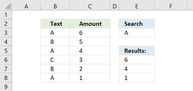
15. Locate lookup values in an Excel Table
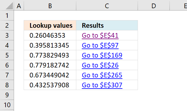
This section demonstrates a formula that returns a hyperlink pointing to a location based on a lookup value. When you press with left mouse button on the cell that contains the hyperlink text, Excel takes in an instant to that location in the table.
The formula is dynamic meaning if you change the search value the formula changes the location and the hyperlink text instantly.
Formula in cell C3:
This formula finds only the first instance of the search value, se further down the article for a formula that returns multiple results.
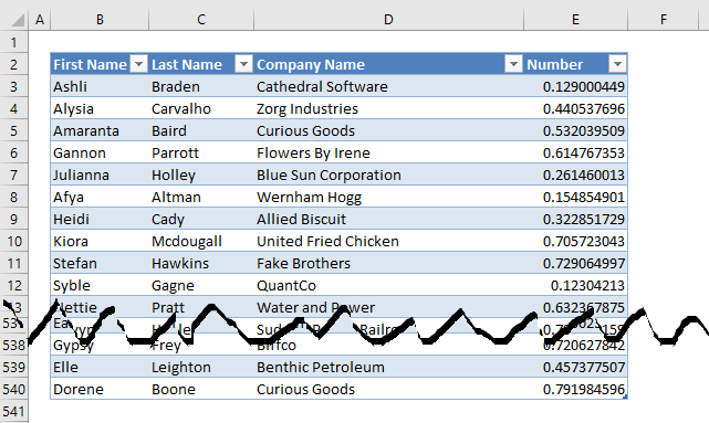
The Excel defined Table is located on worksheet "Table", the image above shows some records of that Excel defined Table.
Explaining formula in cell C3
I recommend you use the "Evaluate Formula" feature in Excel to examine calculations step by step.
Select cell C3, go to tab "Formulas" on the ribbon and press with left mouse button on the "Evaluate Formula" button.
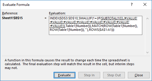
(The formula shown in the above image is not the formula used in this article.)
Press with left mouse button on "Evaluate" button to see the next step in the formula calculations.
Step 1 - Return the relative position of an item in an array that matches a specified value
The MATCH function returns the relative position of a value in a column.
MATCH(A2, Table1[Number], 0)
becomes
MATCH(0.260463529541505, {0.129000449044708;0.440537695535749;0.532039509437168; ...}, 0)
(Array shortened)
and returns 39.
Step 2 - Create a cell reference as text
The ADDRESS function returns a cell reference based on a row and column number. ADDRESS(row_num, column_num, [abs_num], [a1], [sheet_text])
ADDRESS(MATCH(A2, Table1[Number], 0)+MIN(ROW(Table1[Number]))-1, 5)
becomes
ADDRESS(39+MIN(ROW(Table1[Number]))-1, 5)
The MATCH function returns a relative position, it does not take into account cells above the Excel Table. We need to determine how many cells are above the Excel Table.
ADDRESS(39+MIN(ROW(Table1[Number]))-1, 5)
becomes
ADDRESS(39+MIN(3)-1, 5)
becomes
ADDRESS(41, 5)
The second argument is the column number and is hardcoded into the formula, you must change this to the column number to a number representing the column you search.
ADDRESS(41, 5)
and returns $E$41
Step 3 - Create a shortcut to a cell in sheet Table
The HYPERLINK function lets you build a hyperlink in a cell. It has the following arguments: HYPERLINK(link_location, [friendly_name])
HYPERLINK("[Find values quickly.xlsx]Table!"&ADDRESS(MATCH(A2, Table1[Number], 0)+MIN(ROW(Table1[Number]))-1, 5), "Go to "&ADDRESS(MATCH(A2, Table1[Number], 0)+MIN(ROW(Table1[Number]))-1, 5))
becomes
=HYPERLINK("[Find values quickly.xlsx]Table!$D$41, "Go to $D$41")

The animated image above shows what happens when you press with left mouse button on a hyperlink, note that the lookup value match the number.
What if there are multiple values matching your lookup value?
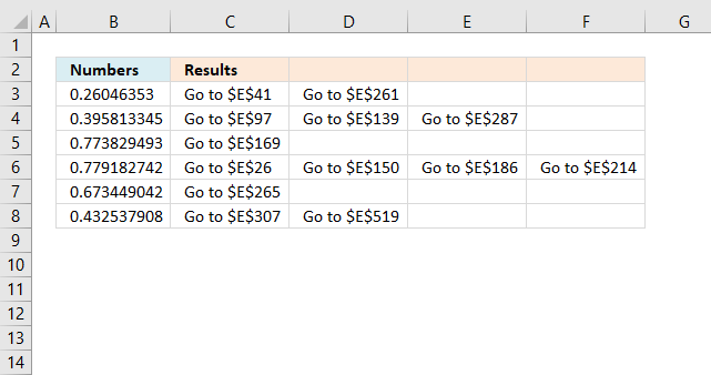
Array formula in cell C3:
How to create an array formula
- Copy above array formula
- Select cell B2
- Press with left mouse button on in formula bar

- Paste array formula
- Press and hold Ctrl + Shift
- Press Enter
How to copy array formula
- Select cell B2
- Copy cell (Ctrl + c)
- Select cell range C2:E2
- Paste (Ctrl + v)
- Select cell range B2:E2
- Copy (Ctrl + c)
- Select cell range B3:E7
- Paste (Ctrl + v)
Explaining formula in cell B2
Step 1 - Check if a condition is met and return corresponding row value if TRUE
IF($A2=Table1[Number], ROW(Table1[Number]), "")
becomes
IF(0.260463529541505={0.129000449044708;0.440537695535749;0.532039509437168; ...}, {3, 4, 5, ...}, "")
and returns
{""; ""; ""; ""; ""; ""; ""; ""; ""; ""; ""; ""; ""; ""; ""; ""; ""; ""; ""; ""; ""; ""; ""; ""; ""; ""; ""; ""; ""; ""; ""; ""; ""; ""; ""; ""; ""; ""; 41; ... ; ""} (Array shortened)
Step 2 - Return the k-th smallest value
SMALL(array, k)
SMALL(IF($A2=Table1[Number], ROW(Table1[Number]), ""), COLUMNS($A$1:A1))
becomes
SMALL({""; ""; ""; ""; ""; ""; ""; ""; ""; ""; ""; ""; ""; ""; ""; ""; ""; ""; ""; ""; ""; ""; ""; ""; ""; ""; ""; ""; ""; ""; ""; ""; ""; ""; ""; ""; ""; ""; 41; ... ""}, 1)
and returns 41.
Step 3 - Create a shortcut to a cell in sheet Table
HYPERLINK("[Find values quickly.xlsx]Table!"&ADDRESS(SMALL(IF($A2=Table1[Number], ROW(Table1[Number]), ""), COLUMNS($A$1:A1)), 4), "Go to "&ADDRESS(SMALL(IF($A2=Table1[Number], ROW(Table1[Number]), ""), COLUMNS($A$1:A1)), 4))
returns
HYPERLINK("[Find values quickly.xlsx]Table!$D$41, "Go to $D$41)
16. Navigate to first empty cell using a hyperlink formula

This article will demonstrate how to create a hyperlink that takes you to the first empty cell below data in a column. The way it works is that the Excel user press with left mouse button ons on the hyperlink and Excel instantly takes you to the first empty cell in a column.
The image above shows the formula in cell C2, it creates a hyperlink pointing to the first empty cell below the data set. This means that if more values are added to the data set the formula adapts and changes the destination cell making it dynamic without any user interaction.
This method can make the worksheet more user-friendly and easier to navigate, there is no VBA code or User Defined Functions in this workbook.
Formula in cell C2:

The hyperlink takes you to the first empty cell below the data set even if you have one or many blanks in the data set. The animated image above demonstrates this, the data set is not large in this example but you get the idea.
Explaining the formula in cell C2

I recommend using the "Evaluate Formula" tool which is a feature built-in to Excel. It allows you to see the formula calculation step by step.
Go to tab "Formulas" on the ribbon, press with left mouse button on the "Evaluate Formula" button and a dialog box opens, see image above.
The step that is about to be calculated is underlined, when you press with left mouse button on the "Evaluate" button the underlined expression is calculated. The calculated step is in italic.
Use the scroll arrows if the formula is larger than the window, this lets you see the entire formula. I wish it was possible to make that evaluation window larger though.
Press with left mouse button on the "Evaluate" button to move to the next step in the calculation. Continue press with left mouse button oning the "Evaluate" button to see all calculation steps in the formula. Press with left mouse button on "Close" button to dismiss the dialog box.
Step 1 - Find the last nonempty cell in cell range B1:B100
The CHAR function converts a number to the corresponding character based on your computer's character set. The numbers can be from 1 to 255 and they represent a character.
MATCH(CHAR(255),B1:B100,1)
becomes
MATCH(ÿ,B1:B100,1)
The MATCH function returns the relative position of a given value in a cell range. The third argument lets you choose how the function matches the value. Number 1 let you find the smallest value that is greater than or equal to the lookup value.
MATCH(lookup_value, lookup_array, [match_type])
We are looking for the last character in your computer's character set and it will most likely not be found. This will match the last value in your lookup_array even if it is not sorted in ascending order.
If you know that your lookup_array contains this value then I recommend using multiple values concatenated like this CHAR(255)&CHAR(255).
MATCH(ÿ,B1:B100,1)
and returns 8 which is the last value in cell range B1:B100.
If your data set has more than 100 rows use a larger cell range. For example B1:B1000 or the entire column B:B, however, the formula will probably run slower.
Step 2 - Join file name, sheet and cell address
The HYPERLINK function requires the file name, worksheet name and a cell reference to work properly. Step 1 above calculated the row number of the last non-empty cell.
We need to add the file name, worksheet name and column letter, then concatenate this string with the row number. The workbook name has a beginning and ending bracket characters and the worksheet name ends with a ! (exclamation mark).
We need to reference the first empty cell below the last non-empty value, in order to do that we add 1 to the calculated row number.
"[Quickly jump to last row using hyperlinks.xlsx]Sheet1!$B$"&MATCH(CHAR(255),B1:B100,1)+1
becomes
"[Quickly jump to last row using hyperlinks.xlsx]Sheet1!$B$"&8+1
and returns
[Quickly jump to the last row using hyperlinks.xlsx]Sheet1!$B$9
Step 3 - Create the hyperlink
The HYPERLINK function lets you build a hyperlink in your worksheet using a formula. A formula can be made dynamic so if your data set changes the formula changes as well without any user interaction.
HYPERLINK(link_location, [friendly_name])
The HYPERLINK function has two arguments, the first one is the link location. We built the link location in step 1 and 2. The friendly name is optional, I chose the word "Hyperlink". However, I recommend you use something more descriptive.
HYPERLINK("[Quickly jump to last row using hyperlinks.xlsx]Sheet1!$B$"&MATCH(CHAR(255),B1:B100,1)+1,"Hyperlink")
becomes
HYPERLINK([Quickly jump to last row using hyperlinks.xlsx]Sheet1!$B$9,"Hyperlink")
Tip 1

You can also use this keyboard shortcut to find the last non-empty cell:
- Select any cell in the column.
- Ctrl + Arrow key down.
However, if there are many blanks in your column you must repeatedly press the short cut keys to reach the last one.

Go to a column that has no values, press CTRL + arrow key down. This takes you to the last cell in that column. Use the arrow keys or your mouse to select any cell in the column you want to find the last value in.
Now press CTRL + arrow key up and Excel takes you to the last non-empty cell in that column.
Recommended reading
- Excel Hyperlinks and Hyperlink Function (Contextures)
- HYPERLINK function (Office support)
- Get workbook name (Formula)
- Get worksheet name (Formula)
17. Easily select data using hyperlinks

The image above shows two hyperlinks, the first hyperlink lets you select a data set automatically based on a dynamic formula. The second hyperlink takes you to a specific Excel Table and automatically selecting all data as well.
The technique demonstrated in this article will be interesting for you if you often copy data sets or Excel defined tables. Adding more rows or columns to the data set makes no difference, both the first formula and the Excel defined Table formula are dynamic meaning they adapt when lists grow or shrink. This may be a time-saver for you making some actions less tedious.
Formula in cell B3:
17.1 Explaining formula in cell B3

I recommend that you use the "Evaluate Formula" tool built-in to Excel. Go to tab "Formulas" on the ribbon and press with left mouse button on the "Evaluate Formula" button, a dialog box appears. Press with mouse on the "Evaluate" button to see calculations step by step, see image above.
The underlined expression tells you which part of the formula that will be calculated in the next step if you press the "evaluate" button. The result is in italic making it easier for you to understand and learn how a formula works. Press with left mouse button on "Close" button to dismiss the dialog box.
Step 1 - Find last row in the data set

The CHAR function converts a number to the corresponding character based on your computer's character set. The numbers can be from 1 to 255 and they represent a character.
MATCH(CHAR(255), Sheet2!B1:B1000, 1)
becomes
MATCH("ÿ", Sheet2!B1:B1000, 1)
The MATCH function returns a number representing the relative position of a given value in a cell range. The third argument lets you choose how the function matches the value. Number 1 lets you find the smallest value that is greater than or equal to the lookup value.
MATCH(lookup_value, lookup_array, [match_type])
The formula is looking for the last character in your computer's character set and it will most likely not be found. This will match the last value in your lookup_array. It is not required to have the column sorted in ascending order.
I recommend using multiple values concatenated like this CHAR(255)&CHAR(255) if you know that your lookup_array contains CHAR(255) .
MATCH("ÿ", Sheet2!B1:B1000, 1)
an returns 102.
Change cell range B1:B1000 if the data set has more than a thousand rows or if the data set location requires you to change the cell reference.
Step 2 - Find the rightmost column in the data set

The MATCH function returns the relative position of a given value in a cell range. It lets you choose how the function matches the value, use 1 in the third argument. It allows you to find the smallest value that is greater than or equal to the lookup value.
MATCH(lookup_value, lookup_array, [match_type])
We are looking for the last character in your computer's character set and it will most likely not be found. This will match the last value in your lookup_array even if it is not sorted in ascending order.
MATCH(CHAR(255), Sheet2!A2:CW2, 1)
returns 5.
This number represents the rightmost column in the data set. Change cell range A2:CW2 if the data set has more than a hundred columns.
Step 3 - Create cell reference
The ADDRESS function returns the address of a specific cell, based on a row and column number. We calculated the row and column numbers in steps 1 and 2.
ADDRESS(row_num, column_num, [abs_num], [a1], [sheet_text])
[abs_num], [a1], and [sheet_text] are optional arguments that we don't need to use in this tutorial.
ADDRESS(MATCH(CHAR(255), Sheet2!B1:B1000, 1), MATCH(CHAR(255), Sheet2!A2:CW2, 1))
becomes
ADDRESS(102, 5)
returns cell reference $E$102.
Step 4 - Add file and sheet name
The HYPERLINK function requires the workbook name and worksheet name to operate properly. The ampersand character lets you concatenate two strings, in this case, the workbook name, the worksheet name, and the cell reference.
The workbook name must have a beginning and ending bracket and ther worksheet name must end with an exclamation mark.
"[Quickly select a data set or an excel defined table.xlsx]Sheet2!$B$2:"&ADDRESS(MATCH(CHAR(255), Sheet2!B1:B1000, 1), MATCH(CHAR(255), Sheet2!A2:CW2, 1))
becomes
"[Quickly select a data set or an excel defined table.xlsx]Sheet2!$B$2:"&$E$102)
becomes
[Quickly select a data set or an excel defined table.xlsx]Sheet2!$B$2:$E$102
Step 5 - Create the hyperlink
The HYPERLINK function lets you build a hyperlink in your worksheet using a formula. A formula can be made dynamic so if your data set changes the formula changes as well without any user interaction.
HYPERLINK(link_location, [friendly_name])
HYPERLINK("[Quickly select a data set or an excel defined table.xlsx]Sheet2!$B$2:"&ADDRESS(MATCH(CHAR(255), Sheet2!B1:B1000, 1), MATCH(CHAR(255), Sheet2!A2:CW2,1)), "sheet2")
becomes
HYPERLINK([Quickly select a data set or an excel defined table.xlsx]Sheet2!$B$2:$E$102, "sheet2")
Formula in cell B4:
17.2 Select Excel defined Table using a hyperlink

The Excel Table is great a built-in tool that has many advantages. This tutorial demonstrates how Excel uses cell references to Excel Tables. They are called "structured references" and work differently than regular cell references.
A structure reference begins with the Excel Table name, press with left mouse button on any cell in the Excel Table. Press with mouse on tab "Table Design" on the ribbon, the tab appears if you have a cell in the Excel Table selected. You can find the Table name on the ribbon, it also allows you to change the Table name if you want to.
The name box shown in the image above lets you try different "structured references" and see what they do. The table below shows different "structured references", type them in the name box and check out what Excel selects.
For example, you will select data in the Excel Table if you only reference the Excel Table name. Structured references allow you to also use square brackets as well to further specify data you want to reference in the Excel Table.
| Structured reference | Description |
| Table1[#All] | Selects everything, headers, and data. |
| Table1 | Selects data. |
| Table1[[#All],[Country]] | Selects data and column header "Country". |
| Table1[Country] | Selects data in column Country |
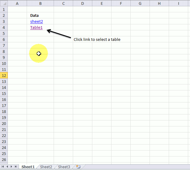
The animated gif shows two hyperlinks, the first one selects a data set, the second one selects an excel defined table.
18. Get the smallest number
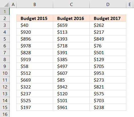
This article demonstrates formulas that will return the largest and smallest numbers, the corresponding column headers, the cell addresses, and how to link to their location as well as highlighting those values.
I will now demonstrate four different formulas, all regular formulas that will tell you something about where the largest and smallest values are. I will also show you a technique that highlights the smallest and largest value.
Get the largest/smallest number
The first formula returns the largest value from a cell range. The MAX function returns the largest number from a cell range.
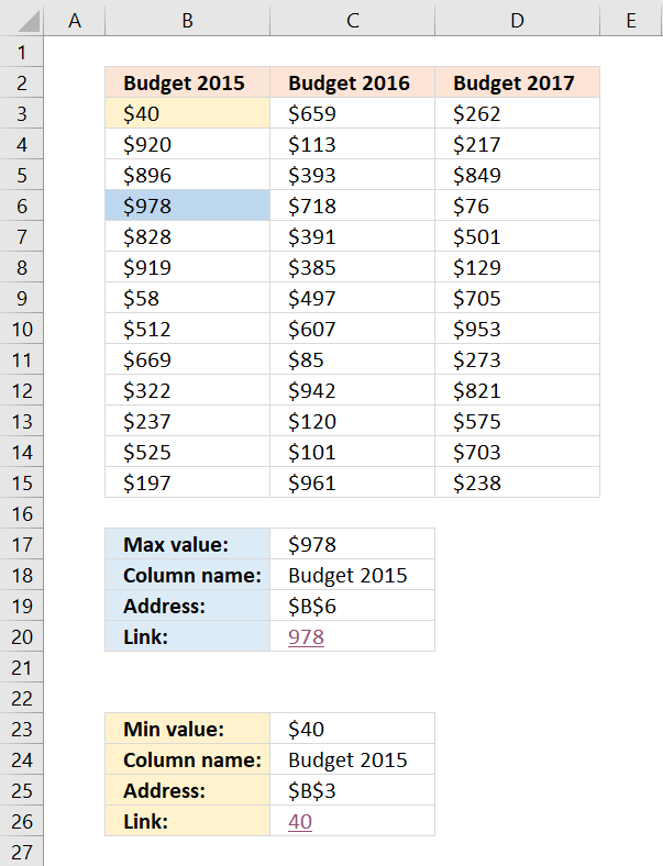
Formula in cell C17:
This formula returns the smallest number:
Explaining formula in cell C17
I am now going to explain the formula in cell C17: =MAX(B3:D15)
The MAX function returns the largest number in a cell range, you can also use multiple cell ranges, like this =MAX(B3:D15, F10:H22)
The MAX function allows you to have up to 255 arguments and it will ignore text and blank cells. However, if a cell contains an error value the function will also return an error value.
19. Get the column header name containing the largest/smallest number
The following formula returns the header name of the column that contains the largest value. I will explain these formulas later on, in this article.
Formula in cell C18:
This formula returns the column header of the smallest number
2.1 Explaining formula in cell C18
I am now going to explain the formula in cell C18.
Step 1 - Get the largest number in a given cell range
The MAX function returns the largest number from a cell range or array.
MAX(B3:D15)
returns 978.
Step 2 - Where is the largest value?
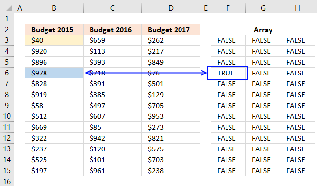
The following logical expression returns an array that displays the location of the maximum value. This part of the formula compares the largest value to each value and returns TRUE if equal and FALSE if not.
The equal sign lets you compare values not considering upper and lower letters, use the EXACT function if you need to do a case sensitive comparison. The result is either boolean value TRUE or FALSE.
$B$3:$D$15=MAX(B3:D15)
becomes
$B$3:$D$15=978
and returns {FALSE, FALSE, ... , FALSE}
The picture below shows the array in cell range F3:H15, the corresponding location in the array returns TRUE. Remaining values in the array show FALSE.
Step 3 - Convert TRUE value to a column number
The next step is to multiply the array with the corresponding column numbers.
($B$3:$D$15=MAX(B3:D15))* MATCH(COLUMN($B$3:$D$15), COLUMN($B$3:$D$15))
becomes
($B$3:$D$15=MAX(B3:D15))* {1,2,3}
and returns {0,... ,0}
The picture below displays the array in cell range F3:H15, The TRUE value now contains number 1 which is the relative column number in cell range B3:D15 for that location. In other words, the maximum value is found in the first column.
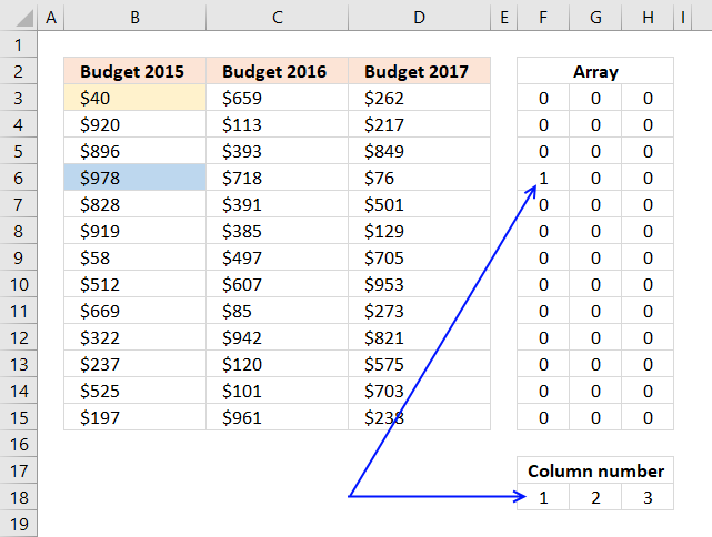
Step 4 - Sum values in the array
The SUMPRODUCT function lets you do these mathematical operations without the need to enter the formula as an array formula.
SUMPRODUCT(($B$3:$D$15=MAX(B3:D15))* MATCH(COLUMN($B$3:$D$15), COLUMN($B$3:$D$15)))
becomes
SUMPRODUCT({0,... ;1,....,0})
and returns 1.
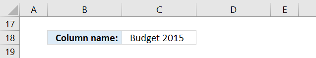
Step 5 - Return header name
The INDEX function fetches a value based on coordinates. Since the values are in a single row we need only to enter the argument for the column number.
INDEX(cell_ref, row_number, column_number)
INDEX($B$2:$D$2, ,SUMPRODUCT(($B$3:$D$15=MAX(B3:D15))* MATCH(COLUMN($B$3:$D$15), COLUMN($B$3:$D$15))))
returns Budget 2015 in cell C18.
What happens if there are two or more cells containing the largest number?
The formula won't work, the sum will not correspond to the column numbers.
20. Get the cell address of the largest number
This formula returns the address of the largest value, Excel has a grid with columns and rows. Example, address D16 is found in column D and row 16.
Formula in cell C19:
The following formula returns the address of the smallest number:
3.1 Explaining formula in cell C19
Step 1 to 4 calculate the row number used in the ADDRESS function and step 5 and 6 calculates the column number.
Step 1 - Get the largest number
The MAX function returns the largest number from a cell range or array.
MAX(B3:D15)
returns 978.
Step 2 - Identify where the largest number is
$B$3:$D$15=MAX(B3:D15)
becomes
$B$3:$D$15=978
becomes
{40, 659, 262; ... , 238}=978
and returns {FALSE, FALSE, FALSE; ... , FALSE}.
The arrays above are shorted, you can see the entire arrays in section 2.1.
Step 3 - Multiply with row numbers
The asterisk lets you multiply values, it works fine with boolean values as well as arrays.
($B$3:$D$15=MAX(B3:D15))* ROW($B$3:$D$15)
and returns {0, 0, ... , 0}.
The ROW function returns the row number of each row in B3:D15.
Step 4 - Sum numbers in array
The SUMPRODUCT function calculates the product of corresponding values and then returns the sum of each multiplication.
SUMPRODUCT(array1, [array2], ...)
SUMPRODUCT(($B$3:$D$15=MAX(B3:D15))* ROW($B$3:$D$15))
becomes
SUMPRODUCT({0, ... ;6, ... , 0})
and returns 6.
Step 5 - Calculate column number
I showed how to calculate the largest number and how to compare the number to array $B$3:$D$15 in step 1 and 2.
($B$3:$D$15=MAX(B3:D15))* COLUMN($B$3:$D$15))
returns {0, ... ;1, ... , 0}.
The COLUMN function returns a relative number for each column in cell range B3:B15.
Step 6 - Sum numbers in array
The SUMPRODUCT function calculates the product of corresponding values and then returns the sum of each multiplication.
SUMPRODUCT(array1, [array2], ...)
SUMPRODUCT(($B$3:$D$15=MAX(B3:D15))* COLUMN($B$3:$D$15))
becomes
SUMPRODUCT({0, ... ;1, ... , 0})
and returns 1.
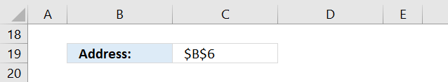
Step 7 - Get address based on row and column numbers
The ADDRESS function returns a cell reference as a text value, to be able to do that it needs to know the row and column number.
ADDRESS(row_number, column_number)
ADDRESS(SUMPRODUCT(($B$3:$D$15=MAX(B3:D15))* ROW($B$3:$D$15)), SUMPRODUCT(($B$3:$D$15=MAX(B3:D15))* COLUMN($B$3:$D$15)))
becomes
ADDRESS(6, 2)
and returns $B$6 in cell C19.
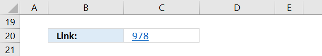
21. Create a link to the largest number
The next formula creates a hyperlink that allows you to quickly move to and select the largest value. You simply press with left mouse button on the cell and Excel instantly navigates to that cell, even if it is on another worksheet.
Formula in cell C20:
This formula returns a hyperlink pointing to the smallest number:
4.1 Explaining formula in cell C20
Step 1 - Calculate cell address
This part of the formula is already explained in section 3.1 above, check it out if you want a detailed explanation.
ADDRESS(SUMPRODUCT(($B$3:$D$15=MAX(B3:D15))* ROW($B$3:$D$15)), SUMPRODUCT(($B$3:$D$15=MAX(B3:D15))* COLUMN($B$3:$D$15)))
returns B6.
Step 2 - Create a hyperlink
This section explains the formula in cell C20. The HYPERLINK function allows you to create a link to a cell location. (It can do more than that but this is all you need to know for now.)
HYPERLINK(link_location, friendly_name)
The link location is a cell reference to a specific cell in your workbook. You need to specify the workbook name, worksheet name, and cell address. Read the previous explanation to learn how to calculate the cell reference of the maximum value.
HYPERLINK("[Min and max out of multiple columns.xlsx]Sheet1!"&ADDRESS(SUMPRODUCT(($B$3:$D$15=MAX(B3:D15))* ROW($B$3:$D$15)), SUMPRODUCT(($B$3:$D$15=MAX(B3:D15))* COLUMN($B$3:$D$15))), MAX(B3:D15))
becomes
HYPERLINK("[Min and max out of multiple columns.xlsx]Sheet1!"&B6, MAX(B3:D15))
The second argument is the value that you want the cell to show, in this case, the maximum value.
HYPERLINK("[Min and max out of multiple columns.xlsx]Sheet1!"&B6, MAX(B3:D15))
becomes
HYPERLINK("[Min and max out of multiple columns.xlsx]Sheet1!"&B6, 978)
and returns 978 (hyperlink) in cell C20.
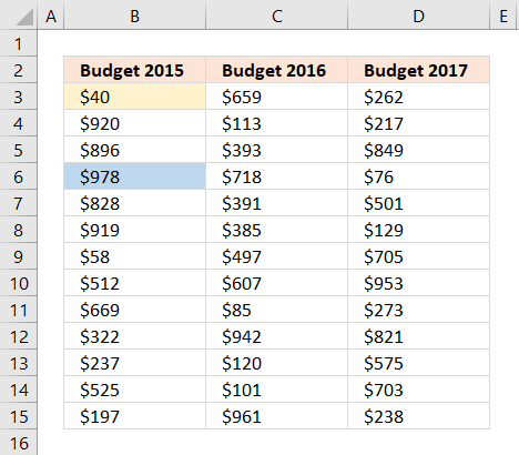
22. How to highlight the largest and smallest number
Conditional formatting allows you to format specific values using a formula or built-in criteria, in this case, I will highlight the cells containing the maximum and minimum value in a cell range.
- Select cell range B3:D15.
- Go to tab "Home" if you are not already there.
- Press with mouse on the "Conditional formatting" button.
- Press with left mouse button on "New Rule..".
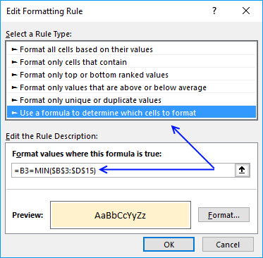
- Press with mouse on "Use a formula to determine which cells to format".
- Type this formula in field "Format values where this formula is true:": =B3=MAX($B$3:$D$15)
- Press with left mouse button on "Format..." button.
- Press with mouse on tab "Fill".
- Pick a color.
- Press with left mouse button on "OK" button.
- Press with left mouse button on "OK" button.
Repeat the above steps to highlight the minimum value using this formula: =B3=MIN($B$3:$D$15)
Remember to pick a different color.
Get Excel *.xlsx file
Min and max out of multiple columns.xlsx
'HYPERLINK' function examples
Table of Contents How to perform a two-dimensional lookup Reverse two-way lookups in a cross reference table [Excel 2016] Reverse […]
This article demonstrates how to work with multiple criteria using INDEX and MATCH functions. Table of Contents INDEX MATCH - […]
Functions in 'Lookup and reference' category
The HYPERLINK function function is one of 25 functions in the 'Lookup and reference' category.
Excel function categories
Excel categories
26 Responses to “How to use the HYPERLINK function”
Leave a Reply
How to comment
How to add a formula to your comment
<code>Insert your formula here.</code>
Convert less than and larger than signs
Use html character entities instead of less than and larger than signs.
< becomes < and > becomes >
How to add VBA code to your comment
[vb 1="vbnet" language=","]
Put your VBA code here.
[/vb]
How to add a picture to your comment:
Upload picture to postimage.org or imgur
Paste image link to your comment.
Ah there we go, I had some issues commenting on this before.
Firstly, thank you for these excellent examples, very helpful and instructive.
I'm an accountant and the second part of this article (hyperlinking to multiple matches) would be fantastically useful to me but unfortunately I usually work in a column format, not horizontally as the example shows.
Would you mind showing me how I would need to change the formula to reflect multiple matches in a single column. So that if columns C,D,E were cleared and A2 was repeated in say A4 and A5 then A4 would be the next match and say "Go to D260" (currently C2 as it is showing the matches horizontally). As there would be no further matches then A5 would be blank and then the matches for A6 would then continue vertically.
Thank you very much for your time and I hope you don't mind showing me how to achieve this result.
Kind regards,
Oliver
Oliver,
I am happy you like it!
Array formula in cell B2:
Get the Excel *.xlsx file
Find-values-quicklyv2.xlsx
Hi Oscar,
Thanks so very much for the reply. I had tried using countif but clearly I wasn't putting it in the right spot!
Above you've explained very clearly what is happening with the rows etc and so I'm quite happy with this, unfortunately I am having trouble tailoring this for my own purpose which is to not reference a table(Table1[Number]) but rather a sheet (Sheet5!D:D). Somehow when I change the references, something unexpected happens and the formula no longer functions quite the same. Would you be so kind as to show me the correct usage for this method?
So for instance if I had the same sort of numbers but in column D in say, Sheet5, not a table.
My other question is whether there is a method for achieving the same result in VBA. While I have seen many attempts at creating separate lists showing differences or matches, this is quite unique in that it allows for navigation of a table (which is more reflective of what a manual process would be if I had to tick through each match).
Thank you very much for your help,
Oliver
Oliver,
Change the table references to absolute cell references.
Example:
to
Note! COUNTIF($A$2:A2, A2) uses both relative and absolute cell references.
Hi Oscar,
Thanks so very much for the reply. I had tried using countif but clearly I wasn't putting it in the right spot!
Above you've explained very clearly what is happening with the rows etc and so I'm quite happy with this, unfortunately I am having trouble tailoring this for my own purpose which is to not reference a table(Table1[Number]) but rather a sheet (Sheet5!D:D). Somehow when I change the references, something unexpected happens and the formula no longer functions quite the same. Would you be so kind as to show me the correct usage for this method?
So for instance if I had the same sort of numbers but in column D in say, Sheet5, not a table.
My other question is whether there is a method for achieving the same result in VBA. While I have seen many attempts at creating separate lists showing differences or matches, this is quite unique in that it allows for navigation of a table (which is more reflective of what a manual process would be if I had to tick through each match).
Thank you very much for your help,
Oliver
hai oscar,
I have a table with customers as column & products as rows. Price may different to each customer and product. i am using the following formula to find out the rate of an item for a particular customer;
"=IF(INDEX(TABLE3,MATCH(REF_ID,INDEX(TABLE3,,1),0),MATCH(REF_prod,INDEX(TABLE3,1,),0))<=0,"PLEASE INSERT A RATE",(INDEX(TABLE3,MATCH(REF_ID,INDEX(TABLE3,,1),0),MATCH(REF_prod,INDEX(TABLE3,1,),0)))).
now i want to locate/hyperlink the particular cell intersecting the customer reference and product reference. can u pls help me
RAJ.A.D,
read this post: Locate a particular cell in a table
Oscar, I played around with this type of MATCH formula long ago and found it to be a little buggy. Noenetheless, I have found that the most general form of this formula is:
=MAX(MATCH(0,A:A,-1),MATCH(CHAR(255),A:A,1))
David Hager,
You are right, I remember sam´s comment now:
https://www.get-digital-help.com/create-a-dynamic-named-range-in-excel/#comment-24493
I am at a complete loss with this. This hyperlink function should work perfectly but it completely ignores the array that I program it to look within and returns me to a cell that is outside of the lookup array.
=HYPERLINK("[CompletePull.xlsx]'Sheet2'!$E$"&MATCH(410000,Sheet2!E3:E1002,1)+1,1)
I am attempting to match the entered date and return the cursor to the empty cell below on sheet two. My cursor returns to cell C1 instead. Would anyone tell me where I am going wrong here? My lookup array is clearly Sheet2 E3:E1002. Why would it even return my cursor to anything outside of that range?
=HYPERLINK("[CompletePull.xlsx]'Sheet2'!$E$"&MATCH(410000,Sheet2!E3:E1002,1)+3,1)
Okay, I have figured out how to get this syntax to work for dates. For some reason I had to tell the match formula to return the reference plus 3. I am having a hard time dissecting that but if anyone can help me with it, it would be much appreciated.
Thank you Oscar, I've been trying to figure this one out for a long time.
Randy,
MATCH(410000,Sheet2!E3:E1002,1)
Is your list sorted in an ascending order?
Read this:
[…] out Oscar Cronquist’s post about dynamic […]
Hello oscar
I wanted to use your formula and play a bit with it but the file doesn't seem to work when I got (error cant open the specific file when I press a hyperlink) now I wanted to know if it is possible to extend that the lookup value is now compared with the row number can be searched in 3 different rows? And also is it possible to do it over several sheets?
Hello,
How about if I am using open office?
Faith
Sorry, I don't know.
I have 18 columns and more than 40 rows data, and I want peak the largest value among and lookup the corespondent value (heading and field name) with the data,
I tray =index(array,match(lookup value, array, 0)) returns #N/A,
array assume from $C$4:$T$391
lookup value AH4,
esse
Can you post your formula, there seems to be nothing wrong with the one you provided.
You get a #N/A error if the lookup value is not found.
Awesome!, Thanks, you made my day, really relieved.
Oscar,
What is the best way to get around the characters limit when using HYPERLINK? Thanks
Oscar, let's use CELL("filename") to make a filename-sheetname part dynamic, so, combined with David's suggestion, it will look like: HYPERLINK(REPLACE(CELL("filename"),1,FIND("[",CELL("filename")),"[")&"!B"&MAX(MATCH(0,B:B,-1),MATCH(CHAR(255),B:B,1))+1,"HYPERLINK")
Leonid,
great comment.
Thank you!
What is wrong with the below formula? When I press with left mouse button on the hyperlink, the cursor stops at A2270. Tried out various options, yet cursor stops at A2270.
=HYPERLINK("[BANK STATEMENT.xlsx]ICICI$c$"&MATCH(CHAR(255),C2:C3000,1)+1,"BACK")Help !
Thanks,
Martin
Martin,
Perhaps there is a CHAR(255) character in C2270?
This article demonstrates a formula that extracts ANSI characters:
https://www.get-digital-help.com/identify-all-characters-in-a-cell-value/
I get the message " Cannot open the specified file"
Mark,
You need to enter the name of your workbook file in the formula:
[Find values quickly.xlsx]Table!
Find values quickly.xlsx is my file name.