Working with unique values
What's on this page
- Extract unique values from two columns - Excel 365
- Extract unique values from two columns - earlier Excel versions
- Filter unique values and sort based on adjacent date - Excel 365
- Filter unique values from a cell range - all Excel versions
- Filter unique values sorted from A to Z
- Find min and max unique and duplicate numerical values
- Filter unique strings from a cell range
- Extract a case sensitive unique list from a column
- Extract a case sensitive unique list from a column - Excel 365
1. Extract unique values from two columns - Excel 365
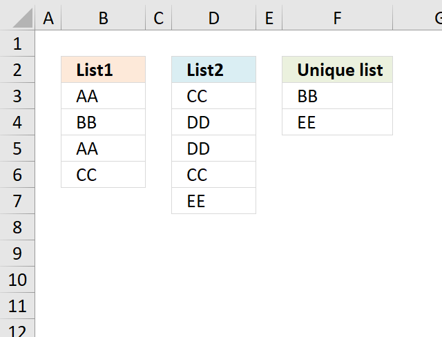
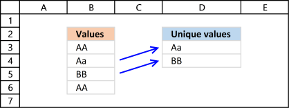
The image above demonstrates an Excel 365 formula in cell F3 that extracts unique values from two different columns. The columns are not adjacent and are not equal in size.
The first cell range B3:B6 contains "AA", "BB", "AA", and "CC". The second cell range D3:D7 contains "CC", "DD", "CC", and "EE". Unique values are "BB" and "EE" if you take both cell ranges into account.
Excel 365 dynamic array formula in cell F3:
This formula works only in Excel 365 and is entered as a regular formula despite its name. It spills values to cells below as far as needed.
The formula returns a #SPILL error if one or more cells are populated with characters. Delete the values and the formula spills values to cells below automatically.
Explaining formula in cell F3
Step 1 - Stack cell ranges vertically
The VSTACK function combines cell ranges or arrays. Joins data to the first blank cell at the bottom of a cell range or array (vertical stacking)
Function syntax: VSTACK(array1,[array2],...)
VSTACK(B3:B6, D3:D7)
becomes
VSTACK({"AA"; "BB"; "AA"; "CC"}, {"CC"; "DD"; "DD"; "CC"; "EE"})
and returns
{"AA"; "BB"; "AA"; "CC"; "CC"; "DD"; "DD"; "CC"; "EE"}
Step 2 - Extract unique values
The UNIQUE function returns a unique or unique distinct list.
Function syntax: UNIQUE(array,[by_col],[exactly_once])
UNIQUE(VSTACK(B3:B6, D3:D7),,1)
becomes
UNIQUE({"AA"; "BB"; "AA"; "CC"; "CC"; "DD"; "DD"; "CC"; "EE"},,1)
and returns
{"BB"; "EE"}.
2. Extract unique values from two columns - earlier Excel versions
I read an article Merging Lists To A List Of Distinct Values at CPearson. The article describes code that you can use to merge two lists into a third list and prevent duplicate entries in the resulting list, using VBA to create a macro.
Here is a solution to create a unique list from two columns without using VBA.
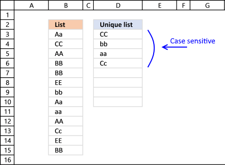
The picture below shows the unique list in column F.
The following formula returns values that are unique from two columns combined. Unique values are values that only exist once in both columns.
Formula in cell F3:
Explaining formula in cell F3
This formula may seem big, however, it is actually two smaller formulas combined. If you want to see the calculation steps then go to tab "Formulas" on the ribbon and press with left mouse button on "Evaluate Formula" button, then press with left mouse button on "Evaluate" button to move to next step in the calculation.
Step 1 - Prevent duplicate values
The COUNTIF function is really helpful in this situation, it counts the values in order to display unique values from two columns combined.
COUNTIF(F2:$F$2, $B$3:$B$6)
becomes
COUNTIF("Unique list", {"AA";"BB";"AA";"CC"})
and returns {0;0;0;0}.
Step - 2 - Count values in List1 against List 2
COUNTIF($D$3:$D$7, $B$3:$B$6)
becomes
COUNTIF({"CC";"DD";"DD";"CC";"EE"}, {"AA";"BB";"AA";"CC"})
and returns {0;0;0;2}. This tells us that only "CC" has a duplicate in List2.
Step 3 - Count values in List1
The following COUNTIF formula identifies unique values in cell range $B$3:$B$6
COUNTIF($B$3:$B$6, $B$3:$B$6)
becomes
COUNTIF({"AA";"BB";"AA";"CC"}, {"AA";"BB";"AA";"CC"})
and returns
{2;1;2;1}.
Step 4 - Add arrays
(COUNTIF(F2:$F$2, $B$3:$B$6)+COUNTIF($D$3:$D$7, $B$3:$B$6)+COUNTIF($B$3:$B$6, $B$3:$B$6))
becomes
{0;0;0;0} + {0;0;0;2} + {2;1;2;1}
equals
{2;1;2;3}.
Step 5 - Check if value in array is equal to 1
(COUNTIF(F2:$F$2, $B$3:$B$6)+COUNTIF($D$3:$D$7, $B$3:$B$6)+COUNTIF($B$3:$B$6, $B$3:$B$6))=1
becomes
{2;1;2;3}=1
and returns
{FALSE;TRUE;FALSE;FALSE}.
Step 6 - Divide 1 with array
1/((COUNTIF(F2:$F$2, $B$3:$B$6)+COUNTIF($D$3:$D$7, $B$3:$B$6)+COUNTIF($B$3:$B$6, $B$3:$B$6))=1)
becomes
1/({FALSE;TRUE;FALSE;FALSE})
and returns
{#DIV/0!;1;#DIV/0!;#DIV/0!}
Step 7 - Return value based on array
LOOKUP(2, 1/((COUNTIF(F2:$F$2, $B$3:$B$6)+COUNTIF($D$3:$D$7, $B$3:$B$6)+COUNTIF($B$3:$B$6, $B$3:$B$6))=1),$B$3:$B$6)
becomes
LOOKUP(2, {#DIV/0!;1;#DIV/0!;#DIV/0!},$B$3:$B$6)
becomes
LOOKUP(2, {#DIV/0!;1;#DIV/0!;#DIV/0!},{"AA";"BB";"AA";"CC"})
and returns "BB" in cell F3.
Step 8 - Return values from List 2
When the first formula returns errors the IFERROR function directs to the next formula. The next formula is exactly the same as the first formula except that it gets values from List 2.
=IFERROR(formula1, formula2)
Get excel sample file for this tutorial
unique list from two columnsv2.xlsx
3. Filter unique values and sort based on adjacent date - Excel 365

This example shows an Excel 365 formula in cell E3 that creates a list of unique values based on cell range C3:C22 and sorts the values by the corresponding dates in B3:B22 from small to large.
Unique values are values that exist only once in C3:C22. Excel dates are integers formatted as dates, this makes it possible to add and subtract dates easily, it also makes it possible to sort dates.
Excel 365 dynamic array formula in cell E3:
This formula works only in Excel 365 and is entered as a regular formula despite its name. It spills values to cells below as far as needed.
The formula returns a #SPILL error if one or more cells are populated with characters. Delete the values and the formula spills values to cells below automatically.
Explaining formula in cell E3
Step 1 - Find unique values
The COUNTIF function calculates the number of cells that is equal to a condition.
Function syntax: COUNTIF(range, criteria)
COUNTIF(C3:C22,C3:C22)=1
becomes
{2;2;3;2;1;2;1;1;1;3;2;1;2;1;1;3;2;1;1;2}=1
The equal sign lets you compare value to value, it returns a boolean value TRUE or FALSE.
{2;2;3;2;1;2;1;1;1;3;2;1;2;1;1;3;2;1;1;2}=1
returns
{FALSE; FALSE; FALSE; FALSE; TRUE; FALSE; TRUE; TRUE; TRUE; FALSE; FALSE; TRUE; FALSE; TRUE; TRUE; FALSE; FALSE; TRUE; TRUE; FALSE}
Step 2 - Filter unique values and corresponding date
The FILTER function extracts values/rows based on a condition or criteria.
Function syntax: FILTER(array, include, [if_empty])
FILTER(B3:C22,COUNTIF(C3:C22,C3:C22)=1)
becomes
FILTER(B3:C22,{FALSE; FALSE; FALSE; FALSE; TRUE; FALSE; TRUE; TRUE; TRUE; FALSE; FALSE; TRUE; FALSE; TRUE; TRUE; FALSE; FALSE; TRUE; TRUE; FALSE})
and returns
{39760,"DD"; 39748,"YY"; 39649,"UU"; 39638,"LL"; 39789,"CC"; 39509,"MM"; 39471,"EE"; 39509,"TT"; 39683,"II"}
Step 3 - Sort array based on first column from small to large
The SORT function sorts values from a cell range or array
Function syntax: SORT(array,[sort_index],[sort_order],[by_col])
SORT(FILTER(B3:C22,COUNTIF(C3:C22,C3:C22)=1))
becomes
SORT({39760,"DD"; 39748,"YY"; 39649,"UU"; 39638,"LL"; 39789,"CC"; 39509,"MM"; 39471,"EE"; 39509,"TT"; 39683,"II"})
and returns
{39471,"EE";39509,"MM"; 39509,"TT"; 39638,"LL"; 39649,"UU"; 39683,"II"; 39748,"YY"; 39760,"DD"; 39789,"CC"}
Get Excel *.xlsx file
Filter unique values and sort by date.xlsx
4. Filter unique values from a cell range
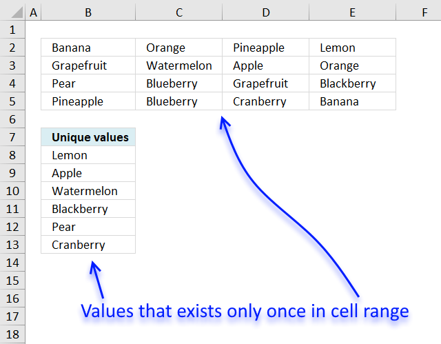
Unique values are values occurring only once in cell range. This is what I am going to demonstrate in this blog post using an array formula.
If you are looking for filtering unique distinct values sorted from A to Z, see this blog post: Extract a unique distinct list sorted from A-Z from range Unique distinct values are all values, however, duplicates are merged into one value. In other words, only one instance of each value.
Excel 365 dynamic array formula in cell B8:
This formula spills values to cell B8 and cells below as far as needed. Here's a breakdown of the formula:
- TOCOL(B2:E5): This is the range of cells from which the unique values will be extracted. The TOCOL function is used to convert the range into a single column. This is necessary to prevent the UNIQUE function to extract unique rows/records instead of unique values.
- UNIQUE(...,,TRUE): This is the function that returns the unique values.
- ,,TRUE: This is an optional argument that specifies whether to return unique values in the order they appear in the original range. The TRUE value means that unique values will be returned, FALSE returns unique distinct values.
Note that if you want to return the unique values in a different order (e.g., sorted), you can use the SORT function in combination with the UNIQUE function.
The following formula is for Excel 2019, array formula in cell B8:
To enter an array formula, type the formula in a cell then press and hold CTRL + SHIFT simultaneously, now press Enter once. Release all keys.
The formula bar now shows the formula with a beginning and ending curly bracket telling you that you entered the formula successfully. Don't enter the curly brackets yourself.
Explaining formula in cell B8
Step 1 - Identify unique values
The COUNTIF function counts values based on a condition or criteria, if number is 1 then value must be unique.
COUNTIF($B$2:$E$5, $B$2:$E$5)=1
becomes
COUNTIF({"Banana", "Orange", "Pineapple", "Lemon";"Grapefruit", "Watermelon", "Apple", "Orange";"Pear", "Blueberry", "Grapefruit", "Blackberry";"Pineapple", "Blueberry", "Cranberry", "Banana"}, {"Banana", "Orange", "Pineapple", "Lemon";"Grapefruit", "Watermelon", "Apple", "Orange";"Pear", "Blueberry", "Grapefruit", "Blackberry";"Pineapple", "Blueberry", "Cranberry", "Banana"})=1
becomes
{2,2,2,1;2,1,1,2;1,2,2,1;2,2,1,2}=1
and returns
{FALSE, FALSE, FALSE, TRUE;FALSE, TRUE, TRUE, FALSE;TRUE, FALSE, FALSE, TRUE;FALSE, FALSE, TRUE, FALSE}.
Step 2 - Keep track of previous values
The first argument in the COUNTIF function contains an expanding cell reference, it grows when the cell is copied to cells below. This makes the formula aware of values displayed in cells above.
COUNTIF(B7:$B$7, $B$2:$E$5)
becomes
COUNTIF("Unique values", {"Banana", "Orange", "Pineapple", "Lemon";"Grapefruit", "Watermelon", "Apple", "Orange";"Pear", "Blueberry", "Grapefruit", "Blackberry";"Pineapple", "Blueberry", "Cranberry", "Banana"})
and returns
{0,0,0,0;0,0,0,0;0,0,0,0;0,0,0,0}.
Step 3 - Add arrays
First we add the arrays and then we check if a number is equal to 1. We then know that the value has not been shown and that it must be unique.
(COUNTIF($B$2:$E$5, $B$2:$E$5)=1)+COUNTIF(B7:$B$7, $B$2:$E$5))=1
becomes
({FALSE, FALSE, FALSE, TRUE;FALSE, TRUE, TRUE, FALSE;TRUE, FALSE, FALSE, TRUE;FALSE, FALSE, TRUE, FALSE}+{0,0,0,0;0,0,0,0;0,0,0,0;0,0,0,0})=1
becomes
{0,0,0,1;0,1,1,0;1,0,0,1;0,0,1,0}=1
and returns
{FALSE, FALSE, FALSE, TRUE;FALSE, TRUE, TRUE, FALSE;TRUE, FALSE, FALSE, TRUE;FALSE, FALSE, TRUE, FALSE}.
Step 4 - Replace TRUE with unique number
The IF function returns unique number if boolean value is TRUE. FALSE returns "" (nothing).
IF(((COUNTIF($B$2:$E$5, $B$2:$E$5)=1)+COUNTIF(B7:$B$7, $B$2:$E$5))=1, (ROW($B$2:$E$5)+(1/(COLUMN($B$2:$E$5)+1)))*1, "")
becomes
IF({FALSE, FALSE, FALSE, TRUE;FALSE, TRUE, TRUE, FALSE;TRUE, FALSE, FALSE, TRUE;FALSE, FALSE, TRUE, FALSE}, (ROW($B$2:$E$5)+(1/(COLUMN($B$2:$E$5)+1)))*1, "")
This part of the formula: (ROW($B$2:$E$5)+(1/(COLUMN($B$2:$E$5)+1)))*1 creates a unique value for each cell in cell range. This makes it easier to extract the correct value in a later step.
IF({FALSE, FALSE, FALSE, TRUE;FALSE, TRUE, TRUE, FALSE;TRUE, FALSE, FALSE, TRUE;FALSE, FALSE, TRUE, FALSE}, (ROW($B$2:$E$5)+(1/(COLUMN($B$2:$E$5)+1)))*1, "")
becomes
IF({FALSE, FALSE, FALSE, TRUE;FALSE, TRUE, TRUE, FALSE;TRUE, FALSE, FALSE, TRUE;FALSE, FALSE, TRUE, FALSE}, {2.33333333333333, 2.25, 2.2, 2.16666666666667;3.33333333333333, 3.25, 3.2, 3.16666666666667;4.33333333333333, 4.25, 4.2, 4.16666666666667;5.33333333333333, 5.25, 5.2, 5.16666666666667}, "")
and returns
{"","","",2.16666666666667;"",3.25,3.2,"";4.33333333333333,"","",4.16666666666667;"","",5.2,""}
Step 5 - Find smallest value in array
The MIN function returns the smallest number in array ignoring blanks and text values.
MIN(IF(((COUNTIF($B$2:$E$5, $B$2:$E$5)=1)+COUNTIF(B7:$B$7, $B$2:$E$5))=1, (ROW($B$2:$E$5)+(1/(COLUMN($B$2:$E$5)+1)))*1, ""))
becomes
MIN({"","","",2.16666666666667;"",3.25,3.2,"";4.33333333333333,"","",4.16666666666667;"","",5.2,""})
and returns 2.16666666666667.
Step 4 - Find corresponding value
IF(MIN(IF(((COUNTIF($B$2:$E$5, $B$2:$E$5)=1)+COUNTIF(B7:$B$7, $B$2:$E$5))=1, (ROW($B$2:$E$5)+(1/(COLUMN($B$2:$E$5)+1)))*1, ""))=(ROW($B$2:$E$5)+(1/(COLUMN($B$2:$E$5)+1)))*1, $B$2:$E$5, "")
becomes
IF(2.16666666666667=(ROW($B$2:$E$5)+(1/(COLUMN($B$2:$E$5)+1)))*1, $B$2:$E$5, "")
becomes
IF(2.16666666666667={2.33333333333333, 2.25, 2.2, 2.16666666666667;3.33333333333333, 3.25, 3.2, 3.16666666666667;4.33333333333333, 4.25, 4.2, 4.16666666666667;5.33333333333333, 5.25, 5.2, 5.16666666666667}, $B$2:$E$5, "")
becomes
IF({FALSE, FALSE, FALSE, TRUE;FALSE, FALSE, FALSE, FALSE;FALSE, FALSE, FALSE, FALSE;FALSE, FALSE, FALSE, FALSE}, $B$2:$E$5, "")
and returns
{"","","","Lemon";"","","","";"","","","";"","","",""}.
Step 5 - Concatenate strings in array
The TEXTJOIN function returns values concatenated ignoring blanks in array.
TEXTJOIN("", TRUE, IF(MIN(IF(((COUNTIF($B$2:$E$5, $B$2:$E$5)=1)+COUNTIF(B7:$B$7, $B$2:$E$5))=1, (ROW($B$2:$E$5)+(1/(COLUMN($B$2:$E$5)+1)))*1, ""))=(ROW($B$2:$E$5)+(1/(COLUMN($B$2:$E$5)+1)))*1, $B$2:$E$5, ""))
becomes
TEXTJOIN("", TRUE, {"","","","Lemon";"","","","";"","","","";"","","",""})
and returns "Lemon" in cell B8.
Filter unique values from a range (for older Excel versions)

Array formula in B10:
copied down as far as necessary.
Named ranges
tbl (B4:E7)
What is named ranges?
How to implement array formula to your workbook
Change the named range. If your list starts at, for example, F3. Change $B$9:B9 in the above formulas to F2:$F$2.
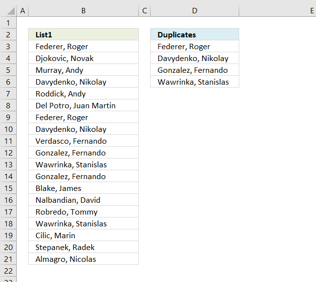
5. Filter unique values sorted from A to Z
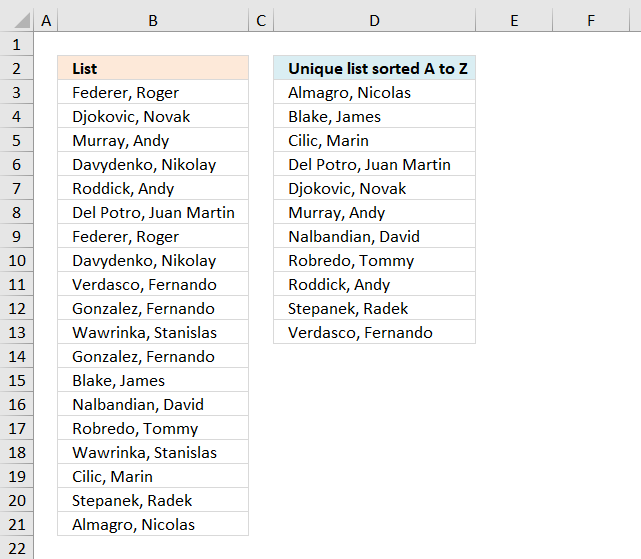
A unique value is a value that only exists once in a list.

A unique distinct list contains all cell values but duplicates are merged into one distinct cell value.

If your are looking for a unique distinct list array formula, see this blog article:
Create a unique distinct alphabetically sorted list
The following array formula extracts unique values from column B in cell D3 and below:
To enter an array formula, type the formula in a cell then press and hold CTRL + SHIFT simultaneously, now press Enter once. Release all keys.
The formula bar now shows the formula with a beginning and ending curly bracket telling you that you entered the formula successfully. Don't enter the curly brackets yourself.
Update 10th December 2020, Excel 365 formula:
This is a regular formula, you can read about it here: Extract unique values sorted from A to Z
Explaining formula in cell D3
Step 1 - Identify unique values
The COUNTIF function counts cells in cell range based on a condition or criteria. If the value is equal to 1 then it must be a unique value.
COUNTIF($B$3:$B$21, $B$3:$B$21)=1
becomes
COUNTIF({"Federer, Roger "; "Djokovic, Novak "; "Murray, Andy "; "Davydenko, Nikolay "; "Roddick, Andy "; "Del Potro, Juan Martin "; "Federer, Roger "; "Davydenko, Nikolay "; "Verdasco, Fernando "; "Gonzalez, Fernando "; "Wawrinka, Stanislas "; "Gonzalez, Fernando "; "Blake, James "; "Nalbandian, David "; "Robredo, Tommy "; "Wawrinka, Stanislas "; "Cilic, Marin "; "Stepanek, Radek "; "Almagro, Nicolas "},{"Federer, Roger "; "Djokovic, Novak "; "Murray, Andy "; "Davydenko, Nikolay "; "Roddick, Andy "; "Del Potro, Juan Martin "; "Federer, Roger "; "Davydenko, Nikolay "; "Verdasco, Fernando "; "Gonzalez, Fernando "; "Wawrinka, Stanislas "; "Gonzalez, Fernando "; "Blake, James "; "Nalbandian, David "; "Robredo, Tommy "; "Wawrinka, Stanislas "; "Cilic, Marin "; "Stepanek, Radek "; "Almagro, Nicolas "})=1
becomes
{2;1;1;2;1;1;2;2;1;2;2;2;1;1;1;2;1;1;1}=1
and returns
{FALSE; TRUE; TRUE; FALSE; TRUE; TRUE; FALSE; FALSE; TRUE; FALSE; FALSE; FALSE; TRUE; TRUE; TRUE; FALSE; TRUE; TRUE; TRUE}
Step 2 - Build an array containing rank if list were sorted
The less than sign concatenated with the cell reference in the second argument in the COUNTIF function makes it return the rank number if list were sorted from A to Z.
COUNTIF($B$3:$B$21,"<"&$B$3:$B$21)
becomes
COUNTIF({"Federer, Roger "; "Djokovic, Novak "; "Murray, Andy "; "Davydenko, Nikolay "; "Roddick, Andy "; "Del Potro, Juan Martin "; "Federer, Roger "; "Davydenko, Nikolay "; "Verdasco, Fernando "; "Gonzalez, Fernando "; "Wawrinka, Stanislas "; "Gonzalez, Fernando "; "Blake, James "; "Nalbandian, David "; "Robredo, Tommy "; "Wawrinka, Stanislas "; "Cilic, Marin "; "Stepanek, Radek "; "Almagro, Nicolas "},"<"&{"Federer, Roger "; "Djokovic, Novak "; "Murray, Andy "; "Davydenko, Nikolay "; "Roddick, Andy "; "Del Potro, Juan Martin "; "Federer, Roger "; "Davydenko, Nikolay "; "Verdasco, Fernando "; "Gonzalez, Fernando "; "Wawrinka, Stanislas "; "Gonzalez, Fernando "; "Blake, James "; "Nalbandian, David "; "Robredo, Tommy "; "Wawrinka, Stanislas "; "Cilic, Marin "; "Stepanek, Radek "; "Almagro, Nicolas "})
becomes
COUNTIF({"Federer, Roger "; "Djokovic, Novak "; "Murray, Andy "; "Davydenko, Nikolay "; "Roddick, Andy "; "Del Potro, Juan Martin "; "Federer, Roger "; "Davydenko, Nikolay "; "Verdasco, Fernando "; "Gonzalez, Fernando "; "Wawrinka, Stanislas "; "Gonzalez, Fernando "; "Blake, James "; "Nalbandian, David "; "Robredo, Tommy "; "Wawrinka, Stanislas "; "Cilic, Marin "; "Stepanek, Radek "; "Almagro, Nicolas "}, {"<Federer, Roger ";"<Djokovic, Novak ";"<Murray, Andy ";"<Davydenko, Nikolay ";"<Roddick, Andy ";"<Del Potro, Juan Martin ";"<Federer, Roger ";"<Davydenko, Nikolay ";"<Verdasco, Fernando ";"<Gonzalez, Fernando ";"<Wawrinka, Stanislas ";"<Gonzalez, Fernando ";"<Blake, James ";"<Nalbandian, David ";"<Robredo, Tommy ";"<Wawrinka, Stanislas ";"<Cilic, Marin ";"<Stepanek, Radek ";"<Almagro, Nicolas "})
and returns
{7; 6; 11; 3; 14; 5; 7; 3; 16; 9; 17; 9; 1; 12; 13; 17; 2; 15; 0}
Step 3 - Replace boolean value TRUE with rank number
The IF function returns one value (argument2) if TRUE and another (argument3) if FALSE.
IF(COUNTIF($B$3:$B$21,$B$3:$B$21)=1,COUNTIF($B$3:$B$21,"<"&$B$3:$B$21),"")
becomes
IF({FALSE; TRUE; TRUE; FALSE; TRUE; TRUE; FALSE; FALSE; TRUE; FALSE; FALSE; FALSE; TRUE; TRUE; TRUE; FALSE; TRUE; TRUE; TRUE},COUNTIF($B$3:$B$21,"<"&$B$3:$B$21),"")
becomes
IF({FALSE; TRUE; TRUE; FALSE; TRUE; TRUE; FALSE; FALSE; TRUE; FALSE; FALSE; FALSE; TRUE; TRUE; TRUE; FALSE; TRUE; TRUE; TRUE}, {7; 6; 11; 3; 14; 5; 7; 3; 16; 9; 17; 9; 1; 12; 13; 17; 2; 15; 0},"")
and returns
{""; 6; 11; ""; 14; 5; ""; ""; 16; ""; ""; ""; 1; 12; 13; ""; 2; 15; 0}.
Step 4 - Extract the smallest value
The SMALL function lets you calculate the k-th smallest value in a cell range or array. SMALL( array, k)
SMALL(IF(COUNTIF($B$3:$B$21, $B$3:$B$21)=1, COUNTIF($B$3:$B$21, "<"&$B$3:$B$21), ""), ROWS(D2:$D$2))
becomes
SMALL({""; 6; 11; ""; 14; 5; ""; ""; 16; ""; ""; ""; 1; 12; 13; ""; 2; 15; 0}, ROWS(D2:$D$2))
The ROWS function in the second argument has an expanding cell reference that grows when cell D3 is copied to cells below. This makes the formula return a new value in each cell except if duplicates exist in the list.
SMALL({""; 6; 11; ""; 14; 5; ""; ""; 16; ""; ""; ""; 1; 12; 13; ""; 2; 15; 0}, ROWS(D2:$D$2))
becomes
SMALL({""; 6; 11; ""; 14; 5; ""; ""; 16; ""; ""; ""; 1; 12; 13; ""; 2; 15; 0}, 1)
and returns 0 (zero).
Step 5 - Get position in array
The MATCH function finds the relative position of a value in an array or cell range.
MATCH(SMALL(IF(COUNTIF($B$3:$B$21, $B$3:$B$21)=1, COUNTIF($B$3:$B$21, "<"&$B$3:$B$21), ""), ROWS(D2:$D$2)), COUNTIF($B$3:$B$21, "<"&$B$3:$B$21), 0)
becomes
MATCH(0, COUNTIF($B$3:$B$21, "<"&$B$3:$B$21), 0)
becomes
MATCH(0, {7; 6; 11; 3; 14; 5; 7; 3; 16; 9; 17; 9; 1; 12; 13; 17; 2; 15; 0}, 0)
and returns 19.
Step 6 - Return value
The INDEX function returns a value based on row number (and column number if needed)
INDEX($B$3:$B$21, MATCH(SMALL(IF(COUNTIF($B$3:$B$21, $B$3:$B$21)=1, COUNTIF($B$3:$B$21, "<"&$B$3:$B$21), ""), ROWS(D2:$D$2)), COUNTIF($B$3:$B$21, "<"&$B$3:$B$21), 0))
becomes
INDEX($B$3:$B$21, 19)
and returns "Almagro, Nicolas " in cell D3.
Get Excel *.xlsx file
Extract-a-unique-list sorted A to Z from a column-in-excel.xlsx
6. Find min and max unique and duplicate numerical values
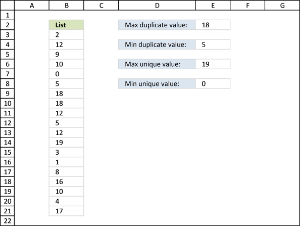
Table of Contents
- How to find the largest duplicate number
- How to find the largest duplicate number - Excel 365
- How to find the smallest duplicate number
- How to find the smallest duplicate number - Excel 365
- How to find the largest unique number
- How to find the largest unique number - Excel 365
- How to find the smallest unique number
- How to find the smallest unique number - Excel 365
- Get Excel *.xlsx file
6.1. Extract the largest duplicate number
Question: How do I get the largest and smallest unique and duplicate value?
The image below shows you a list of numbers in column B ($B$3:$B$21).
Max duplicate value, array formula in E2:
The largest number in the list above is 19 but it is a unique number meaning it exists only once. Number 18 is the largest duplicate number, 18 is in cell B9 and B10.
To enter an array formula, type the formula in a cell then press and hold CTRL + SHIFT simultaneously, now press Enter once. Release all keys.
The formula bar now shows the formula with a beginning and ending curly bracket telling you that you entered the formula successfully. Don't enter the curly brackets yourself.
6.1.1 Explaining formula in cell E2
Step 1 - Count the frequency of each value
The COUNTIF function counts values based on a condition or criteria, in this case, it counts all values in the cell range.
COUNTIF($B$3:$B$21,$B$3:$B$21)
returns {1; 3; 1; ... ; 1}.
Step 2 - Extract duplicate numbers
The IF function returns the row number if cell is a duplicate. FALSE returns "" (nothing).
IF(COUNTIF($B$3:$B$21,$B$3:$B$21)>1,$B$3:$B$21,)
returns {0; 12; 0; ... ; 0}.
Step 3 - Return largest value
The MAX function returns the maximum value from a cell range or array.
MAX(IF(COUNTIF($B$3:$B$21,$B$3:$B$21)>1,$B$3:$B$21,))
becomes
MAX({0; 12; 0; 10; 0; 5; 18; 18; 12; 5; 12; 0; 0; 0; 0; 0; 10; 0; 0})
and returns 18 in cell E2.
6.2. Extract the largest duplicate number - Excel 365

Formula in cell D3:
6.2.1 Explaining formula
Step 1 - Count each item
The COUNTIF function calculates the number of cells that meet a given condition.
COUNTIF(range, criteria)
COUNTIF($B$3:$B$21, $B$3:$B$21)
returns
{1; 3; 1; 2; 1; 2; 2; 2; 3; 2; 3; 1; 1; 1; 1; 1; 2; 1; 1}.
Step 2 - Check if larger than one meaning it is a duplicate
The larger than sign is a logical operator that lets you find numbers larger than a given condition. In this case, if larger than one means it is a duplicate.
COUNTIF($B$3:$B$21,$B$3:$B$21)>1
becomes
{1; 3; 1; ... ; 1}>1
and returns
{FALSE; TRUE; ... ; FALSE}
Step 3 - Filter duplicates
The FILTER function lets you extract values/rows based on a condition or criteria.
FILTER(array, include, [if_empty])
FILTER(B3:B21, COUNTIF($B$3:$B$21, $B$3:$B$21)>1)
becomes
FILTER({2; 12; 9; ... ; 17}, {FALSE; TRUE; FALSE; ... ; FALSE})
and returns
{12; 10; ... ; 10}.
Step 4 - Get largest value
The MAX function gets the largest number in a cell range or array.
MAX(number1, [number2], ...)
MAX(FILTER(B3:B21,COUNTIF($B$3:$B$21,$B$3:$B$21)>1))
becomes
MAX({12; 10; 5; 18; 18; 12; 5; 12; 10})
and returns 18.
6.3. Extract the smallest duplicate number

Formula in cell
The smallest number in the list above is 0 but it is a unique number meaning it exists only once. Number 5 is the smallest duplicate number, 18 is in cell B8 and B12.
This formula is almost identical to the formula in section 1, only MAX function is replaced with the MIN function. See the formula explanation above in section 1.
6.4. Extract the smallest duplicate number - Excel 365

Formula in cell D3:
This formula is almost identical to the formula in section 2, only the MAX function is replaced with the MIN function. See the formula explanation above in section 2.
6.5. Extract the largest unique number

Max unique value, formula in D3:
The largest unique number in the list above is 19.
6.5.1 Explaining formula
Step 1 - Count values
The COUNTIF function calculates the number of cells that meet a given condition.
COUNTIF(range, criteria)
COUNTIF($B$3:$B$21, $B$3:$B$21)
becomes
COUNTIF({2; 12; 9; ... ; 17}, {2; 12; 9; ... ; 17})
and returns
{1; 3; 1; ... ; 1}.
Step 2 - Check if a number is one
A value equal to one must be a unique value, it exists only once. The equal sign is a logical operator that lets you compare values in an Excel formula.
COUNTIF($B$3:$B$21, $B$3:$B$21)=1
returns {TRUE; FALSE; ... ; TRUE}.
Step 3 - Evaluate IF function
IF(COUNTIF($B$3:$B$21, $B$3:$B$21)=1, $B$3:$B$21, )
becomes
IF({TRUE; FALSE; TRUE; ... ; TRUE}, {2; 12; 9; ... ; 17}, )
and returns
{2; 0; ... ; 17}.
Step 4 - Get the largest number in the array
The MAX function gets the largest number in a cell range or array.
MAX(number1, [number2], ...)
MAX(IF(COUNTIF($B$3:$B$21, $B$3:$B$21)=1, $B$3:$B$21, ))
becomes
MAX({2; ... ; 19; ... ; 17})
and returns 19.
6.6. Extract the largest unique number - Excel 365

Formula in cell D3:
Explaining formula
Step 1 - Extract unique numbers in cell range B3:B21
The UNIQUE function lets you extract both unique and unique distinct values.
UNIQUE(array, [by_col], [exactly_once])
UNIQUE(B3:B21, , TRUE)
becomes
UNIQUE({2; 12; 9; ... ; 17}, , TRUE)
and returns
{2; 9; ... ; 17}
Step 2 - Get largest number in array
The MAX function gets the largest number in a cell range or array.
MAX(number1, [number2], ...)
MAX(UNIQUE(B3:B21, , TRUE))
becomes
MAX({2; 9; 0; 19; ... ; 17})
and returns 19.
6.7. Extract the smallest unique number

Min unique value, formula in E8:
The smallest unique number in the list above is 0.
This formula is almost identical to the formula in section 5, only the MAX function is replaced with the MIN function. See the formula explanation above in section 5.
6.8. Extract the smallest unique number - Excel 365

Excel 365 dynamic array formula in cell D3:
This formula is almost identical to the formula in section 6, only the MAX function is replaced with the MIN function. See the formula explanation above in section 6.
6.9 Get Excel *.xlsx file
7. Filter unique strings from a cell range

This section describes how to create a list of unique words from a cell range. Unique words are all words that exist once in a given cell range.
Cell range B3:B15 contains values, see picture above.
What's on this section
7.1. Filter unique strings in a range - UDF

Rick Rothstein (MVP - Excel) helped me out here with a powerful user defined function (udf).
Array formula in cell B2:B23
This is how you enter an array formula, type the formula in a cell then press and hold CTRL + SHIFT simultaneously, now press Enter once. Release all keys.
The formula bar now shows the formula with a beginning and ending curly bracket telling you that you entered the formula successfully. Don't enter the curly brackets yourself.
Array formula in cell C2:C23
Select all the cells to be filled, then type the above formula into the Formula Bar and press CTRL+SHIFT+ENTER
User defined function

Instructions
- You can select far more cells to load the formulas in than are required by the list. The empty text string will be displayed for cells not having an entry.
- You can specify a larger range than the there are filled in cells as the argument to these macros to allow for future entries in the column.
- You can specify whether the listing is to be case sensitive or not via the optional second argument with the default value being FALSE, meaning duplicated entries with different casing like One, one, ONE, onE, etc.. will all be treated as if they were the same word with the same spelling. If you pass TRUE for that optional second argument, then those words would all be treated as if they were different words.
- For all the "Case Insensitive" listing, the words are listed in Proper Case (first letter upper case, remaining letters lower case). The reason being if you had One, one and ONE then there is not reason to prefer one version over another, so I solved the problem by using Proper Case throughout.
VBA Code:
Function UniqueWords(Rng As Range, Optional  CaseSensitive As Boolean) As Variant
Dim X As Long, WordCount As Long,  List As String, Uniques As Variant, Words() As String
List =  WorksheetFunction.Trim(Replace(Join(WorksheetFunction.Transpose(Rng)), Chr(160),  " "))
Words = Split(List)
For X = 0 To  UBound(Words)
If CaseSensitive  Then
If UBound(Split(" " &; List & " ",  " " & Words(X) & " ")) = 1  Then
Uniques = Uniques &  Words(X) & " "
List =  Replace(List, Words(X), "")
End  If
Else
If  UBound(Split(" " & UCase(List) & " ", " " & UCase(Words(X)) & "  ")) = 1 Then
Uniques = Uniques  & StrConv(Words(X), vbProperCase) & "  "
List = Replace(List, Words(X),  "")
End If
End  If
Next
Uniques = WorksheetFunction.Trim(Uniques)
Words = Split(Uniques)
If Application.Caller.Count > UBound(Words)  Then
Uniques = Uniques & Space(Application.Caller.Count - UBound(Words))
End If
UniqueWords = WorksheetFunction.Transpose(Split(Uniques))
End  Function
How to implement user defined function in excel
- Press Alt-F11 to open visual basic editor
- Press with left mouse button on Module on the Insert menu
- Copy and paste the above user defined function
- Exit visual basic editor
- Select a sheet
- Select a cell range
- Type =UniqueWords($A$2:$A$18, TRUE) into formula bar and press CTRL+SHIFT+ENTER
Get Rick Rothstein's Excel example file
Many thanks to Rick Rothstein (Mvp - Excel)!!
7.2. Filter unique strings in a range - Excel 365
The image above demonstrates a formula in cell D3 that extracts unique strings based on the space character as a delimiting character. A unique string is a string that exists only once in a cell range.
Note, string "Us" is equal to "US", in other words, this is not a case-sensitive formula.
Excel 365 formula in cell D3:
Explaining formula
Step 1 - Join cell values
The TEXTJOIN function combines text strings from multiple cell ranges and also use delimiting characters if you want.
TEXTJOIN(delimiter, ignore_empty, text1, [text2], ...)
TEXTJOIN(" ", TRUE, B3:B15)
returns
"3M - Asia 3M South America 3M - Africa 3M - US 3M - ASIA 3M - Us 3M - South AMERICA 3M - Europe 3M Australia 3M Australia 3M Europe 3M aSIA 3M US".
Step 2 - Split strings based on space as a delimiting character
The TEXTSPLIT function splits a string into an array across columns and rows based on delimiting characters.
TEXTSPLIT(Input_Text, col_delimiter, [row_delimiter], [Ignore_Empty])
TEXTSPLIT(TEXTJOIN(" ", TRUE, B3:B15), , " ", TRUE, 0)
returns {"3M"; "-"; "Asia"; ... ; "US"}.
Step 3 - List unique strings
The UNIQUE function extracts both unique and unique distinct values and also compare columns to columns or rows to rows.
UNIQUE(array,[by_col],[exactly_once])
UNIQUE(TEXTSPLIT(TEXTJOIN(" ", TRUE, B3:B15), , " ", TRUE, 0), , TRUE)
returns "Africa".
8. How to extract a case sensitive unique list from a column
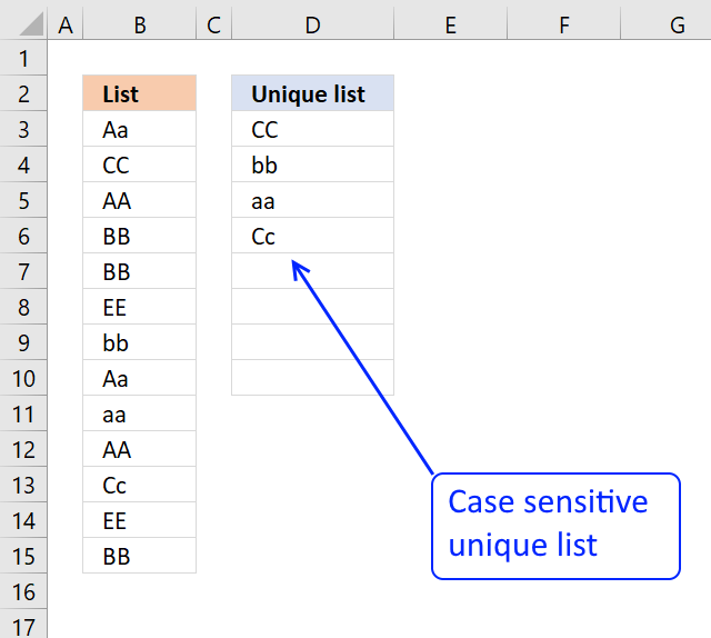
This section demonstrates a formula that extracts unique values from a column also considering upper and lower characters (case sensitive).
My definition of unique values is values that exist only once in a cell range. The image below shows you a list in column B, some of these values have duplicates.
The list in column D contains only values that are unique, Aa and BB exist only once in the list, all other values have a duplicate.
The formula extracts CC, bb, aa and Cc because they exist only once in column B.
Array formula in cell D3:
If you are looking for a unique distinct list, read this post: Extract unique distinct values (case sensitive) [Formula].
This post explains how to do a case-sensitive VLOOKUP and returning multiple values:
Recommended articles
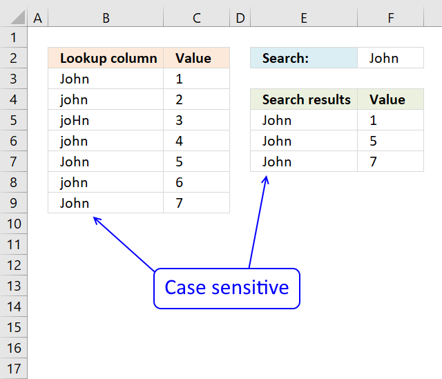
The array formula in cell F5 returns adjacent values from column C where values in column B matches the search […]
Make sure you read the following article if you want to extract duplicate values:
Recommended articles
The array formula in cell C2 extracts duplicate values from column A. Only one duplicate of each value is displayed […]
8.1 How to enter an array formula
- Copy (Ctrl + c) above formula.
- Double press with left mouse button on cell C2.
- Paste (Ctrl + v) to cell C2.
- Press and hold CTRL + SHIFT simultaneously.
- Press Enter once.
- Release all keys.
Your formula now looks like this: {=array_formula}
Don't enter the curly brackets, they appear automatically.
Recommended articles

Array formulas allows you to do advanced calculations not possible with regular formulas.
8.2 Explaining array formula in cell D3:
You can easily follow along if you get the attached file and select cell D3. Then go to tab "Formulas" on the ribbon and press with left mouse button on the "Evaluate Formula" button.
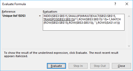
Press with left mouse button on "Evaluate" button shown in above picture to move to next step.
Step 1 - Check if values are case sensitive
The EXACT function is case sensitive function that allows you to compare values. If they match EXACT returns TRUE, if not FALSE.
EXACT($B$3:$B$15,TRANSPOSE(B$3:$B$15))*1
If we use TRANSPOSE we can compare values against each other to build an array, in a single calculation. The following picture shows you this array as an index table, I have highlighted cells that match green. Example, cell C3 shows you the result of a comparison between the value in cell C2 and B3. Since it is the same value they must match and the formula returns 1 and is highlighted green.
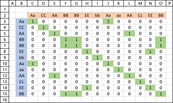
It is now obvious that value Aa has a duplicate because cell J3 is also highlighted green.
Incredible that Excel allows you to do such a complicated calculation in a single cell.
Step 2 - MMULT function lets you SUM values column-wise or row-wise
The MMULT function is like the SUMPRODUCT function but on steroids, let me explain. SUMPRODUCT lets you multiply and then sum values, the result is a single value.
MMULT lets you multiply and sum values either column-wise or row-wise, the result is an array.
MMULT(EXACT($B$3:$B$15, TRANSPOSE(B$3:$B$15))*1, ROW($B$3:$B$15)^0) is entered in column P, see picture below.
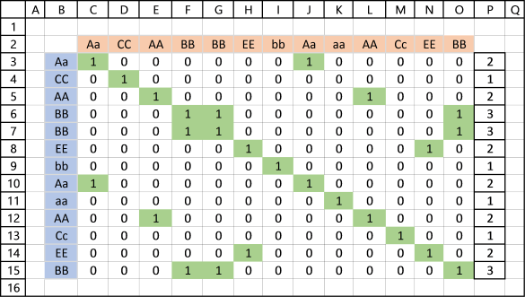
It is now easy to spot unique values in the index table, if column P contains 1 the corresponding value in column B must be unique.
Step 3 - Check if value in array is equal to 1 and if so return corresponding row number
Column Q shows you corresponding relative row number if value in column P is equal to 1.
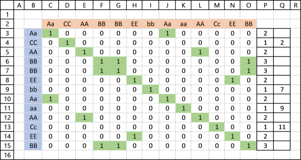
IF(MMULT(EXACT($B$3:$B$15, TRANSPOSE(B$3:$B$15))*1, ROW($B$3:$B$15)^0)=1, MATCH(ROW($B$3:$B$15), ROW($B$3:$B$15)), "")
returns this array: {"";2;"";""; "";"";7; "";9;"";11; "";""}
Step 4 - Filter the k-th smallest row number
SMALL(IF(MMULT(EXACT($B$3:$B$15, TRANSPOSE(B$3:$B$15))*1, ROW($B$3:$B$15)^0)=1, MATCH(ROW($B$3:$B$15), ROW($B$3:$B$15)), ""),ROWS($A$1:A1))
becomes SMALL({"";2;"";""; "";"";7; "";9;"";11; "";""},1) and returns 2.
Step 5 - Return value based on coordinate
INDEX($B$3:$B$15, SMALL(IF(MMULT(EXACT($B$3:$B$15, TRANSPOSE(B$3:$B$15))*1, ROW($B$3:$B$15)^0)=1, MATCH(ROW($B$3:$B$15), ROW($B$3:$B$15)), ""),ROWS($A$1:A1)))
becomes INDEX($B$3:$B$15, 2) returns "CC" in cell D3.
9. Extract a case sensitive unique list from a column - Excel 365

Formula in cell D3:
The following formula is for Excel 365 users:
9.1 Explaining formula
Step 1 - Convert a vertical array to horizontal
The TRANSPOSE function allows you to convert a vertical range to a horizontal range, or vice versa. This works also with arrays.
TRANSPOSE(B3:B15)
returns {"Aa", "CC", ... , "BB"}
Step 2 - Check if values match (case sensitive)
The EXACT function allows you to check if two values are precisely the same, it returns TRUE or FALSE. The EXACT function also considers upper and lower case letters.
EXACT(B3:B15, TRANSPOSE(B3:B15))
returns the following array displayed in the image below.

The image above shows the array in cell range C3:O15. It compares each value against each other and if there are two or more TRUE the value has a duplicate.
Step 3 - Multiply with 1
The MMULT function can't work with boolean values (TRUE or FALSE) , however, there is a workaround. They have numerical equivalents that work with the MMULT function.
TRUE = 1
FALSE = 0 (zero)
EXACT(B3:B15, TRANSPOSE(B3:B15))*1
returns the following array displayed in the image below.
Step 4 - Create a sequence of 1
The ROW function returns a number representing a row number based on a cell reference. If the cell reference points to multiple cells an array of numbers is returned.
ROW(B3:B15)^0
becomes
{3; 4; ... ; 15}^0
and returns {1; ... ; 1}.
Step 5 - Sum values row-wise
The MMULT function calculates the matrix product of two arrays, this can be used to sum values either column-wise or row-wise, the result is an array.
MMULT(EXACT(B3:B15, TRANSPOSE(B3:B15))*1, ROW(B3:B15)^0)
returns the following array displayed in the image below in column P.
The image above shows the array in column P.
Step 6 - Check if unique
Values that return 1 exist only once, two or more means duplicates.
MMULT(EXACT(B3:B15, TRANSPOSE(B3:B15))*1, ROW(B3:B15)^0)=1
and returns {FALSE; TRUE; ... ; FALSE}.
Step 7 - Filter unique values
The FILTER function lets you extract values/rows based on a condition or criteria.
FILTER(B3:B15, MMULT(EXACT(B3:B15, TRANSPOSE(B3:B15))*1, ROW(B3:B15)^0)=1)
returns {"CC"; "bb"; "aa"; "Cc"}.
Step 8 - Shorten formula
The LET function assigns names to calculation results. This can shorten formulas considerably and make them run much faster.
LET(name1, name_value1, calculation_or_name2, [name_value2, calculation_or_name3...])
LET(z, B3:B15, FILTER(z, MMULT(EXACT(z, TRANSPOSE(z))*1, ROW(z)^0)=1))
Unique values category

First, let me explain the difference between unique values and unique distinct values, it is important you know the difference […]
Excel categories
37 Responses to “Working with unique values”
Leave a Reply
How to comment
How to add a formula to your comment
<code>Insert your formula here.</code>
Convert less than and larger than signs
Use html character entities instead of less than and larger than signs.
< becomes < and > becomes >
How to add VBA code to your comment
[vb 1="vbnet" language=","]
Put your VBA code here.
[/vb]
How to add a picture to your comment:
Upload picture to postimage.org or imgur
Paste image link to your comment.
Hi,
I've been searching for articles to help me to identify unique data across multiple Excel columns, and yours is the closest I have found. However, it seems to deal with only two (2) columns at a time. Is it expandable to cover more than two, in particular where the columns are not adjacent?
What I have is a grid of results:
Cols A, B, C reference result set 1 (with the potentially duplicate data in Col C)
Cols D, E, F reference result set 2 (with the potentially duplicate data in Col F)
and so on, with potentially result sets. The pracical number of rows involved is likely to be no more than 500.
What I need to do is to count all the unique entries in Col C, Col D, Col as a combined set, such that if Col C has data "abc", and Col also has the same data, then the data is only counted once. (I don't actually need to generate a new list of the unique data, but if that is a required stage in the calculation it is not a problem.) Note that can be any value, but is likely to not exceed 500 columns.
Could you advise me if there is a specific, formulaic (not VBA) solution to the problem? If so, could you provide a clue to solving it?
Many Thanks,
Nigel Edwards.
Thanks for commenting!
Interesting question, I have to think about this question for a while...
I created an array formula that counts unique distinct values in three different ranges.
https://www.get-digital-help.com/count-unique-distinct-values-in-three-columns-combined-in-excel/
Hi Oscar,
Would be possible to share this formula again.
It looks like link is years old and was probably disabled.
Much appreciate.
hi, i'm curious on this solution.
Is there a simpler/shorter formula to extract non-duplicate entries?
output shall be BB and EE (non-duplicates on both columns).
I have updated this blog post. I think the formula is somewhat shorter and uses less named ranges.
xcellent!!! thanks!!
Hi,
Just found the site and wow! I've already fixed a few sloppy problems in some my work spreadsheets.
Sorry in advance if this is the wrong way to ask a question.
But this page is the closet I've found to what I am trying to do. I have a table with four columns, Date, Name, Level, and outcome. The range is from row 3 to row 1000.
What I need to be able to do is look at today's date. Determine the month and year and then look up all the values in the date column that match the month and year. I've been trying to get it to work with sumproduct but I can't wrap my head around it.
Then on a separate tab list all the unique events for that month.
So one the seperate tab it would show something like this:
May 2/2010 Bob Smith 3 Requires Attention
May 5/2010 Jim Smith 1 Out of Service
Hope you are able to help. Thanks in advance.
Dave,
see this post: https://www.get-digital-help.com/list-all-the-unique-events-for-a-month-in-excel-array-formula/
Thanks! Works like a treat
I tried this and it gives a divide by zero error. The reason is countif() gives a 0. What are you trying to do with the countif, seems like that using 2 ranges are arguments is not allowed.
Scott,
I think you might have blanks in your two lists?
Get the Excel file
Scott.xls
I am trying to filter dates (with days) using month and year as follows:
=SUMIFS('DATA INPUT'!$C$3:$C$5000,TEXT('DATA INPUT'!$B$3:$B$5000, "yyyy-mmm"),TEXT(E$1,"yyyy-mmm"),'DATA INPUT'!$D$3:$D$5000,"Pilsner",'DATA INPUT'!$E$3:$E$5000,"Beer pack")
- Column "C" is what I would like to sum
- Column "B" is the dates I am TRYING to filter using E1 (inputted month)
- Column "D" and "E" are standard text to be filtered
I have tried playing with the concepts above but to no avail, any ideas? I would like to avoid VBA, etc.
Chris,
Array formula in F1:
Your formula:
becomes
Entered as an array formula.
I may be a bimbo, but I can't figure this out. I have five rows that need to change, sorted by date from the first row.
here are my row names: due date, author, title, changes, date completed
I want the due dates to all be in order, changing the corresponding columns.
HELP a homegirl out! PLEASE!
oh and i have a MAC.
amber,
Is this what you had in mind?
Sort from left to right
How to find Min and Max numeric values in a range of cells that have duplicate numbers and blanks, but only want to find the Min and Max on the largest/top 100 non-duplicate values.
Marc,
read post:
Find max unique value from a range that have duplicate numbers and blanks
[...] Excel, Search/Lookup, Sort values, table on Nov.20, 2012. Email This article to a Friend Marc asks:How to find Min and Max numeric values in a range of cells that have duplicate numbers and blanks, [...]
Hi
I've gotten this to partially work. The problem is my data is split over 4+ columns. So Column A would be Columns S,AA,AI,etc and column B is Columns O,W,AE,etc.
This works:
Date (S2:S21)
Values (O2:O21)
But when I try to add other columns to the named ranges it doesn't like it. This doesn't work:
Data (S3:S42,AA3:AA24)
Values (O3:O42,W3:W24)
Thanks
Laura,
you are right, it does not work. I don´t have a solution for you.
This formula breaks if you change the size of the "tbl" range to only one or two columns of the same data in the "tbl" range.
How is this fixed so that I could use a range of any size in place of the "tbl" range?
tyler,
the formula works if you use two or more columns. I tried with two columns and it worked.
Use this formula if you are working with one column:
How to extract unique values from a column
Remember, the formulas above filter unique values. If you are looking for unique distinct values, see this post:
Extract a unique distinct list sorted from A-Z from range
Suppose if i want the unique list to be start from F3 means, then i have to change C9:$C$9 to F2:$F$2....but i want the list to be start from F1 then what should i write in the formula...instead of C9:$C$9 can i write F0:$F$0. Note: I dont want any heading. I want the list to be start from F1.Please provide the solution
Shariff,
Suppose if i want the unique list to be start from F3 means, then i have to change C9:$C$9 to F2:$F$2...
Yes, correct!
but i want the list to be start from F1 then what should i write in the formula...instead of C9:$C$9 can i write F0:$F$0. Note: I dont want any heading. I want the list to be start from F1.Please provide the solution
Great question and I don´t know the answer. I don´t think you can.
[…] Excel udf: Filter unique distinct values (case sensitive) […]
error have a problem why does it give the answer "00/01/00"
I tried your formula, it came up with (") in the cell.
What could I have done wrong? Here is the formula.
=ArrayFormula(textjoin("",true,if(min(if(((countif($B$5:$EC$16,$B$5:$EC$16)=1)+countif(A36:$A$36,$B$5:$EC$16))=1,(row($B$5:$EC$16)+(1/(column($B$5:$EC$16)+1)))*1,""))=(row($B$5:$EC$16)+(1/(column($B$5:$EC$16)+1)))*1,$B$5:$EC$16,"")))
RANGE : b5:EC16
output header: A36
Regards
Sunny
Sunny Dhillon,
Try this array formula:
=TEXTJOIN("", TRUE, IF(MIN(IF(((COUNTIF($B$5:$EC$16, $B$5:$EC$16)=1)+COUNTIF(A36:$A$36, $B$5:$EC$16))=1, (ROW($B$5:$EC$16)+(1/(COLUMN($B$5:$EC$16)+1)))*1, ""))=(ROW($B$5:$EC$16)+(1/(COLUMN($B$5:$EC$16)+1)))*1, $B$5:$EC$16, ""))
How to just list out the unique from list 1
Nguyen Hai Tuan
Read this:
https://www.get-digital-help.com/how-to-extract-a-unique-list-and-the-duplicates-in-excel-from-one-column/
Dear Sir,
I handle bankruptcy cases for many companies. The details of each company are maintained in different workbooks. The reporting compliances and the processes have very stringent timelines. I need to have all the details of reporting requirements and processes due yesterday to three days from now on a single master sheet distinct from these workbooks.
The details of the reporting required and processes are on the columns G, I K, M O, R of worksheet "REPORTING" and column h of "PROCESS".
PLEASE help me with a formula or a vba code by which I can get the complete rows where the relevant dates appear on the master sheet mentioned above.
I have tried working with the formulas given by you, as I find your solutions to be effective as you explain them nicely and the logic once clearly understood, can be applied anywhere.
I have been able to get the answer for a column but not the complete row, if I am using the same worksheet or even the same workbook but not on a separate workbook. Besides, I get a #num wherever the dates are out of range. Is it possible to get a blank instead of this error message.
I have been struggling with this for long. Kindly help. I have attched the link to my google drive in the column for website. Just for information I use macbook pro and ms excel for mac.
A big thank you for bringing me upto this point ans bigger thank you in advance for leading me to the destination.
I am trying to count the number of unique strings of characters separated by deliminator in a single cell. The strings are made up of either several numbers, combined numbers and text, or single digit numbers. I need to count:
1- Unique strings of numbers only
2- total sets of strings in a cell
3- total number of single digits
4- total number of unique single digits in a cell
5- total number of words in a cell
6- total number of unique words in a cell (specific words)
Can anyone help me? I've been trying to find answers to this for days now. I was able to find a way to count unique words, but for some reason it doesn't always work. Right now, I'm pressed to find out how to count the unique serial numbers in a cell.
I'm looking to get a count of unique strings of numbers or numbers and text within a single cell, each separated by the vertical bar.
I have searched for days and cannot find anyone that can help me. Surely, you must know how to do this! Please!
MARGIE CHAPPELL
I recommend that you check out the "Text to Columns" feature, it will separate values in a cell separated by a delimiting character into multiple cells.
https://www.laptopmag.com/articles/use-text-columns-excel
Once you have values separated you can use the UDFs I have on my website.
Can this formula be changed to an array formula? I also need the DISTINCT values (not UNIQUE values) from both the columns. for e.g. A,B,C from List 1 and C,D,E from List 2, which when combined should result in A,B,C,D,E.