How to use the INDEX function
What is the INDEX function?
The INDEX function returns a value from a specific position in a cell range, Excel table, or an array based on a row and column number. In my opinion this function is one of the most useful functions in Excel. There are two ways to use the INDEX function: array form or reference form.
What is the difference between the INDEX function and the OFFSET function?
The OFFSET function is also able to extract a 2D range from a given cell range which the INDEX function can't as far as I know.

However, the OFFSET function is volatile meaning it recalculates more often than non-volatile functions. Your Excel worksheet could become significantly slower if you use the OFFSET function frequently.
I recommend using the INDEX function over the OFFSET function as much as possible because of this disadvantage.
Table of Contents
- Introduction
- Syntax
- Example
- Create array constants
- How to get a value in a given cell range based on a row number
- How to return all values in a row or column in a given cell range
- Get a value in a given cell range based on a row and column number
- How to use the [area_num] argument
- How to return the entire row in a given cell range
- How to build a dynamic cell reference
- Function error
- Can you replace the VLOOKUP function with the INDEX function?
- Where do I use the INDEX - MATCH functions instead of VLOOKUP?
- Get Excel file
- Get the latest revision
- Create a list with most recent data available
1. Introduction
What if you compare the new Excel 365 FILTER function with the INDEX function?
The new FILTER function lets you create much smaller formulas and is really powerful. It replaces the INDEX function in lots of situations. Check out the FILTER function examples.
Can the INDEX function return multiple values?
Yes, it can. Excel versions earlier than Excel 365 need to enter the formula as an array formula for it to work. This is what the INDEX function can do:
- Return all values in a given row or column. See section 6, section 9.1 and 9.2
- Return all values in a given cell range. See section 8.
- A formula that return a single value, however, the formula is constructed so it returns a new value in each cell. This technique is now more or less obsolete because of the new FILTER function and other new Excel 365 functions.
What is the difference between the INDEX function and the VLOOKUP function?
The INDEX function and the VLOOKUP function are both used to look up values in a table or a range of cells, but they have some differences.
The VLOOKUP function looks up a value in the first column of a range and returns a value from another column in the same row. The column number is specified by a number argument.
For example, =VLOOKUP(A2,B2:D10,3,FALSE) will look up the value in A2 in the first column of B2:D10 and return the value from the third column (column D) in the same row.
The INDEX function returns a value from a specific row and column in a range. The row and column numbers are specified by separate arguments.
For example, =INDEX(B2:D10,4,2) will return the value from the fourth row and second column (cell C5) in the range B2:D10.
One advantage of the INDEX function over the VLOOKUP function is that it can look up values in any column of a range, not just the first one. Another advantage of the VLOOKUP function over the INDEX function is that it is simpler to use and learn and requires fewer arguments, however, the INDEX and MATCH functions are more versatile.
1. Syntax
Array form
INDEX(array, [row_num], [column_num])
Reference form
INDEX(array, [row_num], [column_num], [area_num])
2. Arguments
Array form
| array | Required. The cell range you want to get a value from. You can also use an array. |
| [row_num] | Optional. The relative row number of a specific value you want to get. If omitted the INDEX function returns all values if you enter it as an array formula. Update! The 365 subscription version of Excel returns all values without needing to enter the formulas an array formula. |
| [column_num] | Optional. The relative column number of a specific value you want to get. If omitted the INDEX function returns all values if you enter it as an array formula. Update! The 365 subscription version of Excel returns all values without needing to enter the formulas an array formula. |
| [area_num] | Optional. A number representing the relative position of one of the ranges in the first argument. |
Reference form
| cell reference | Required. A reference a cell range or multiple cell ranges. |
| [row_num] | Optional. The relative row number of a specific value you want to get. If omitted the INDEX function returns all values if you enter it as an array formula. Update! The 365 subscription version of Excel returns all values without needing to enter the formulas an array formula. |
| [column_num] | Optional. The relative column number of a specific value you want to get. If omitted the INDEX function returns all values if you enter it as an array formula. Update! The 365 subscription version of Excel returns all values without needing to enter the formulas an array formula. |
| [area_num] | Optional. A number representing the relative position of one of the ranges in the first argument. |
What is the difference between the array form and the reference form?
The difference between the array form and the reference form of the INDEX function is that the reference form allows more than one array, you also need to use optional argument [area_num] to specify which array should be used.
The array form only allows one array or range as the first argument, however, this is how the INDEX function is most used.. Both forms return a value or a reference based on a given row and column location.
Use the reference form when you have multiple ranges and you want to switch between them based on a condition. Read this section on how to use the reference form:
How to use the [area_num] argument - INDEX function
3. Example
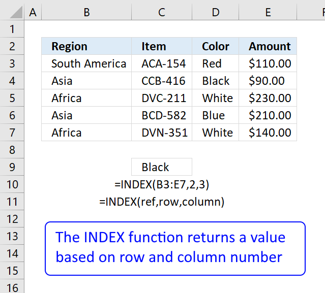
Formula in cell C9:
This formula returns a value from row 2 and column 3 based on cell range B3:E7, note these are relative positions.

The image above shows the relative row and column numbers, row 2 and column 3 are highlighted. The intersection of those two is the value the INDEX function returns.
4. How to create array constants
The first argument in the INDEX function is array or a cell reference to a cell range. What is an array constant? An array constant is a set of values hardcoded into the formula.
To demonstrate in greater detail what an array of constants is you can convert a cell reference to an array of constants:
- Select the cell reference.
- Press F9 to convert the cell reference to values, see the animated image above.
B6:D8
becomes
{"Staple",10,10;"Binder",20,6;"Pen",30,1}
and each value is separated by a delimiting character. Comma (,) is used to separate columns and semicolon (;) to separate rows.
The English language version of excel uses commas and semicolons, other language versions of excel may use other characters. You can change this in the Regional settings in Windows.
Here is an example of array constants used in an INDEX function:
The greatest disadvantage of using an array is that you need to edit the formula if you need to change one of the values in the array, contrary to a cell reference.
Here is an example of a cell reference being used in an INDEX function:
You don't need to edit this formula if one of the values in cell range B6:D8 is changed, the formula is using the new value automatically.
Remember that relative cell references (B6:D8) changes when you copy the cell and paste to cells below. Absolute cell references ($B$6:$D$8) do not change when the cell is copied to cells below.
Read more about converting cell references or formulas:
Replace a formula with its result
5. How to get a value in a given cell range based on a row number
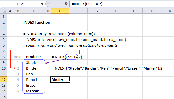
The second argument in the INDEX function is the row_num which you are required to enter, the [column_num] argument is optional however hence the brackets. It allows you to choose the row in an array or cell range, from which to return a value.
If you use an array or cell range with values distributed in one column only there is no need to use the second optional argument which specifies the column, there is only one column to use. Here is an example of an array containing values in a single column, no comma as a delimiting value in this array which would have indicated that there would have been multiple columns.
The following formula uses a cell reference instead of hardcoded values:
Cell range C9:C14 has values separated by a semicolon. The cell range is one-dimensional. In this example, the value from the second row will be returned, see image above.
6. How to return all values in a row or column in a given cell range

It is also possible to return an array of values if you omit or use a zero as row_num argument:
Both these formulas return an array of values. To be able to display all values you need to enter the formula as an array formula in a cell range that has the same number of cells as the cell range or values in the array.
- Select cell range D3:D8.
- Type the formula =INDEX(C9:C14,0)
- Press and hold CTRL + SHIFT simultaneously.
- Press Enter once.
- Release all keys.
The formula in the formula bar changes to {=INDEX(C9:C14,0)}, do not add these curly brackets yourself, they appear automatically. See the image above.
Update 1/22/2020!

Excel users owning Excel 365 subscription version now have the option to not enter the formula as an array formula but as a regular formula. They are called dynamic arrays and behaves differently than array formulas. Array formulas can still be used in order to be compatible with earlier Excel versions, however, Microsoft suggests that you should from now on use dynamic arrays instead of array formulas.
The formula is entered as a regular formula and extends automatically if the cells needed below are empty, this is called spilling by Microsoft. The remaining cells show a greyed out formula in the formula bar, only the first cell contains a formula in black.
The blue border around the cell range indicates that the cell range contains a spilled formula and disappears when you press with left mouse button on a cell outside the range.
7. Get a value in a given cell range based on a row and column number
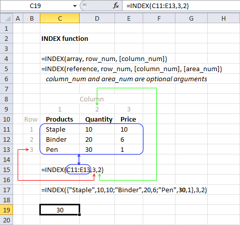
The column_num argument allows you to choose a column from which to return a value. This argument is optional, for example, if you only have values in a single column.
The cell range C11:E13 is two-dimensional meaning there are multiple rows and columns. In this example, the value in the third row and the second column is returned.
I have greyed out the row and column numbers in the image above, this makes it easier to see that value 30 is where row 3 and column 2 interesects.
The following formula contains an array of constants. It retrieves the value from the third row and second column.
{"Staple", 10, 10; "Binder", 20, 6; "Pen", 30, 1} has values separated by commas and semicolons meaning commas separate values between columns and semicolons separate values between rows.
Read more: Looking up data in a cross reference table
8. How to use the [area_num] argument
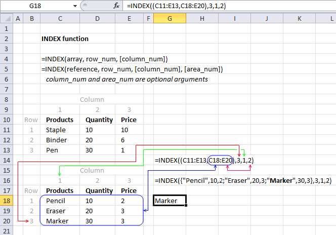
The INDEX function lets you have multiple cell references in the first argument, the area_num argument allows you to pick a cell range in the reference argument.
INDEX(reference, row_num, [column_num], [area_num])
The following formula has two references pointing to two different cell ranges.
The area_num selects from which cell reference to return a value. In this example, area_num is two therefore the second cell reference is used. The item in the third row and the first column is returned.
The INDEX function returns a #VALUE! error if you reference a cell range on another worksheet, however, there is a workaround.
9. How to return the entire row in a given cell range
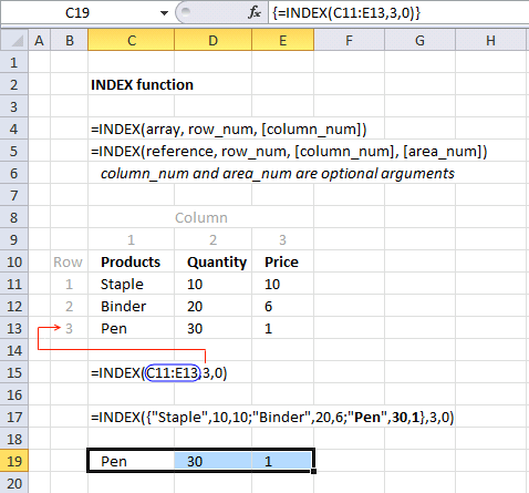
The INDEX function is also capable of returning an array from a column, row, and both columns and rows. The following formula demonstrates how to extract all values from row three:
The formula in cell C19:E19 is an array formula, here is how to enter an array formula.
- Select cell range C19:E19.
- Type =INDEX(C11:E13,3,0) in formula bar.
- Press and hold CTRL + SHIFT simultaeously.
- Press Enter.
- Release all keys.
9.1 How to return an column of values in a given cell range
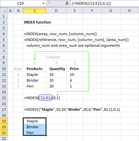
The example above demonstrates an array formula that returns all values from column 1 from cell range C11:E13.
9.2 How to return the entire specified cell range
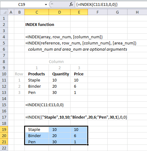
The example above returns all values from a two-dimensional cell range. The following array formula returns all values on all rows and columns from a cell range.
The zeros in both the row_num and column_num arguments allow you to get all values in the specified cell range. The example above uses C11:E13 as the array argument, all values in C11:E13 are returned.
10. How to build a dynamic cell reference
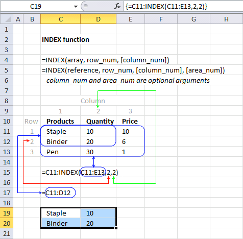
The INDEX function can also be used to create a cell reference, for example, a dynamic range created by a formula in a named range.
Array formula in cell range C19:D20:
Explaining formula
Step 1 - Calculate cell reference
INDEX(C11:E13,2,2)
returns cell reference D12.
Step 2 - Build new cell reference
The colon lets you append two single cell references creating a larger cell range reference.
C11:INDEX(C11:E13,2,2)
becomes C11:D12
and returns {"Staple",10;"Binder",20}.
Final note
There are some magic things you can do with the array argument if you use an Excel version prior to Excel 365. See this post: No more array formulas?
11. Function not working

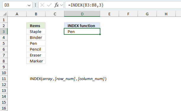
The INDEX returns a #REF! error if the row_num or col_num arguments points to a cell outside the given cell reference. Change the row_num or col_num so it points to a cell insdie the given array argument.
The example above shows the INDEX function in cell D3, it returns #REF error because the row_num points to a cell outside cell range B3:B8. Cell range B3:B8 contains six cells, the row_num argument points to cell 12.

An error is shown if the source cell contains an error value. The image above shows the INDEX function in cell D3, it retrieves the value from cell B4, however, B4 contains a #DIV/0 error. The INDEX function in cell D3 returns the same error.
Make sure your source data is free from errors.

The INDEX function returns a #VALUE! error if the number of arguments are wrong or the arguments contain text values. The image above shows the INNDEX function in cell D3 returning a #VALUE! error. The second argument row_num is a text value and not a number which is not valid.

The INDEX function returns a #VALUE! error if a reference points to a cell range located on another worksheet. The image above shows the INDEX function in cell D3, the first cell reference points to B3:B8, however, the second cell reference points to cell range B3:D5 on another worksheet. This is not allowed, a workaround is required.

The image above shows the workaround in cell D3, this formula allows you to use cell references pointing to other worksheets.
Formula in cell D3:
11.1 Explaining formula
Step 1 - Select cell reference
The CHOOSE function gets a value based on a number.
Function syntax: CHOOSE(index_num, value1, [value2], ...)
CHOOSE(2,B3:B8,OFFSET!B3:D5)
returns
OFFSET!B3:D5. This is a cell reference on a worksheet named OFFSET.
Step 2 - Get value based on selected cell reference
INDEX(CHOOSE(2,B3:B8,OFFSET!B3:D5),1,3)
becomes
INDEX(OFFSET!B3:D5,1,3)
and returns "Paper".
The INDEX function gets the value on row 1 and column 3 in cell range OFFSET!B3:D5.
12. Can you replace the VLOOKUP function with the INDEX function?

Yes, you can. The image above shows the INDEX formula in cell F3 and the VLOOKUP formula in cell F8. The INDEX formula needs the MATCH function to determine the relative position of value "Pencil" in cell range B3:B8.
The VLOOKUP finds the position automatically and the formula is somewhat smaller and easier to understand, the downside is that the VLOOKUP function performs a lookup only in the leftmost column. However, the INDEX formula can easily be customized to perform a lookup in any column you like.
Formula in cell F8:
Formula in cell F3:
This example demonstrates that the INDEX formula above replaces the VLOOKUP formula, it performs the exact same task. This lets you compare the formulas and see the differences.
13. Where do I use the INDEX - MATCH functions instead of VLOOKUP?

Use the INDEX - MATCH functions when you want to lookup a value not in the leftmost column of a cell range, the VLOOKUP function can only perform a lookup in the leftmost column of the specified cell range. The image above shows an example in cell F3.
The formula looks for number 9 in column "Qty" and finds it on row 3 in cell range C3:C8, this range is not the leftmost column in cell range B3:D8. The INDEX function retrieves the value from row 3 and column in B3:C8 which is "Pen".
Explaining formula
Step 1 - Calculate the relative position of number 9 in C3;C8
The MATCH function returns the relative position of an item in an array that matches a specified value in a specific order.
Function syntax: MATCH(lookup_value, lookup_array, [match_type])
MATCH(9,C3:C8,0)
becomes
MATCH(9,{12;8;9;10;4;11},0)
and returns 3. 9 has the relative position three in the array.
Step 2 - Get value
The INDEX function returns a value or reference from a cell range or array, you specify which value based on a row and column number.
Function syntax: INDEX(array, [row_num], [column_num])
INDEX(B3:D8,MATCH(9,C3:C8,0),1)
returns "Pen" in cell F3.
14. Excel file
Useful resources
INDEX function - Microsoft
INDEX function - ExcelJet
Index Match Formula
15. Get the latest revision
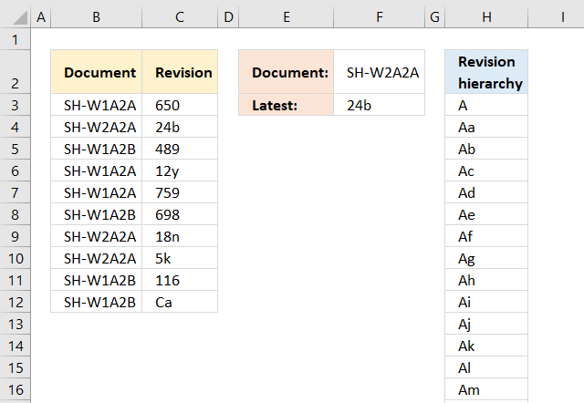
Column B contains document names, many of them are duplicates. The adjacent column C has the revision of the documents in alphanumeric format.
The array formula in cell F3 returns the latest revision based on the document name in cell F2.
The issue here is that the revisions may contain both letters and numbers and Excel can't extract the latest revision based on sorting from A to Z, that is why the revision hierarchy is in column H to guide Excel.
To enter an array formula, type the formula in a cell then press and hold CTRL + SHIFT simultaneously, now press Enter once. Release all keys.
The formula bar now shows the formula with a beginning and ending curly bracket telling you that you entered the formula successfully. Don't enter the curly brackets yourself.
Explaining array formula in cell F3
The IF function extracts revisions based on the document name in cell F2.
IF(F2=$B$3:$B$12, $C$3:$C$12, "")
becomes IF("SH-W2A2A"={"SH-W1A2A"; "SH-W2A2A"; "SH-W1A2B"; "SH-W1A2A"; "SH-W1A2A"; "SH-W1A2B"; "SH-W2A2A"; "SH-W2A2A"; "SH-W1A2B"; "SH-W1A2B"},{"650"; "24b"; "489"; "12y"; "759"; "698"; "18n"; "5k"; "116"; "Ca"},"")
and returns {"";"24b";"";"";"";"";"18n";"5k";"";""}.
The MATCH function then finds the position of each value in the array, if a value is not found the function returns an #N/A error.
MATCH(IF(F2=$B$3:$B$12, $C$3:$C$12, ""), $H$3:$H$2456,0)
becomes
MATCH({"";"24b";"";"";"";"";"18n";"5k";"";""}, $H$3:$H$2456,0)
and returns {#N/A; 1326; #N/A; #N/A; #N/A; #N/A; 1176; 822; #N/A; #N/A}
A higher number means a later revision.
The IFERROR function converts error values to blanks.
IFERROR(MATCH(IF(F2=$B$3:$B$12, $C$3:$C$12, ""), $H$3:$H$2456,0), "")
becomes
IFERROR({#N/A; 1326; #N/A; #N/A; #N/A; #N/A; 1176; 822; #N/A; #N/A}, "")
and returns {""; 1326; ""; ""; ""; ""; 1176; 822; ""; ""}.
The MAX function gets the largest number in the array, it corresponds to the latest revision.
MAX(IFERROR(MATCH(IF(F2=$B$3:$B$12, $C$3:$C$12, ""), $H$3:$H$2456, 0), ""))
becomes
MAX({""; 1326; ""; ""; ""; ""; 1176; 822; ""; ""})
and returns 1326.
The INDEX function then returns the latest revision value.
INDEX($H$3:$H$2456, MAX(IFERROR(MATCH(IF(F2=$B$3:$B$12, $C$3:$C$12, ""), $H$3:$H$2456,0), "")))
becomes
INDEX($H$3:$H$2456, 1326)
and returns 24b in cell F3.
Get Excel *.xlsx file
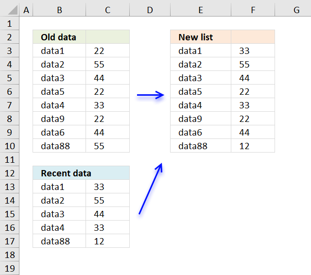
16. Create a list with most recent data available
A3 data2 B3 55
A4 data3 B4 44
A5 data5 B5 22
A6 data4 B6 33
A7 data9 B7 22
A8 data6 B8 44
A9 data88 B9 55in the second setD2 data1 E2 33
D3 data2 E3 55
D4 data3 E4 44
D5 data4 E5 33
D6 data88 E6 12the new list should change B2 from 22 to 33.
If there is no change it shows the first sets result . if there is a change it reports from the second set.
To complicate it... the first set of data is twice as long as the second one. not all data is in the second set and finally the lists are not sorted and cant be.
Formula in F3:
copied down as far as needed.
Explaining formula in cell B13
Step 1 - Count given value in cell range
The COUNTIF function counts cells based on a condition, it will return 1 if the value exists in cell range $B$13:$B$17.
COUNTIF($B$13:$B$17, E3)=0
becomes
COUNTIF({"data1";"data2";"data3";"data4";"data88"},"data1")=0
becomes
1=0 and returns FALSE.
Step 2 - Which cell range?
The IF function determines from which cell range the formula retrieves the value needed.
IF(COUNTIF($B$13:$B$17, E3)=0, INDEX($C$3:$C$10, MATCH(E3, $B$3:$B$10, 0)), INDEX($C$13:$C$17, MATCH(E3, $B$13:$B$17, 0)))
becomes
IF(FALSE, INDEX($C$3:$C$10, MATCH(E3, $B$3:$B$10, 0)), INDEX($C$13:$C$17, MATCH(E3, $B$13:$B$17, 0)))
and returns
INDEX($C$13:$C$17, MATCH(E3, $B$13:$B$17, 0))
Step 3 - Get value
The MATCH function returns the relative position of a value in a cell range or array.
INDEX($C$13:$C$17, MATCH(E3, $B$13:$B$17, 0))
becomes
INDEX($C$13:$C$17, 1)
The INDEX function returns a value based on a row number (and a column number if needed).
INDEX($C$13:$C$17, 1)
returns 33 in cell F3.
Get Excel *.xlsx file
Create-a-column-with-most-recent-data-in-excel.xlsx
'INDEX' function examples

First, let me explain the difference between unique values and unique distinct values, it is important you know the difference […]

This post explains how to lookup a value and return multiple values. No array formula required.

Array formulas allows you to do advanced calculations not possible with regular formulas.
Functions in 'Lookup and reference' category
The INDEX function function is one of 25 functions in the 'Lookup and reference' category.
Excel function categories
Excel categories
13 Responses to “How to use the INDEX function”
Leave a Reply
How to comment
How to add a formula to your comment
<code>Insert your formula here.</code>
Convert less than and larger than signs
Use html character entities instead of less than and larger than signs.
< becomes < and > becomes >
How to add VBA code to your comment
[vb 1="vbnet" language=","]
Put your VBA code here.
[/vb]
How to add a picture to your comment:
Upload picture to postimage.org or imgur
Paste image link to your comment.
[...] INDEX function returns a value of the cell at the intersection of a particular row and column, in a given range. [...]
[...] INDEX(array,row_num,[column_num]) Returns a value or reference of the cell at the intersection of a particular row and column, in a given range [...]
[...] INDEX(array,row_num,[column_num]) Returns a value or reference of the cell at the intersection of a particular row and column, in a given range [...]
[…] INDEX(array,row_num,[column_num]) Returns a value or reference of the cell at the intersection of a particular row and column, in a given range […]
[…] INDEX(array,row_num,[column_num]) Returns a value or reference of the cell at the intersection of a particular row and column, in a given range […]
[…] INDEX(array,row_num,[column_num]) Returns a value or reference of the cell at the intersection of a particular row and column, in a given range […]
Hi there
I have a list of serial numbers in column A. I need to bath them in batches of 20 and hence custom naming the batches with the number increment increasing.
Eg Column A Column B
987654 vodacom_03022015_75062
987655 vodacom_03022015_75062
so column A 2o rows will have same batch name and number
next 20 will increase number in column b by 1...
PLEase help
If you wish for to get a good deal from this post
then you have to apply these strategies to
your won website.
SIR MY NAME IS JAGBIR SINGH.
I AM JUST CONFUSE FOR TAKING INDEX FORMULA INSTEAD OF V LOOKUP
BY VLOOKUP WE CAN TAKE DATA OF ANOTHER SHEET INTO ONE SHEET.
BUT BY INDEX FORMULA I AM UNABLE TO DO THAT.
PLEASE SUGGEST ME HOW ITS WORK FOR TWO SHEET.
JAGBIR SINGH,
This formula returns a value from sheet2:
INDEX(Sheet2!$A$2:$A$10, MATCH($A$2,Sheet2!$B$2:$B$10,0))
hi sir i have confusion on some matter to sortin data from list of given names
hello sir,
i have a column with various data and i want to show it in 1 cell.
https://gyazo.com/a1b23e2530007a4e9d25ea4b711d8bbb
can you help me how to do it
thanks
In Example 4 - Area_num argument, the first range (C11:E13) does not do any thing, why we need it there?
=INDEX(C18:E20,3,1) does the same and simple.
So, what's the purpose of =INDEX((C11:E13,C18:E20),3,1,2)?
Thank you!