How to use the IF function
What is the IF function?
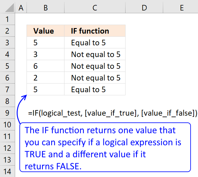
The IF function returns one value if the logical test is TRUE and another value if the logical test is FALSE.
Table of Contents
- Syntax
- Example
- What is a logical expression?
- What logical operators can you use in the logical expression?
- Use an Excel function to perform a logical test
- Cell is blank
- Cell is not blank
- Cell contains an error
- Cell is a text value
- Cell is a number
- False do nothing
- Greater than
- Smaller than
- Equals
- Equals multiple values
- Not equal
- Begins with
- Ends with
- Contains
- Contains any text
- Exact match case sensitive
- AND OR
- Between two sheets
- Copy cell value
- Add value
- Keep value
- Keep blank
- Based on cell color
- How to work with multiple values
- Between two numbers
- Get Excel *.xlsx file
- How to use nested functions
- OR function
- Check if there is at least one number above a given value
- How to check if there is a blank value in a cell range
- Function not working
- Get Excel file
1. Syntax
IF(logical_test, [value_if_true], [value_if_false])
| logical_test | Required. The logical expression determines what value the IF function returns. Excel evaluates all numerical values positive or negative to TRUE except 0 (zero) that equals FALSE. |
| [value_if_true] | Optional. The value the IF function returns if the logical expression evaluates to TRUE. If omitted 0 (zero) is returned. |
| [value_if_false] | Optional. The value the IF function returns if the logical expression evaluates to FALSE. If omitted 0 (zero) is returned. |
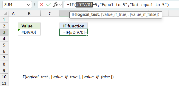
3. Example

This formula is using the IF function, which allows you to make a logical comparison between a value and and a given condition, and return one value for a TRUE result and another for a FALSE result.
The syntax of the IF function is:
=IF(logical_test, value_if_true, value_if_false)
The logical_test argument is the condition that we want to evaluate. The value_if_true argument is the value that we want to return if the logical_test is TRUE. The value_if_false argument is the value that you want to return if the logical_test is FALSE.
In this formula, the logical_test is B3=5, which means we are checking if the value in cell B3 is equal to 5. The value_if_true is "Equal to 5", which means we want to display the text "Equal to 5" if B3=5. The value_if_false is "Not equal to 5", which means we want to display the text "Not equal to 5" if B3 is not equal to 5.
So, the formula will return "Equal to 5" if B3=5, and "Not equal to 5" otherwise.

Formula in cell C3:
For example, if B3 contains 5, the formula will return "Equal to 5". If B3 contains 4, the formula will return "Not equal to 5".
Text values like "Equal to 5" and "Not equal to 5" must be enclosed in double quotes ("") in the IF function. However, numeric values like 5 do not need quotes.
4. What is a logical expression?
The logical_test argument in the IF function determines the outcome meaning if the second argument [value_if_true] or third argument [value_if_false] will be returned or calculated.
Logical operators are often used in the logical_test argument, they return TRUE or FALSE:
< less than sign
> greater than sign
= equal sign
<> not equal to
<= less than or equal to
>= greater than or equal to
Functions that return a number also work a logical_test, here are a few examples:
COUNT function
SUM function
COUNTIF function
Functions that return TRUE or FALSE are also valid logical expressions:
ISERROR function
ISNUMBER function
ISODD function
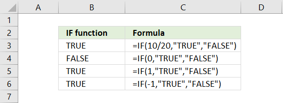
Boolean value TRUE or FALSE are valid outcomes, however, their numerical equivalents are also valid. For example, 0 (zero) is evaluated as FALSE and all other numerical values, even negative values, are evaluated as TRUE.
4.1 Can a decimal number be used as a logical expression?
Formula in cell B3:
The logical_test argument in the formula above is 10/20 which equals 0.5. 0.5 is not equal to 0 (zero) so the formula returns TRUE in cell B3.
4.2 Is 0 (zero) equivalent to boolean value FALSE in a logical expression?
Formula in cell B4:
The logical_test argument in cell B4 above is 0 (zero). 0 (zero) equals 0 (zero) so the formula returns FALSE in cell B3.
4.3 Is 1 equivalent to boolean value TRUE in a logical expression?
Formula in cell B5:
The logical_test argument in the formula above is 1. 1 is not equal to 0 (zero) so the formula returns TRUE in cell B3.
4.4 Is -1 (negative number) equivalent to boolean value TRUE in a logical expression?
Formula in cell B6:
The logical_test argument in cell B6 above is -1. -1 is not equal to 0 (zero) and the formula returns TRUE in cell B3.
4.5 What happens if a text string is used in the logical expression?
The formula above returns #VALUE! error which means that text strings are not allowed as a logical test, however a logical expression using text strings are fine, see example below.
This formula will return TRUE because "A" is equal to "A".
5. What logical operators can you use in the logical expression?
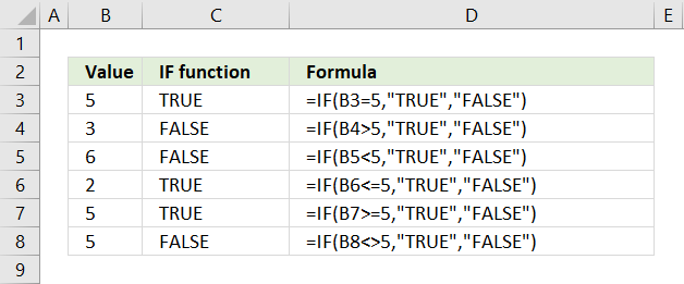
The logical_test argument allows you to use comparison operators, these characters let you to do more advanced comparisons than the equal sign.
- = (equal sign)
- < less than
- > greater than
- <= less than or equal to
- >= greater than or equal to
- <> not equal
Formula in cell C3:
This formula compares the value in cell B3 with number 5, if equal TRUE is returned. Note that this formula is only for demonstration purposes, you can use this formula in cell C3 to get the same result =B3=5.
If you change the value in cell B3 the formula in cell C3 instantly recalculates and returns TRUE or FALSE based on the outcome of the logical_test.
Formula in cell C4:
The formula in cell C4 checks if the value in cell B4 is larger than 5, cell B4 contains 3 and 3 is not larger than 5 so the formula returns FALSE.
Formula in cell C5:
This formula evaluates if the value in cell B5 is smaller than 5, the image above shows that cell B5 contains number 6. 6 is not smaller than 5 and the formula returns FALSE.
Formula in cell C6:
The formula in cell C6 evaluates if the value in cell B6 is smaller than or equal to 5. Cell B6 contains 2, see image above, and 2 is smaller than or equal to 5. The formula returns TRUE in cell C6.
Formula in cell C7:
This formula checks if value in cell B7 is larger than or equal to 5, cell B7 contains 5 and 5 is equal to 5. The formula returns TRUE in cell C7.
Formula in cell C8:
The formula in cell C8 assesses if value in cell B8 is not equal to 5, cell B8 contains 5. 5 is equal to 5 and the formula returns FALSE in cell C8.
6. Use an Excel function to perform a logical test
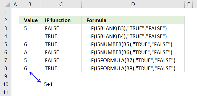
You are not limited to comparison operators when dealing with the logical_test argument, any function that returns TRUE or FALSE can be used.
The picture above shows a formula in cell C3 that evaluates if cell B3 is blank. It is not blank so it returns FALSE.
Cell B4 is blank and the IF function returns TRUE in cell C4.
The following formula uses the ISNUMBER function to identify the value in cell B5.
The formula in cell C5 returns TRUE because the value in cell B5 is 6 and that is a number.
Cell C7 and C8 contain formulas that test if B7 and B8 contain a formula. Formula in cell C8 returns TRUE, cell B8 contains this formula =5+1.
Check out the functions in the Information category, many of them return TRUE or FALSE.
7. How to check if a cell is blank?

The image above demonstrates the IF function in cell C3. It checks if the adjacent cell on the same row in column B is blank. If not blank the value itself is returned.
Formula in cell C3:
Cell reference B3 is a relative cell reference meaning it changes accordingly when you copy cell C3 and paste it to cells below.
Explaining formula in cell C3
Step 1 - Logical expression
The logical expression contains the equal sign. It checks if one value is equal to another value and returns boolean values TRUE or FALSE.
"" is the same as nothing or an empty cell.
B3=""
becomes
5=""
and returns FALSE. 5 is not equal to nothing.
Step 2 - Evaluate IF function
The second argument in the IF function is returned if the logical expression returns TRUE and the third is returned if FALSE.
IF(logical_test, [value_if_true], [value_if_false])
IF(B3="","Blank",B3)
becomes
IF(FALSE,"Blank",B3)
becomes
IF(FALSE,"Blank",5)
and returns 5 or the value itself in cell B3.
8. How to check if a cell is not blank?
The image above demonstrates the IF function in cell C3. It checks if the adjacent cell on the same row in column B is not blank. If not blank the value itself is returned.
Formula in cell C3:
Cell reference B3 is a relative cell reference meaning it changes accordingly when you copy cell C3 and paste it to cells below.
Explaining formula in cell C3
Step 1 - Logical expression
The logical expression contains two logical operaters, the first one is smaller than and the seconmd is larger than. When you combine these you get not equal to.
"" is the same as nothing or an empty cell.
B3<>""
becomes
5<>""
and returns TRUE. 5 is not equal to nothing.
Step 2 - Evaluate IF function
The second argument in the IF function is returned if the logical expression returns TRUE and the third is returned if FALSE.
IF(logical_test, [value_if_true], [value_if_false])
IF(B3<>"",B3,"Blank")
becomes
IF(TRUE,B3,"Blank")
becomes
IF(TRUE,5,"Blank")
and returns 5 or the value itself in cell B3.
9. How to check if a cell contains an error?

The image above demonstrates an IF function in cell C3. It checks if the adjacent cell on the same row in column B contains an error value. The formula returns "Error" if true and the value itself if false.
Formula in cell C3:
Cell reference B3 is a relative cell reference meaning it changes accordingly when you copy cell C3 and pastes it to cells below.
Explaining formula in cell C3
Step 1 - Logical expression
The ISERROR function returns TRUE if the cell contains an error and FALSE if not.
ISERROR(B3)
becomes
ISERROR(5)
and returns FALSE.
Step 2 - Evaluate IF function
The second argument in the IF function is returned if the logical expression returns TRUE and the third is returned if FALSE.
IF(logical_test, [value_if_true], [value_if_false])
IF(ISERROR(B3), "Error", B3)
becomes
IF(FALSE, "Error", B3)
becomes
IF(FALSE, "Error", 5)
and returns 5.
10. How to check if a cell is a text value?

The image above shows an IF function in cell C3 that checks if the adjacent cell on the same row in column B is a text value. The formula returns "Text" if true and "Not text" if false.
Formula in cell C3:
Cell reference B3 is a relative cell reference meaning it changes accordingly when you copy cell C3 and pastes it to cells below.
Explaining formula in cell C3
Step 1 - Logical expression
ISTEXT(B3)
becomes
ISTEXT(5)
and returns boolean FALSE.
Step 2 - Evaluate IF function
The ISTEXT function returns True if the argument is text and False if not.
IF(ISTEXT(B3), "Text", "Not text")
becomes
IF(False, "Text", "Not text")
and returns "Not text" in cell C3.
11. How to check if a cell is a number?

The image above shows an IF function in cell C3 that checks if the adjacent cell on the same row in column B is a text value. The formula returns "Text" if true and "Not text" if false.
Formula in cell C3:
Cell reference B3 is a relative cell reference meaning it changes accordingly when you copy cell C3 and pastes it to cells below.
Explaining formula in cell C3
Step 1 - Logical expression
The ISNUMBER function returns TRUE if the argument is a number and FALSE if not.
ISNUMBER(B3)
becomes
ISNUMBER(5)
and returns boolean TRUE.
Step 2 - Evaluate IF function
IF(ISTEXT(B3), "Text", "Not text")
becomes
IF(False, "Text", "Not text")
and returns "Not text" in cell C3.
12. False do nothing

The formula in cell C3 checks if the value in cell B3 is equal to 5, if so add 5 to the number in cell B3. If cell B3 is not equal to 5 do nothing.
Formula in cell C3:
Cell reference B3 is a relative cell reference meaning it changes accordingly when you copy cell C3 and pastes it to cells below.
Explaining formula in cell C3
Step 1 - Logical expression
The equal sign lets you compare two or more values, the expression returns TRUE or FALSE.
B3=5
becomes
5=5
and returns TRUE.
Step 2 - Evaluate IF function
The second argument is returned if the logical expression returns TRUE and the third argument is returned if FALSE. The third argument is "" which is nothing. The cell is empty. The IF function returns 0 (zero) if you leave the third argument empty.
IF(B3=5,B3+5,"")
becomes
IF(TRUE,B3+5,"")
becomes
IF(TRUE,5+5,"")
and returns 10 in cell C3.
13. Greater than

The formula in cell C3 checks if the value in cell B3 is larger than cell C7, if so return the number in cell B3. If cell B3 is not larger than cell C7 then do nothing.
Formula in cell C3:
Cell reference B3 is a relative cell reference meaning it changes accordingly when you copy cell C3 and pastes it to cells below.
Explaining formula in cell C3
Step 1 - Logical expression
The larger than character lets you check if cell B3 is larger than cell C7, it returns TRUE if so. FALSE if not.
B3>$C$7
becomes
5>5
and returns FALSE.
Step 2 - Evaluate IF function
IF(B3>$C$7, B3, "")
becomes
IF(FALSE, B3, "")
becomes
IF(FALSE, 5, "")
and returns "" (nothing).
14. Smaller than

The formula in cell C3 checks if the value in cell B3 is smaller than cell C7, if so return the number in cell B3. If cell B3 is not smaller than cell C7 then do nothing.
Formula in cell C3:
Cell reference B3 is a relative cell reference meaning it changes accordingly when you copy cell C3 and pastes it to cells below.
Explaining formula in cell C3
Step 1 - Logical expression
The smaller than character lets you check if cell B3 is smaller than cell C7, it returns TRUE if so. FALSE if not.
B3<$C$7
becomes
5<5
and returns FALSE.
Step 2 - Evaluate IF function
IF(B3<$C$7, B3, "")
becomes
IF(FALSE, B3, "")
becomes
IF(FALSE, 5, "")
and returns "" (nothing).
15. Equals

The formula in cell C3 checks if the value in cell B3 is equal to value in cell C7, if so return "Yes". If cell B3 is not equal to cell C7 then return "No".
Formula in cell C3:
Cell reference B3 is a relative cell reference meaning it changes accordingly when you copy cell C3 and pastes it to cells below.
Explaining formula in cell C3
Step 1 - Logical expression
The equal character lets you check if cell B3 is equal to the value in cell C7, it returns TRUE if so. FALSE if not.
B3=$C$7
becomes
5=4
and returns FALSE.
Step 2 - Evaluate IF function
IF(B3=$C$7, "Yes", "No")
becomes
IF(FALSE, "Yes", "No")
becomes
IF(FALSE, "Yes", "No")
and returns "No".
16. Cell equals any of multiple values (OR logic)

The formula in cell C3 checks if the value in cell B3 is equal to any of the values in cell range C9:C11. If one value is equal then the formula returns "Yes" if not "No".
Formula in cell C3:
Cell reference B3 is a relative cell reference meaning it changes accordingly when you copy cell C3 and pastes it to cells below.
Explaining formula in cell C3
Step 1 - Logical expression
You can use logical operators to compare one value to multiple values, the result is an array with multiple boolean values TRUE or FALSE.
B3=$C$7:$C$11
becomes
"A"={"D";"C";"F"}
and returns
{FALSE; FALSE; FALSE}. "A" is not equal to "D", "C" or "F".
Step 2 - Evaluate OR function
The OR function returns TRUE if at least one boolean value in the array is TRUE. The OR function returns FALSE if all values in the array are FALSE.
OR(B3=$C$7:$C$11)
becomes
OR({FALSE; FALSE; FALSE})
and returns FALSE.
Step 3 - Evaluate IF function
IF(OR(B3=$C$7:$C$11), "Yes", "No")
becomes
IF(FALSE, "Yes", "No")
and returns "No".
Recommended links: If cell equals value from list | If cell contains text from list | IF with OR function | If cell contains text
17. Not equal

The formula in cell C3 checks if the value in cell B3 is not equal to the value in cell C7, if so return "Yes". If cell B3 is not equal to cell C7 then return "No".
Formula in cell C3:
Cell reference B3 is a relative cell reference meaning it changes accordingly when you copy cell C3 and pastes it to cells below.
Explaining formula in cell C3
Step 1 - Logical expression
The less and greater than characters combined lets you check if cell B3 is not equal to the value in cell C7, it returns TRUE if so. FALSE if not.
B3<>$C$7
becomes
5<>4
and returns FALSE.
Step 2 - Evaluate IF function
IF(B3<>$C$7, "Yes", "No")
becomes
IF(TRUE, "Yes", "No")
and returns "Yes".
18. Begins with

The formula in cell C3 checks if the value in cell B3 begins with the value in cell C7, if so return "Yes". If cell B3 does not end with value in cell C7 then return "No".
Note that the equal sign is not evaluating text strings with regard to upper and lower letters, in other words, the equal sign is not case sensitive.
Formula in cell C3:
Cell reference B3 is a relative cell reference meaning it changes accordingly when you copy cell C3 and pastes it to cells below.
Explaining formula in cell C3
Step 1 - Count characters
The LEN function counts the number of characters in a string.
LEN($C$7)
becomes
LEN("Gr")
and returns 2.
Step 2 - Return k-th characters from left
The LEFT function returns a given number of characters from left.
LEFT(B3, LEN($C$7))
becomes
LEFT("Red", 2)
and returns "Re".
Step 3 - Logical test
LEFT(B3, LEN($C$7))=$C$7
becomes
"Re"="Gr"
and returns FALSE.
Step 4 - Evaluate IF function
IF(LEFT(B3, LEN($C$7))=$C$7, "Yes", "No")
becomes
IF(FALSE, "Yes", "No")
and returns "No" in cell C3.
19. Ends with

The formula in cell C3 checks if the value in cell B3 ends with the value in cell C7, if so return "Yes". If cell B3 does not end with value in cell C7 then return "No".
Formula in cell C3:
Cell reference B3 is a relative cell reference meaning it changes accordingly when you copy cell C3 and pastes it to cells below.
Explaining formula in cell C3
Step 1 - Count characters
The LEN function counts the number of characters in a string.
LEN($C$7)
becomes
LEN("ue")
and returns 2.
Step 2 - Return k-th characters from left
The RIGHT function returns a given number of characters from the right.
RIGHT(B3, LEN($C$7))
becomes
RIGHT("Red", 2)
and returns "ed".
Step 3 - Logical test
RIGHT(B3, LEN($C$7))=$C$7
becomes
"ed"="ue"
and returns FALSE.
Step 4 - Evaluate IF function
IF(RIGHT(B3, LEN($C$7))=$C$7, "Yes", "No")
becomes
IF(FALSE, "Yes", "No")
and returns "No" in cell C3.
20. Cell contains a given string

The formula in cell C3 checks if the value in cell B3 contains the string in cell C7, if so return "Yes". If cell B3 does not contain the string in cell C7 then return "No".
Formula in cell C3:
Cell reference B3 is a relative cell reference meaning it changes accordingly when you copy cell C3 and pastes it to cells below.
Explaining formula in cell C3
Step 1 - Check if value contains string
The COUNTIF function allows you to count cells matching a specific value, however, it also allows you to count cells containing a specific string.
You need to append the asterisk character before and after the string.
COUNTIF(B3, "*"&$C$7&"*")
becomes
COUNTIF("Red", "*r*")
and returns 1. This means that the string is found in cell B3. 1 is equal to TRUE and 0 (zero) is equal to FALSE.
Step 2 - Evaluate IF function
IF(COUNTIF(B3, "*"&$C$7&"*"), "Yes", "No")
becomes
IF(1, "Yes", "No")
and returns "Yes" in cell C3.
21. Contains any text

The formula in cell C3 checks if the value in cell B3 is a number by multiplying with 1, if so return "Yes". If cell B3 does not contain the string in cell C7 then return "No".
Formula in cell C3:
Cell reference B3 is a relative cell reference meaning it changes accordingly when you copy cell C3 and pastes it to cells below.
Explaining formula in cell C3
Step 1 - Check if value contains a text string
We get an error if we try to multiply a text string with a number, we can use that technique to identify numerical values.
B3*1
becomes
23145256*1
and returns 23145256.
Step 2 - Check error
The ISERROR function returns TRUE if argument is an error value and FALSE if not.
ISERROR(B3*1)
becomes
ISERROR(23145256)
and returns FALSE.
Step 3 - Evaluate IF function
IF(ISERROR(B3*1),"Contains text", "No text")
becomes
IF(FALSE,"Contains text", "No text")
and returns "No text".
22. Exact match case sensitive

The formula in cell C3 checks if the value in cell B3 is equal to the value in cell C11, upper and lower case letters are also evaluated. If a case sensitive match is found then return "Yes" otherwise return "No".
Formula in cell C3:
Cell reference B3 is a relative cell reference meaning it changes accordingly when you copy cell C3 and pastes it to cells below.
Explaining formula in cell C3
Step 1 - Check if value equals text string
The EXACT function checks if two values are precisely the same, it returns TRUE or FALSE. The EXACT function also considers upper case and lower case letters when evaluating arguments.
EXACT(B3,$C$11)
becomes
EXACT("France","FrancE")
and returns FALSE.
Step 2 - Evaluate IF function
IF(EXACT(B3,$C$11), "Yes", "No")
becomes
IF(FALSE, "Yes", "No")
and returns "No" in cell C3.
23. AND logic

The image above shows a formula in cell D3 that checks if the value in cell B3 is equal to the value in cell C11 and C3 is equal to C12. Both conditions must be met to return "Yes" otherwise return "No".
Formula in cell D3:
Cell reference B3 and C3 are relative cell references meaning they change accordingly when you copy cell D3 and pastes it to cells below.
Explaining formula in cell C3
Step 1 - Evaluate first logical expression
B3=$C$11
becomes
"Blue"="Green"
and returns FALSE.
Step 2 - Evaluate second logical expression
C3=$C$12
becomes
5=8
and returns FALSE.
Step 3 - Evaluate AND function
The AND function returns TRUE if all arguments return TRUE.
AND(B3=$C$11,C3=$C$12)
becomes
AND(FALSE, FALSE)
and returns FALSE.
Step 4 - Evaluate IF function
IF(AND(B3=$C$11,C3=$C$12),"Yes","No")
becomes
IF(FALSE,"Yes","No")
and returns "No" in cell D3.
24. Between two worksheets?

The image above shows a formula in cell C3 that checks if the value in cell B3 is equal to the value in cell B3 in worksheet 'AND logic'. Note that single quotation marks are used if the worksheet name contains a space character.
Formula in cell D3:
Cell reference B3 is a relative cell references meaning it changes accordingly when you copy cell C3 and pastes it to cells below.
Explaining formula in cell C3
Step 1 - Evaluate logical expression
'AND logic'!B3 is a cell reference pointing to cell B3 in worksheet 'AND logic'.
B3='AND logic'!B3
becomes
"Blue"="Blue"
and returns TRUE.
Step 2 - Evaluate IF function
IF(B3='AND logic'!B3, "Yes", "No")
becomes
IF(TRUE, "Yes", "No")
and returns "Yes" in cell D3.
25. Copy cell value?

The image above shows a formula in cell D3 that copies cell B3 if cell C3 is equal to "Yes". Nothing is returned if not equal to "Yes".
Formula in cell D3:
Cell reference B3 and C3 are relative cell references meaning they change accordingly when you copy cell D3 and pastes it to cells below.
Explaining formula in cell C3
Step 1 - Evaluate logical expression
C3="Yes"
becomes
"Yes"="Yes"
and returns TRUE.
Step 2 - Evaluate IF function
IF(C3="Yes",B3,"")
becomes
IF(TRUE, "A", "")
and returns "A" in cell D3.
26. Add value

The image above shows a formula in cell C3 that adds the value in cell C7 to cell B3 if cell B3 is equal to 5. Nothing "" is returned if not equal to 5.
Formula in cell D3:
Cell reference B3 is a relative cell references meaning it changes accordingly when you copy cell C3 and pastes it to cells below.
Explaining formula in cell C3
Step 1 - Evaluate logical expression
B3=5
becomes
4=5
and returns FALSE.
Step 2 - Evaluate IF function
IF(B3=5,B3+$C$7,"")
becomes
IF(FALSE,B3+$C$7,"")
becomes
IF(FALSE,4+5,"")
becomes
IF(FALSE,9,"")
and returns "" (nothing).
Check out the running total here: How to create a running total (SUM function)?
27. Keep value

The image above shows a formula in cell C3 that keeps the value in cell B3 if the value is equal to a condition.
Formula in cell D3:
Cell reference B3 is a relative cell references meaning it changes accordingly when you copy cell C3 and pastes it to cells below.
Explaining formula in cell C3
Step 1 - Evaluate logical expression
B3=5
becomes
4=5
and returns FALSE.
Step 2 - Evaluate IF function
IF(B3=5,B3,"")
becomes
IF(FALSE,4,"")
and returns "" (nothing) in cell C3.
28. Keep blank

The image above shows a formula in cell C3 that keeps the blank, if no blank the value in cell C7 is added to the value in column B.
Formula in cell D3:
Cell reference B3 is a relative cell references meaning it changes accordingly when you copy cell C3 and pastes it to cells below.
Explaining formula in cell C3
Step 1 - Evaluate logical expression
B3=""
becomes
4=""
and returns FALSE.
Step 2 - Evaluate IF function
IF(B3="","", B3+$C$7)
becomes
IF(FALSE,"", 4+5)
becomes
IF(FALSE,9,"")
and returns 9 in cell C3.
29. Based on cell color

The image above shows a formula in cell C3 that checks the cell background color and if color is equal to yellow add value in cell C7 to cell B3 and return the sum to cell C3..
You must first create a named range in order to use the GET.CELL function. Here is how:
- Go to tab "Formulas" on the ribbon.
- Press with left mouse button on "Name Manager" button.
- A dialog box appears. Press with left mouse button on "New..." button.

- Another dialog box appears.

- Enter a name, I chose Color.
- Type the following formula in "Refers to:"
=GET.CELL(63,INDIRECT("rc",FALSE))
- Press with left mouse button on the OK button.
- Press with left mouse button on the "Close" button.
Now back to the worksheet, formula in cell C3:
Cell reference B3 is a relative cell references meaning it changes accordingly when you copy cell C3 and pastes it to cells below.
Note, the GET.CELL function has some serious flaws:
- Obsolete and unsupported.
- Microsoft may remove the GET.CELL function whenever they feel like it.
- It does not update when a cell background-color is changed, you need to press F9 to recalculate the formulas.
- It does not support all the millions of colors available in Excel, only around 60 colors.
I recommend that you use Conditional Formatting to color cells based on a condition and use the same condition in the IF function.
Here is an example: How to sum by color?
Explaining formula in cell C3
Step 1 - Identify cell background-color
Color=6
becomes
6=6
and returns TRUE. A yellow background-color returns 6.
Step 2 - Evaluate IF function
IF(Color=6,B3+$C$7,B3)
becomes
IF(TRUE, 4+5,4)
and returns 9. 4+5 = 9.
30. How to work with multiple values

The image above demonstrates a formula in cell F5 that uses the specified value in cell F3 to filter values from column C based on column B.
If the year in column B matches the value in cell F3 the corresponding value on the same row is used. The formula is actually performing this calculation to all values in cell range B3:B10.
Array formula in cell F5:
This is an array formula, to enter an array formula press and hold CTRL + SHIFT simultaneously after you have entered the formula in a cell. Press Enter once and then release all keys.
The formula changes and now has curly brackets surrounding the formula, like this: {=MEDIAN(IF(B3:B10=F3,C3:C10,""))}
Do not enter these characters yourself, they appear automatically. Note that Office 365 subscribers do not need to enter this as an array formula, simply enter it as a regular formula. This is a new feature in Excel called Dynamic arrays.
Explaining formula in cell F5
Step 1 - Logical expression
B3:B10=F3
becomes
{2012; 2011; 2012; 2012; 2011; 2012; 2012; 2011}=2012
and returns
{TRUE; FALSE; TRUE; TRUE; FALSE; TRUE; TRUE; FALSE}
Step 2 - Evaluate IF function
The IF function compares all values in cell range B3:B10 to the value in cell F3 and returns the corresponding value from cell range C3:C10 if they match. Nothing "" is returned if they don't match.
IF(B3:B10=F3,C3:C10,"")
becomes
IF({TRUE; FALSE; TRUE; TRUE; FALSE; TRUE; TRUE; FALSE}, C3:C10, "")
becomes
IF({TRUE; FALSE; TRUE; TRUE; FALSE; TRUE; TRUE; FALSE}, {3; 76; 56; 51; 12; 6; 13; 36}, "")
and returns {3; ""; 56; 51; ""; 6; 13; ""}.
Step 3 - MEDIAN function
The MEDIAN function returns the middle value from the array.
MEDIAN(IF(B3:B10=F3,C3:C10,""))
becomes
MEDIAN({3; ""; 56; 51; ""; 6; 13; ""})
and returns 13 in cell F5.
31. Between two numbers

The image above shows a formula in cell D3 that checks if number in cell B3 is between two numbers specified in cell C8 and C9. If not in range then return nothing "".
Formula in cell D3:
Cell reference B3 is a relative cell references meaning it changes accordingly when you copy cell C3 and pastes it to cells below.
Explaining formula in cell C3
Step 1 - Evaluate first logical expression
B3>=$C$8
becomes
4>=5
and returns FALSE.
Step 2 - Evaluate second logical expression
B3<=$C$9
becomes
4<=6
and returns TRUE.
Step 3 - Multiply logical expressions (AND logic)
The parentheses are needed to control the order of operation. We need to compare values first before multiplying boolean values.
(B3>=$C$8)*(B3<=$C$9)
becomes
FALSE*TRUE
and returns 0 (zero) which is equivalent to FALSE.
Step 4 - Evaluate IF function
IF((B3>=$C$8)*(B3<=$C$9), C3, "")
becomes
IF(0, C3, "")
and returns "" (nothing) in cell D3.
32. Based on date

The image above shows a formula in cell D3 that checks if the date in cell B3 is equal to the date in cell C8, if so return the number in cell C3.. If not then return nothing "".
Formula in cell D3:
Cell reference B3 is a relative cell references meaning it changes accordingly when you copy cell C3 and pastes it to cells below.
Note, keep in mind that dates in Excel are actually numbers formatted as dates. This makes it possible to add or subtract days, months, years, hours, and seconds to a date.
For example, number 1 is 1/1/1900 and 1/1/2000 is 36526. You can see that this is correct, type 1 in a cell. Select the cell, press CTRL + 1 to format the cell. Press with left mouse button on Date and then press OK button.

Explaining formula in cell D3
Step 1 - Compare dates
B3=$C$8
becomes
44872=44874
and returns FALSE.
Step 2 - Evaluate IF function
IF(B3=$C$8,C3,"")
becomes
IF(FALSE,44872,"")
and returns "" (nothing) in cell D3.
Useful resources
IF function - Microsoft
Using IF with AND, OR and NOT functions
IF function – nested formulas and avoiding pitfalls
33. How to use nested functions
Nested IF statements in a formula are multiple combined IF functions so more conditions and outcomes become possible. They all are more or less complicated to read and thankfully there are better alternatives.
You are allowed to use up to 254 nested IF statements but before you do that make sure you read this article, I promise you it will save you a lot of time.
Table of Contents
- How to simplify nested IF functions based on a single numerical range
- How to simplify nested IF statements based on multiple numerical ranges
- How to simplify nested IF functions based on conditions
- How to simplify nested IF functions based on date ranges
- Get Excel file
This section will provide step-by-step tutorials for your specific scenario. If you can't find what you are looking for here please comment and I will add the missing part.
33.1. How to simplify nested functions based on a numerical range

You don't need to use multiple IF statements if you want to check if a cell value is in a given numerical range, it is enough to simply use two logical expressions in the first argument.
Nested IF function formula in cell C3:
The formula above demonstrates a nested IF function. The following formula simplifies the formula above, it returns TRUE if the value in cell B3 is equal to or greater than 0 and is equal to or smaller than 10.
Formula in cell C7:
Each logical expression is encapsulated with parentheses, this makes sure that the comparisons are made before multiplying the expressions. In other words, the parentheses determine the order of calculation.
The asterisk between the logical expressions means that both logical expressions must return TRUE for the logical test argument to return TRUE.
33.1.1 Explaining formula in cell C7
The formula in cell C7 is easier to understand and troubleshoot than the formula in cell C7.
Step 1 - First logical expression
The larger than character and equal sign are logical operators, they let you compare values and returns boolean values True or False.
B3>=0
becomes
5>=0
and returns boolean value True.
Step 2 - Second logical expression
B3<=10
becomes
5<=10
and returns boolean value True.
Step 3 - Multiply logical expressions - AND logic
We must check that both conditions are met and to do that we use the asterisk to multiply the expressions.
Use parentheses to control the order of calculations, we need to compare values before we multiply.
(B3>=0)*(B3<=10)
becomes
True * True
and returns 1. 1 is the numerical equivalent to True and False is 0 (zero).
AND logic returns True only if both conditions are met.
TRUE * TRUE = TRUE (1)
TRUE * FALSE= FALSE(0)
FALSE* TRUE = FALSE(0)
FALSE* FALSE= FALSE(0)
Step 4 - Evaluate IF function
The IF function returns one value if the logical test evaluates to TRUE and another value if the logical test returns FALSE.
IF(logical_test, [value_if_true], [value_if_false])
IF((B3>=0)*(B3<=10), TRUE, FALSE)
becomes
IF(1, TRUE, FALSE)
and returns TRUE.
33.2. How to simplify nested IF statements based on numerical ranges

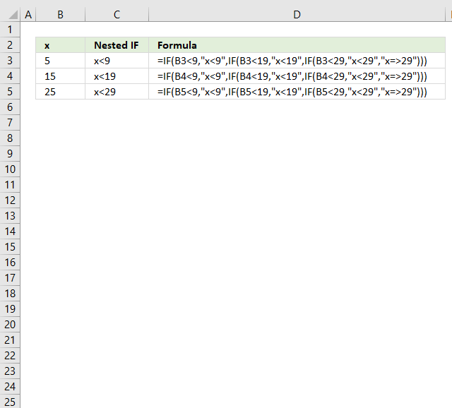
The picture above shows you nested IF statements that allow you to return different outcomes depending on the value in column B.
Nested If functions formula in cell C3:
A value equal to or greater than 0 and smaller than 10 is in "Group 1".
A value equal to or greater than 10 and smaller than 20 returns "Group 2".
A value equal to or greater than 20 and smaller than 30 returns "Group 3".
The simplified formula in cell C11:
This formula is considerably smaller and doesn't grow bigger if you need more criteria.
33.2.1 Explaining formula in cell C11
Step 1 - Build the table

The table above defines the numerical ranges and what value to return. Note, that there are no gaps between the ranges.
Step 2 - VLOOKUP function
The VLOOKUP function lets you search the leftmost column for a value and return another value on the same row in a column you specify.
VLOOKUP(lookup_value, table_array, col_index_num, [range_lookup])
lookup_value - A value.
table_array - The range you want to use, remember that the VLOOKUP function always looks in the leftmost column in your specified range.
col_index_num - The column number which contains the return value.
[range_lookup] - True or False. True - approximate match, the leftmost column must be in ascending order. False - Exact match.
Step 3 - Populate arguments
VLOOKUP(lookup_value, table_array, col_index_num, [range_lookup])
lookup_value - B11
table_array - $E$11:$F$14
col_index_num - 2
[range_lookup] - True.
VLOOKUP(lookup_value, table_array, col_index_num, [range_lookup])
becomes
VLOOKUP(B11, $E$11:$F$14, 2, TRUE)
Step 4 - Evaluate VLOOKUP function
VLOOKUP(B11, $E$11:$F$14, 2, TRUE)
becomes
VLOOKUP(5, {0, "Group 1"; 10, "Group 2"; 20, "Group 3"; 30, 0}, 2, TRUE)
and returns "Group 1" in cell C11.
The last argument TRUE lets you perform an approximate match meaning it matches an item equal to or next smaller item if no exact match is found. This is why it is so important to have the table sorted in ascending order.
Value 5 matches no value in the table, however, it is between 0 (zero) and 10. The next smaller value is 0 (zero), the corresponding value in column F on the same row is "Group 1".
33.2.2 How to add criteria
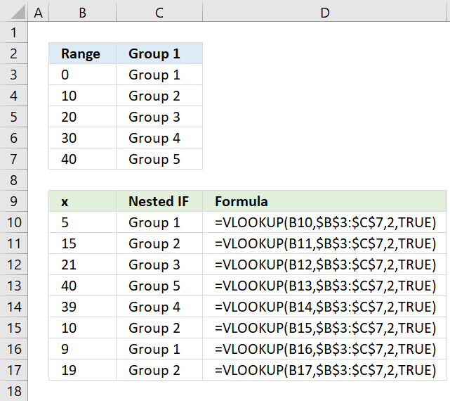
Imagine that you have 5 different groups, you now need to add six more nested IF statements. The formula grows considerably, however, the VLOOKUP function is really useful in this case.
The VLOOKUP lets you easily group numbers using a simple function instead of constructing a mega formula that is hard to follow and troubleshoot.
Need more groups? No, problem. Add groups to the first table and then adjust the cell reference in the second argument in the VLOOKUP function.
Note, the first table must have the first column sorted from small to large. Make sure you use TRUE in the fourth VLOOKUP argument. This means that it only needs an approximate match.
Read more about the VLOOKUP function.
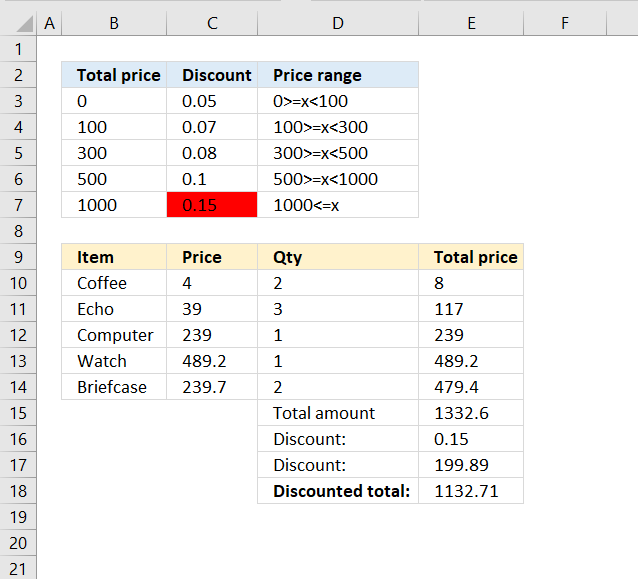
33.3. How to simplify nested IF functions based on conditions

These nested IF statements in cell C3 check if a value is equal to a condition and returns another value if True.
Nested IF function formula in cell C3:
You can use the VLOOKUP function in this case as well as an alternative to nested IF functions. You need to find an exact match in this case so change the fourth VLOOKUP argument to FALSE.
The simplified formula in cell C8:
The VLOOKUP function looks for the value in the first column (E8:F11) and returns the corresponding value in the second column. That is why I use 2 in the third VLOOKUP argument.
33.3.1 Explaining formula in cell C11
Step 1 - Build table

The table above defines the conditions and what value to return.
Step 2 - VLOOKUP function
The VLOOKUP function lets you search the leftmost column for a value and return another value on the same row in a column you specify.
VLOOKUP(lookup_value, table_array, col_index_num, [range_lookup])
lookup_value - A value.
table_array - The range you want to use, remember that the VLOOKUP function always looks in the leftmost column in your specified range.
col_index_num - The column number which contains the return value.
[range_lookup] - True or False. True - approximate match, the leftmost column must be in ascending order. False - Exact match.
Step 3 - Populate arguments
VLOOKUP(lookup_value, table_array, col_index_num, [range_lookup])
lookup_value - B8
table_array - $E$8:$F$11
col_index_num - 2
[range_lookup] - FALSE.
VLOOKUP(lookup_value, table_array, col_index_num, [range_lookup])
becomes
VLOOKUP(B8, $E$8:$F$11, 2, TRUE)
Step 4 - Evaluate VLOOKUP function
VLOOKUP(B8, $E$8:$F$11, 2, TRUE)
becomes
VLOOKUP("V", {"V", "Level 1";"D", "Level 2";"S", "Level 3";"T", "Level 4"}, 2, TRUE)
and returns "Level 1" in cell C8.
Recommended articles
Have you ever tried to build a formula to calculate discounts based on price? The VLOOKUP function is much easier […]
33.4. How to simplify nested IF functions based on date ranges

The above image demonstrates how to use multiple date ranges with a short and simple VLOOKUP function. A date range consists of two dates, since these date ranges are contiguous the end date also represents the start date for the next range.
Formula in cell C3:
The first cell range is between 1/1/2017 and 2/15/2017. The second cell range is between 3/1/2017 and 6/1/2017.
33.4.1 Explaining formula in cell C11
Excel dates are really not much different from numerical values, in fact, they are numerical values formatted as dates.
1 is 1/1/1900 and 1/1/2000 is 36526. We can use the same technique described in section 2 to extract the correct quarter.
Step 1 - Build a table

The table above defines the date ranges and what value to return. Note, that there are no gaps between the date ranges.
Step 2 - VLOOKUP function
The VLOOKUP function lets you search the leftmost column for a value and return another value on the same row in a column you specify.
VLOOKUP(lookup_value, table_array, col_index_num, [range_lookup])
lookup_value - A value.
table_array - The range you want to use, remember that the VLOOKUP function always looks in the leftmost column in your specified range.
col_index_num - The column number which contains the return value.
[range_lookup] - True or False. True - approximate match, the leftmost column must be in ascending order. False - Exact match.
Step 3 - Populate arguments
VLOOKUP(lookup_value, table_array, col_index_num, [range_lookup])
lookup_value - B3
table_array - $E$3:$F$6
col_index_num - 2
[range_lookup] - True.
VLOOKUP(lookup_value, table_array, col_index_num, [range_lookup])
becomes
VLOOKUP(B3, $E$3:$F$6, 2, TRUE)
Step 4 - Evaluate VLOOKUP function
VLOOKUP(B3, $E$3:$F$6, 2, TRUE)
becomes
=VLOOKUP(42795, {42736, "Quarter 1"; 42826, "Quarter 2"; 42917, "Quarter 3"; 43009, "Quarter 4"}, 2, TRUE)
and returns "Group 1" in cell C3.
33.5. Excel file
34. OR function

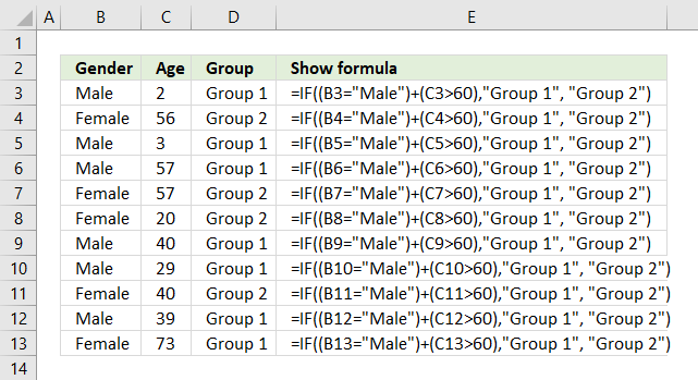
The formula above in cell D3 evaluates two different logical tests, if at least one of them is TRUE one thing happens, if all return FALSE another thing happens.
If a value in column B is equal to "Male" or a value on the same row in column C is above 60 the formula returns "Group 1", if none of these logical expressions return TRUE the formula returns "Group 2"
34.1 Explaining formula in cell D3
Step 1 - First condition
The equal sign is a logical operator, it lets you check if a value is equal to a condition. It returns a boolean value TRUE or FALSE.
B3="Male"
becomes
"Male"="Male"
and returns TRUE. Note that the comparison is not case sensitive, use the EXACT function if you want that functionality.
Step 2 - Second condition
The larger than sign is a also logical operator, it lets you check if a value is larger than a condition. It returns a boolean value TRUE or FALSE.
C3>60
becomes
2>60
and returns FALSE. 2 is not larger than 60.
Step 3 - Evaluate OR function
The OR function returns TRUE or FALSE based on a logical expression. It returns TRUE if at least one argument evaluates to TRUE, the OR function returns FALSE if all arguments return FALSE.
OR(B3="Male",C3>60)
becomes
OR(TRUE, FALSE)
and returns TRUE.
Step 4 - Evaluate IF function
The IF function returns one value if the logical test is TRUE and another value if the logical test is FALSE.
IF(logical_test, [value_if_true], [value_if_false])
IF(OR(B3="Male",C3>60),"Group 1", "Group 2")
becomes
IF(TRUE, "Group 1", "Group 2")
and returns "Group 1" in cell D3.
34.2 OR function or plus sign?
You can also wrap each logical expression with parentheses and use the + (plus sign) with the same functionality as the OR function.
Why wrap each logical expression? It determines the order of calculation, you want the comparisons to be calculated before you add the boolean values.
You now know what a plus sign means if you happen to see a formula with a plus sign. The advantage is a slightly smaller formula.
Explaining formula
Step 1 - First condition
The equal sign is a logical operator, it lets you check if a value is equal to a condition. It returns a boolean value TRUE or FALSE.
B3="Male"
becomes
"Male"="Male"
and returns TRUE.
Step 2 - Second condition
The larger than sign is a also logical operator, it lets you check if a value is larger than a condition. It returns a boolean value TRUE or FALSE.
C3>60
becomes
2>60
and returns FALSE. 2 is not larger than 60.
Step 3 - Add boolean values - OR logic
(B3="Male")+(C3>60)
becomes
TRUE + FALSE
and returns 1. 1 is the numerical equivalent to TRUE and 0 (zero) is FALSE.
Step 4 - Evaluate IF function
The IF function returns one value if the logical test is TRUE and another value if the logical test is FALSE.
IF(logical_test, [value_if_true], [value_if_false])
IF((B3="Male")+(C3>60),"Group 1", "Group 2")
becomes
IF(TRUE, "Group 1", "Group 2")
and returns "Group 1" in cell D3.
35. OR function - check if there is at least one number above a given value
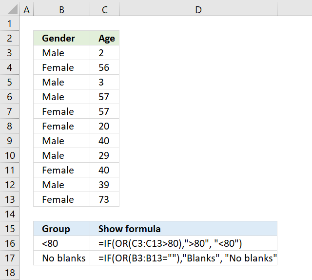
The array formula in cell B16 checks if there is a value larger than 80 in cell range C3:C13. You need to enter this as an array formula because you carry out a logical test to each cell in cell range C3:C13 and that logical test returns an array of boolean values.
The OR function then returns TRUE if at least one boolean value is TRUE in the array or else FALSE. The IF function returns <80 if there are no values above 80 and >80 if there is at least one value above 80 in cell range C3:C13.
Explaining formula in cell B16
Step 1 - Check if values in cell range are larger than 80
The larger than sign is a also logical operator, it lets you check if a value is larger than a condition. It returns a boolean value TRUE or FALSE.
C3:C13>80
Step 2 - Apply OR logic
The OR function returns TRUE or FALSE based on a logical expression. It returns TRUE if at least one argument evaluates to TRUE, the OR function returns FALSE if all arguments return FALSE.
OR(C3:C13>80)
Step 3 - Evaluate IF function
The IF function returns one value if the logical test is TRUE and another value if the logical test is FALSE.
IF(logical_test, [value_if_true], [value_if_false])
C3:C13>80
36. Blank value in a cell range
The array formula in cell B17 checks if there are any blank values in cell range B3:B13.
36.1 How to enter an array formula
To enter an array formula press and hold CTRL + SHIFT simultaneously, then press Enter once. Release all keys.
The formula bar now shows the formula enclosed with curly brackets telling you that you entered the formula successfully. Don't enter the curly brackets yourself.
36.2 Explaining formula
Step 1 - Check if cells are empty
The equal sign is a logical operator, it lets you check if a value is equal to a condition. It returns a boolean value TRUE or FALSE.
B3:B13=""
Step 2 - Apply Or logic
The OR function returns TRUE or FALSE based on a logical expression. It returns TRUE if at least one argument evaluates to TRUE, the OR function returns FALSE if all arguments return FALSE.
OR(B3:B13="")
Step 3 - Evaluate IF function
The IF function returns one value if the logical test is TRUE and another value if the logical test is FALSE.
IF(logical_test, [value_if_true], [value_if_false])
IF(OR(B3:B13=""),"Blanks", "No blanks")
37. Function not working
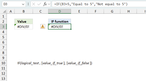
The IF function returns
- #VALUE! error if you provide an invalid logical test.
- #NAME? error if you misspell the function name.
- propagates errors, meaning that if the input contains an error (e.g., #VALUE!, #REF!, #DIV/0!), the function will return the same error.
37.1 Troubleshooting the error value
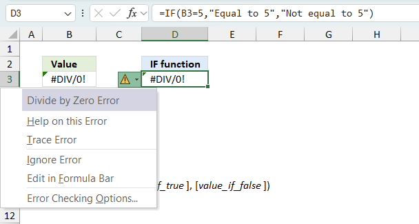
When you encounter an error value in a cell a warning symbol appears, displayed in the image above. Press with mouse on it to see a pop-up menu that lets you get more information about the error.
- The first line describes the error if you press with left mouse button on it.
- The second line opens a pane that explains the error in greater detail.
- The third line takes you to the "Evaluate Formula" tool, a dialog box appears allowing you to examine the formula in greater detail.
- This line lets you ignore the error value meaning the warning icon disappears, however, the error is still in the cell.
- The fifth line lets you edit the formula in the Formula bar.
- The sixth line opens the Excel settings so you can adjust the Error Checking Options.
Here are a few of the most common Excel errors you may encounter.
#NULL error - This error occurs most often if you by mistake use a space character in a formula where it shouldn't be. Excel interprets a space character as an intersection operator. If the ranges don't intersect an #NULL error is returned. The #NULL! error occurs when a formula attempts to calculate the intersection of two ranges that do not actually intersect. This can happen when the wrong range operator is used in the formula, or when the intersection operator (represented by a space character) is used between two ranges that do not overlap. To fix this error double check that the ranges referenced in the formula that use the intersection operator actually have cells in common.
#SPILL error - The #SPILL! error occurs only in version Excel 365 and is caused by a dynamic array being to large, meaning there are cells below and/or to the right that are not empty. This prevents the dynamic array formula expanding into new empty cells.
#DIV/0 error - This error happens if you try to divide a number by 0 (zero) or a value that equates to zero which is not possible mathematically.
#VALUE error - The #VALUE error occurs when a formula has a value that is of the wrong data type. Such as text where a number is expected or when dates are evaluated as text.
#REF error - The #REF error happens when a cell reference is invalid. This can happen if a cell is deleted that is referenced by a formula.
#NAME error - The #NAME error happens if you misspelled a function or a named range.
#NUM error - The #NUM error shows up when you try to use invalid numeric values in formulas, like square root of a negative number.
#N/A error - The #N/A error happens when a value is not available for a formula or found in a given cell range, for example in the VLOOKUP or MATCH functions.
#GETTING_DATA error - The #GETTING_DATA error shows while external sources are loading, this can indicate a delay in fetching the data or that the external source is unavailable right now.
37.2 The formula returns an unexpected value
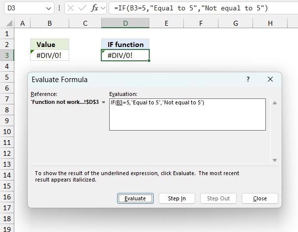
To understand why a formula returns an unexpected value we need to examine the calculations steps in detail. Luckily, Excel has a tool that is really handy in these situations. Here is how to troubleshoot a formula:
- Select the cell containing the formula you want to examine in detail.
- Go to tab “Formulas” on the ribbon.
- Press with left mouse button on "Evaluate Formula" button. A dialog box appears.
The formula appears in a white field inside the dialog box. Underlined expressions are calculations being processed in the next step. The italicized expression is the most recent result. The buttons at the bottom of the dialog box allows you to evaluate the formula in smaller calculations which you control. - Press with left mouse button on the "Evaluate" button located at the bottom of the dialog box to process the underlined expression.
- Repeat pressing the "Evaluate" button until you have seen all calculations step by step. This allows you to examine the formula in greater detail and hopefully find the culprit.
- Press "Close" button to dismiss the dialog box.
There is also another way to debug formulas using the function key F9. F9 is especially useful if you have a feeling that a specific part of the formula is the issue, this makes it faster than the "Evaluate Formula" tool since you don't need to go through all calculations to find the issue.
- Enter Edit mode: Double-press with left mouse button on the cell or press F2 to enter Edit mode for the formula.
- Select part of the formula: Highlight the specific part of the formula you want to evaluate. You can select and evaluate any part of the formula that could work as a standalone formula.
- Press F9: This will calculate and display the result of just that selected portion.
- Evaluate step-by-step: You can select and evaluate different parts of the formula to see intermediate results.
- Check for errors: This allows you to pinpoint which part of a complex formula may be causing an error.
The image above shows cell reference B3 converted to hard-coded value using the F9 key. The IF function requires non-error values which is not the case in this example. We have found what is wrong with the formula.
Tips!
- View actual values: Selecting a cell reference and pressing F9 will show the actual values in those cells.
- Exit safely: Press Esc to exit Edit mode without changing the formula. Don't press Enter, as that would replace the formula part with the calculated value.
- Full recalculation: Pressing F9 outside of Edit mode will recalculate all formulas in the workbook.
Remember to be careful not to accidentally overwrite parts of your formula when using F9. Always exit with Esc rather than Enter to preserve the original formula. However, if you make a mistake overwriting the formula it is not the end of the world. You can “undo” the action by pressing keyboard shortcut keys CTRL + z or pressing the “Undo” button
37.3 Other errors
Floating-point arithmetic may give inaccurate results in Excel - Article
Floating-point errors are usually very small, often beyond the 15th decimal place, and in most cases don't affect calculations significantly.
38. Get Excel *.xlsx file
'IF' function examples

First, let me explain the difference between unique values and unique distinct values, it is important you know the difference […]

This post explains how to lookup a value and return multiple values. No array formula required.

Array formulas allows you to do advanced calculations not possible with regular formulas.
Functions in 'Logical' category
The IF function function is one of 16 functions in the 'Logical' category.
Excel function categories
Excel categories
6 Responses to “How to use the IF function”
Leave a Reply
How to comment
How to add a formula to your comment
<code>Insert your formula here.</code>
Convert less than and larger than signs
Use html character entities instead of less than and larger than signs.
< becomes < and > becomes >
How to add VBA code to your comment
[vb 1="vbnet" language=","]
Put your VBA code here.
[/vb]
How to add a picture to your comment:
Upload picture to postimage.org or imgur
Paste image link to your comment.
[...] Interested in how the IF function works, read this post: IF function explained [...]
Hi Oscar
Thank you for your explanation and examples. I'd really appreciate it if you could you help me with this:
I'm trying to say, "if a cell from E2 to E89 contains 1, then sum the contents of the corresponding cell in D", ie. I only want to add D cell contents together if the corresponding E cell contains '1'.
=SUM(IF(E2:E89=1, D2:D89, 0))
Thank you!
Alison.
Another problem that is commonly solved by nestetd if is the intersection of two intervals.
Alternative formula:
IF A1 and A2 are the ends of the interval A
and B1 and B2 are the ends of the interval B
then intersection of interval A with interval B is:
=MAX(0,MIN(A2,B2)-MAX(B1,A1)+1)
Ciprian Stoian,
Thank you for your comment.
If interval A is 1 to 7 and interval B is 4 to 11 then the intersection is 4 to 7?
Ciprian Stoian
I now understand, your formula calculates if two intervals intersect or not.
The IF function is nicely explained. The examples used are varied covering different types of arguments and situations.