Lookup and return multiple values concatenated into one cell
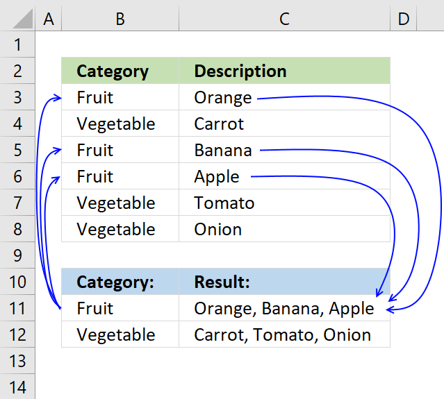
This article demonstrates how to find a value in a column and concatenate corresponding values on the same row. The picture above shows an array formula in cell F3 that looks for value "Fruit" in column B and concatenates corresponding values in column C.
The TEXTJOIN function introduced in Excel 2019 allows you to easily concatenate values, it also accepts arrays and nested functions.
However if your Excel version is missing the TEXTJOIN function you can use a User Defined Function, I have all instructions on how to do that in this post.
Table of Contents
- Lookup and return multiple values concatenated into one cell [Excel 2019]
- Lookup and return multiple values concatenated into one cell [UDF]
- Ignore duplicates [Excel 2019]
- Ignore duplicates [Excel 365]
- Ignore duplicates [UDF]
- Add a delimiting character between each value [UDF]
- Match if cell contains string [Array Formula]
- Match if cell contains string [User Defined Function]
- Searching for the first characters in a text string [Array Formula]
- Searching for the first characters in a text string [UDF]
- Lookup and return multiple dates concatenated into one cell [Array Formula]
- Lookup and return multiple dates concatenated into one cell [UDF]
- Lookup within a date range and return multiple values concatenated into one cell [Array Formula]
- Lookup within a date range and return multiple values concatenated into one cell [UDF]
- Split search string using a delimiting character and return multiple matching values concatenated into one cell (UDF)
- Split search string using a delimiting character and return multiple matching values concatenated into one cell - Excel 2019 formula (Link)
- Use multiple search values and return multiple matching values concatenated into one cell (UDF)
- Use multiple search values and return multiple matching values concatenated into one cell - Excel 2019 formula (Link)
- Concatenate cell values based on a condition - older Excel versions
1. Lookup and return multiple values concatenated into one cell [Excel 2019]

The image above demonstrates a formula that returns values concatenated based on a condition. The condition is specified in cell C10, if the condition is met in column B the corresponding value from column C on the same row is extracted and concatenated together.
For example, condition "Vegetable" is found in cells B4, B7, and B8. The corresponding values in cells C4, C7, and C8 are "Carrot", "Tomato", and "Onion". They are concatenated by the TEXTJOIN function that was introduced in Excel 2019.
Array formula in cell C11:
1.1 How to change the delimiting character
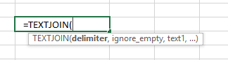
The first argument in the TEXTJOIN function lets you specify the delimiting character, I am using ", " in this example.
TEXTJOIN(delimiter, ignore_empty, text1, [text2], ...)
1.2 Watch a video where I explain the array formula
1.3 How to enter an array formula
Make sure you enter it as an array formula, follow this:
- Doublepress with left mouse button on cell C11
- Paste above formula to cell
- Press and hold CTRL + SHIFT simultaneously
- Press enter once
- Release all keys
If you did this the right way, the formula now has a beginning and ending curly bracket, like this:
{=TEXTJOIN(" ",TRUE,IF(A2='Vehicle applications'!$C$2:$C$13,'Vehicle applications'!$A$2:$A$13,""))}
Dont enter these characters yourself, they appear automatically if you follow the instructions above.
Then copy cell C2 and paste to cell range C3:C6.
1.4 Explaining formula in cell C11
Step 1 - Logical expression
The equal sign is a logical operator that allows you to compare value to value. The result is always a boolean value.
B11=B3:B8
returns {FALSE; TRUE; FALSE; FALSE; TRUE; TRUE}
Step 2 - Filter values
The IF function returns one value if the logical expression returns TRUE and another value if the logical expression returns FALSE.
The TEXTJOIN function can ignore empty values if we want to, we can configure the IF function to return empty values if the logical expression returns False.
IF(B11=B3:B8, C3:C8, "")
returns {""; "Carrot"; ""; ""; "Tomato"; "Onion"}
Step 3 - Filter values
The TEXTJOIN function allows you to combine text strings from multiple cell ranges and also use delimiting characters if you want.
TEXTJOIN(delimiter, ignore_empty, text1, [text2], ...)
TEXTJOIN(" ", TRUE, IF(B11=B3:B8, C3:C8, ""))
returns "Carrot, Tomato, Onion" in cell C11.
Here is another example:
Richard asks:
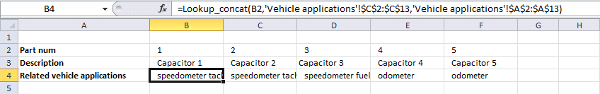
Looking for a formula that will take a part number from one column and go and look for all related vehicle applications per that part number and return the vehicle applications to a single cell related back to the part number.

Array formula in cell C2:
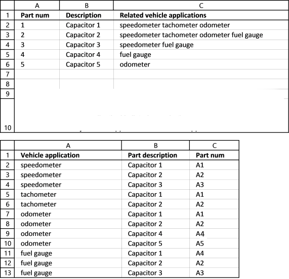
2. Lookup and return multiple values concatenated into one cell (UDF)

UPDATE: The solution below is for Excel versions that have the TEXTJOIN function missing.
User Defined Function in cell C2:
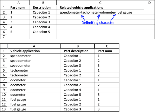
Picture below of worksheet "Vehicle applications".

Cell A1 (first picture above) contains "1" which is found in cells C2, C5, C7, and C11 (see picture above). The corresponding values on the same row from column A are "speedometer", "tachometer", "odometer, and "fuel gauge".
2.1 Watch a video where I demonstrate the UDF
2.2 User defined function Syntax
Lookup_concat(look_up_value, search_in_column, concatenate_values_in_column)
Looks for a value in a column and returns a value on the same row from a column you specify. If multiple values are found the corresponding values are concatenated into a single cell.
See the picture below.

2.3 VBA code
'Name user defined function and define parameters
Function Lookup_concat(Search_string As String, _
Search_in_col As Range, Return_val_col As Range)

'Dimension variables and declare data types
Dim i As Long
Dim result As String

'Iterate through each cell in search column
For i = 1 To Search_in_col.Count

'Check if cell is equal to search string
If Search_in_col.Cells(i, 1) = Search_string Then

'Concatenate corresponding value on the same row to the result variable
result = result & " "  Return_val_col.Cells(i, 1).Value
End If

'Continue with next cell
Next

'Return variable to worksheet
Lookup_concat = Trim(result)

End Function
2.4 Where to put the VBA code?
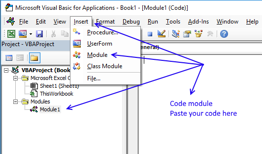
- Press Alt-F11 to open the Visual Basic Editor.
- Press the left mouse button on "Insert" located on the top menu, see the image above.
- Press left mouse button on "Module" on the Insert menu to create a new module in your workbook.
- Copy code above and paste to the code module, see the image above.
- Exit visual basic editor and return to Excel.
- Save your workbook as a *.xlsm file to keep the code attached to your workbook.
3. Ignore duplicates - Excel 2019

This example demonstrates how to ignore duplicate values in the output, it uses the TEXTJOIN function which was introduced in Excel 2019.
The picture below shows you "Carrot" found twice in the table but is only displayed once in cell C13. In other words, no duplicates are allowed in the output.
Array formula in cell C2:
Watch a video where I explain the formula
3.1 Explaining array formula in cell C13
Step 1 - Logical expression
The equal sign is a logical operator that lets you to compare value to value, the output is a boolean value.
In this case, the value in cell C12 is compared to all values in cell range B3:B10. The logical expression returns an array of boolean values.
C12=B3:B10
returns {FALSE; TRUE; FALSE; ... ; TRUE}.
Step 2 - Filter values
The IF function returns one value if the logical expression returns TRUE and another value if the logical expression returns FALSE.
IF(logical_test, [value_if_true], [value_if_false])
IF(C12=B3:B10, C3:C10, "")
returns {""; "Carrot"; ""; ... ; "Carrot"}.
Step 3 - Match values
The MATCH function returns the relative position of an item in an array or cell reference that matches a specified value in a specific order.
MATCH(lookup_value, lookup_array, [match_type])
MATCH(C3:C10, IF(C12=B3:B10, C3:C10, ""), 0)
returns {#N/A; 2; #N/A; #N/A; 5; 6; #N/A; 2}.
The MATCH function returns an error #N/A if the lookup_value is not found in the lookup_array, we will take care of this in the next step.
Step 4 - Remove errors
The IFERROR function lets you catch most errors in Excel formulas. We will replace the error value with an empty value.
IFERROR(value, value_if_error)
IFERROR(MATCH(C3:C10, IF(C12=B3:B10, C3:C10, ""), 0), "")
returns {""; 2; ""; ""; 5; 6; ""; 2}.
Step 5 - Create sequence
The ROW function calculates the row number based on a cell reference. We use a cell reference that points to a cell range instead of a single cell. This returns an array of numbers.
ROW(reference)
ROW(B3:B10)
returns {3; 4; 5; 6; 7; 8; 9; 10}.
Step 6 - Create a number sequence from 1 to n
MATCH(ROW(B3:B10), ROW(B3:B10))
returns {1; 2; 3; 4; 5; 6; 7; 8}.
Step 7 - Compare arrays
This step compares the arrays which are of the same size, both contain the same number of values.
This allows us to identify duplicate values, a number that doesn't match the sequence is a duplicate or a blank value.
MATCH(C3:C10, IF(C12=B3:B10, C3:C10, ""), 0), "")=MATCH(ROW(B3:B10), ROW(B3:B10))
returns {FALSE; TRUE; FALSE; .... ; FALSE}.
Step 8 - Filter unique distinct values
This step creates an array that contains only unique distinct values, in other words, no duplicates.
IF(IFERROR(MATCH(C3:C10, IF(C12=B3:B10, C3:C10, ""), 0), "")=MATCH(ROW(B3:B10), ROW(B3:B10)), C3:C10, "")
returns {""; "Carrot"; ""; ""; "Tomato"; "Onion"; ""; ""}.
Step 9 - Concatenate unique distinct values
The TEXTJOIN function allows you to combine text strings from multiple cell ranges and also use delimiting characters if you want.
TEXTJOIN(delimiter, ignore_empty, text1, [text2], ...)
TEXTJOIN(", ", TRUE, IF(IFERROR(MATCH(C3:C10, IF(C12=B3:B10, C3:C10, ""), 0), "")=MATCH(ROW(B3:B10), ROW(B3:B10)), C3:C10, ""))
returns "Carrot, Tomato, Onion" in cell C13.
4. Ignore duplicates - Excel 365

This formula is a dynamic array formula and works only in Excel 365, it is entered as a regular formula. Both the FILTER and UNIQUE functions are new functions in Excel 365.
These new functions make the formula considerably smaller and easier to understand.
Formula in cell C13:
4.1 Explaining formula in cell C13
Step 1 - Logical test
The equal sign is a logical operator that lets you compare value to value. The result is always a boolean value.
In this case, the value in cell C12 is compared to all values in cell range B3:B10. The logical expression returns an array of boolean values.
C12=B3:B10
returns {FALSE; TRUE; FALSE; ... ; TRUE}.
Step 2 - Filter values
The FILTER function lets you extract values/rows based on a condition or criteria.
FILTER(array, include, [if_empty])
FILTER(C3:C10,C12=B3:B10)
returns {"Carrot"; "Tomato"; "Onion"; "Carrot"}.
Step 3 - Create a unique distinct list
The UNIQUE function lets you extract both unique and unique distinct values and also comparing columns to columns or rows to rows.
UNIQUE(FILTER(C3:C10,C12=B3:B10))
returns {"Carrot";"Tomato";"Onion"}.
Step 4 - Concatenate values
The TEXTJOIN function allows you to combine text strings from multiple cell ranges and also use delimiting characters if you want.
TEXTJOIN(delimiter, ignore_empty, text1, [text2], ...)
TEXTJOIN(", ",TRUE,UNIQUE(FILTER(C3:C10,C12=B3:B10)))
returns "Carrot, Tomato, Onion".
5. Ignore duplicates (UDF)

The image above shows a User Defined Function in cell C2 that lookup and returns multiple concatenated unique distinct values.
Formula in cell C2:

The image above shows worksheet "Vehicle applications". The part number in cell A2 matches cells C2, C5, C7, C9, and C11. Cell C7 and C9 are duplicates, however, the UDF returns only one instance of each value.
5.1 Video
Watch a video where I explain how to use the UDF:
5.2 VBA code
You need to add two User Defined Functions to your workbook. They let you return unique distinct values concatenated into one cell, one UDF creates a unique distinct list and the other UDF concatenates the values.
'Name User Defined Function and define parameters
Function Lookup_concat(Search_string As String, _
Search_in_col As Range, Return_val_col As Range)

'Dimension variables and declare data types
Dim i As Long
Dim temp() As Variant
Dim result As String

'Create an array variable
ReDim temp(0)

'Iterate through all cells in the search range
For i = 1 To Search_in_col.Count

'Check if cell value equals search string
If Search_in_col.Cells(i, 1) = Search_string Then

'Add value to array if true
temp(UBound(temp)) = Return_val_col.Cells(i, 1).Value

'Add another container to array variable
ReDim Preserve temp(UBound(temp) + 1)
End If
Next

'Check if first value in array variable is not equal to nothing
If temp(0) <> "" Then

'Remove container from array variable
ReDim Preserve temp(UBound(temp) - 1)

'Start User defined function named Unique with parameter temp which contains values
Unique temp

'Iterate through array variable temp
For i = LBound(temp) To UBound(temp)

'Add each value in array variable temp to variable result and add a delimiting character
result = result & " " & temp(i)

'Continue with next value
Next i

'Remove leading and trailing blanks and then return string to worksheet
Lookup_concat = Trim(result)

'Continue here if first value in temp array is nothing
Else

'Return blank to worksheet, this avoids an error being returned when no values match the condition
Lookup_concat = ""
End If

End Function
The following UDF returns a unique distinct list
'Name user defined function and define parameter
Function Unique(tempArray As Variant)

'Dimension variables and declare data types
Dim coll As New Collection
Dim Value As Variant

'Enable error handling
On Error Resume Next

'Iterate through each value in tempArray
For Each Value In tempArray

'Check if value has more characters than 0 (zero), if so add string to collection coll
If Len(Value) <> 0 Then coll.Add Value, CStr(Value)

'Continue with next value
Next Value

'Disable error handling
On Error GoTo 0

'Clear array variable tempArray
ReDim tempArray(0)

'Iterate through each value stored in collection variable coll
For Each Value In coll

'Save value to array variable tempArray
tempArray(UBound(tempArray)) = Value

'Add another container to array variable tempArray
ReDim Preserve tempArray(UBound(tempArray) + 1)

'Continue with next value
Next Value

End Function
How to add vba code to your workbook
6. Change delimiting character (UDF)
This UDF lets you specify a delimiting character in the last argument.
Formula in cell C2:
The last argument in the User Defined Function lets you specify a delimiting string, it can be one character it can be many.
6.1 Watch a video where I explain the UDF
6.2 VBA Code
'Name user defined function and define parameters
Function Lookup_concat(Search_string As String, _
Search_in_col As Range, Return_val_col As Range, str As String)

'Dimension variables and declare data types
Dim i As Long
Dim result As String

'Iterate through each cell in search range
For i = 1 To Search_in_col.Count

'Check if cell value matches search string
If Search_in_col.Cells(i, 1) = Search_string Then

'Add value to result variable and delimting character specified in parameter str
result = result & str & Return_val_col.Cells(i, 1).Value
End If

'Continue with next cell
Next

'Check if the number of characters in result variable is larger than 0 (zero)
If Len(result) > 0 Then

'Remove last delmiting string
result = Right(result, Len(result) - Len(str))

'Return values to worksheet
Lookup_concat = Trim(result)

'Continue here if the number of characters in result variable is not larger than 0 (zero)
Else

'Return nothing to worksheet
Lookup_concat = ""
End If
End Function
How to add vba code to your workbook
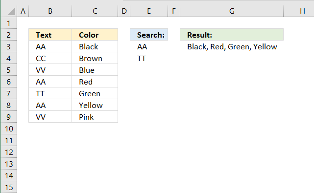
7. Match if cell contains string
This example demonstrates how to concatenate values if corresponding values on the same row contain a specific string.
The first image above shows the array formula in cell C2:
The way this works is that the formula in cell C2 checks if the value in cell A2 matches a string in cell range C2:C13. In other words, the whole cell is not required to match but a sub-string must.
Search string "1" is found in cell C2,C5 and C7 in the second image shown above, the corresponding values are "speedometer", "tachometer", and "odometer". Those values are returned to cell C2 shown in the first image above.
Watch a video where I explain the formula
7.1 Explaining array formula in cell C2
Step 1 - Search for string in cell range
The SEARCH function returns a number representing the position of character at which a specific text string is found reading left to right. It is not a case-sensitive search.
SEARCH(A2,'Vehicle applications'!$C$2:$C$13)
returns {2; #VALUE!; #VALUE!; ... ; #VALUE!}
Step 2 - Return adjacent value
The IF function returns one value if the logical test is TRUE and another value if the logical test is FALSE.
IF(logical_test, [value_if_true], [value_if_false])
IF(SEARCH(A2,'Vehicle applications'!$C$2:$C$13),'Vehicle applications'!$A$2:$A$13,"")
returns {"speedometer"; #VALUE!; ... ; #VALUE!}
Step 3 - Remove errors
The IFERROR function lets you catch most errors in Excel formulas.
IFERROR(value, value_if_error)
IFERROR(IF(SEARCH(A2,'Vehicle applications'!$C$2:$C$13),'Vehicle applications'!$A$2:$A$13,""),"")
returns {"speedometer"; ""; ""; .... ; ""}.
Step 4 - Concatenate values
The TEXTJOIN function allows you to combine text strings from multiple cell ranges and also use delimiting characters if you want.
TEXTJOIN(delimiter, ignore_empty, text1, [text2], ...)
TEXTJOIN(",",TRUE,IFERROR(IF(SEARCH(A2,'Vehicle applications'!$C$2:$C$13),'Vehicle applications'!$A$2:$A$13,""),""))
returns "speedometer, tachometer, odometer" in cell C2.
8. Match if cell contains string - User Defined Function

This example demonstrates a User Defined Function that matches cells that contain the search string and returns values from the same row concatenated, no duplicates are returned.
Formula in cell C2:

Cell A2 (first picture above) contains "1" which is found in cells C2, C5, and C7 (image above). The corresponding cells on the same row are concatenated and returned to cell C2 in the first picture above.
8.1 Video
For those of you that have an earlier Excel version. Watch this video where I explain how to use it:
8.2 VBA Code
'Name user defined function and define parameters
Function Lookup_concat(Search_string As String, _
Search_in_col As Range, Return_val_col As Range)

'Dimension variables and declare data types
Dim i As Long
Dim temp() As Variant
Dim result As String

'Create array variable
ReDim temp(0)

'Iterate through search range
For i = 1 To Search_in_col.Count

'Check if cell contains search string
If InStr(UCase(Search_in_col.Cells(i, 1)), UCase(Search_string)) Then

'Save cell value to array variable temp if line above is true
temp(UBound(temp)) = Return_val_col.Cells(i, 1).Value

'Add another container to array variable temp
ReDim Preserve temp(UBound(temp) + 1)
End If

'Continue with next cell
Next

'Check if first value in array variable temp is not equal to nothing
If temp(0) <> "" Then

'Remove last container in array variable temp
ReDim Preserve temp(UBound(temp) - 1)

'Iterate through values in array variable temp
For i = LBound(temp) To UBound(temp)

'Concatenate value to variable result and a delimiting character " "
result = result & " " & temp(i)

'Continue with next value
Next i

'Remove leading and trailing spaces and then return result variable to worksheet
Lookup_concat = Trim(result)

'Continue here if first value in array variable temp is equal to nothing
Else

'Return nothing to worksheet
Lookup_concat = ""
End If

End Function
How to add vba code to your workbook
9. Searching for the first characters in a text string
The formula and UDF demonstrated in the picture above look for a string that begins with the search string. If the search string is "a" it will match "ab", "ac" but not "ba". "ab" and "ac" begin with an "a".
If the search string is "ab" it will match "abc", "abz" but not "bca".
Array formula in cell C2:
Watch a video where I explain the formula
9.1 Explaining array formula in cell C2
Step 1 - Crop strings so they match search string length
The LEFT function extracts a specific number of characters always starting from the left.
LEFT(text, [num_chars])
LEFT('Vehicle applications'!$C$2:$C$13, LEN(A2)
returns {"a"; "b"; "c"; ... ; "c"}
Step 2 - Check if "a" is equal to values in array
The IF function returns one value if the logical expression returns TRUE and another value if the logical expression returns FALSE.
IF(logical_test, [value_if_true], [value_if_false])
IF(A2=LEFT('Vehicle applications'!$C$2:$C$13, LEN(A2)), 'Vehicle applications'!$A$2:$A$13, "")
returns {"speedometer"; ""; ""; ... ; ""}
Step 3 - Concatenate values
The TEXTJOIN function allows you to combine text strings from multiple cell ranges and also use delimiting characters if you want.
TEXTJOIN(delimiter, ignore_empty, text1, [text2], ...)
TEXTJOIN(",", TRUE, IF(A2=LEFT('Vehicle applications'!$C$2:$C$13, LEN(A2)), 'Vehicle applications'!$A$2:$A$13, ""))
returns "speedometer, tachometer, odometer, fuel gauge" in cell C2.
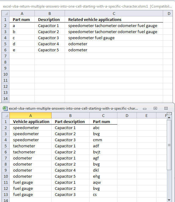
10. Searching for the first characters in a text string [UDF]

User Defined Function in cell C2:

The formula in cell C2, demonstrated in the first image above, concatenates values from column A if the corresponding value in column C (second image above) begins with the value specified in cell A2 (first image).
Cell C2, C5, C7, and C11 have values that begin with an "a", the formula in cell C2 returns these values "speedometer tachometer odometer fuel gauge" extracted from column A on the same rows as cells C2, C5, C7, and C11.
10.1 VBA code
'Name User defined Function and define parameters
Function Lookup_concat(Search_string As String, _
Search_in_col As Range, Return_val_col As Range)

'Dimension variables and declare data types
Dim i As Long
Dim result As String

'Iterate through all cells in search range
For i = 1 To Search_in_col.Count

'Check if cell begins with search string
If Left(Search_in_col.Cells(i, 1), Len(Search_string)) = Search_string Then

'Concatenate return value with variable result if search range value begins with search string
result = result & " " & Return_val_col.Cells(i, 1).Value
End If
Next

'Return variable result without leading and trailing space characters to worksheet
Lookup_concat = Trim(result)

End Function
How to add vba code to your workbook
11. Lookup and return multiple dates concatenated into one cell (formula)
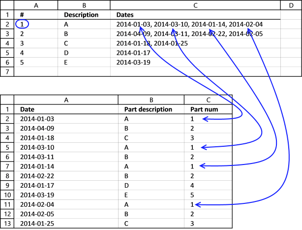
This example demonstrates a formula that concatenates dates based on a condition. The condition is specified in cell A2 shown in the first worksheet above.
The picture shows dates formatted in this order: YYYY-MM-DD, don't worry you can change this.
Array formula in cell C2:
Excel sees dates as numbers so they can be used in formulas and calculations, Jan 1, 1900 is 1, and June 7, 2017 is 42893. To concatenate dates and not numbers we need to use the TEXT function to convert numbers to dates.
Change date formatting to "MM/DD/YYYY" if you live in the United States.
Watch a video where I explain the formula
11.1 Explaining formula in cell C2
Step 1 - Format Excel date numbers to dates
The TEXT function converts a value to text in a specific number format, we will use this to convert Excel dates to dates.
TEXT(value, format_text)
TEXT('Vehicle applications'!$A$2:$A$13,"YYYY-MM-DD")
returns {"2014-01-03"; "2014-04-09"; "2014-01-18"; ... ; "2014-01-25"}
Step 2 - Check if "a" is equal to values in array
The IF function returns one value if the logical test is TRUE and another value if the logical test is FALSE.
IF(logical_test, [value_if_true], [value_if_false])
IF(A2='Vehicle applications'!$C$2:$C$13,TEXT('Vehicle applications'!$A$2:$A$13,"YYYY-MM-DD"),"")
returns {"2014-01-03";"";"";... ;""}
Step 3 - Concatenate values
The TEXTJOIN function allows you to combine text strings from multiple cell ranges and also use delimiting characters if you want.
TEXTJOIN(delimiter, ignore_empty, text1, [text2], ...)
TEXTJOIN(", ",TRUE,IF(A2='Vehicle applications'!$C$2:$C$13,TEXT('Vehicle applications'!$A$2:$A$13,"YYYY-MM-DD"),""))
returns "2014-01-03, 2014-03-10, 2014-01-14, 2014-02-04" in cell C2.
12. Lookup and return multiple dates concatenated into one cell [UDF]

This example demonstrates a User Defined Function that extracts and concatenates dates based on a condition applied to values in another column.
User Defined Function in cell C2:
The image below shows worksheet Vehicle applications.

The UDF concatenates dates from column A if values in column C on the same row match the condition specified in cell A2 (first image above).
12.1 VBA code
'Name User defined Function and define parameters
Function Lookup_concat(Search_string As String, _
Search_in_col As Range, Return_val_col As Range)

'Dimension variables and declare data types
Dim i As Long
Dim result As String

'Iterate through each cell in search range
For i = 1 To Search_in_col.Count

'Check if cell value matches search string
If Search_in_col.Cells(i, 1) = Search_string Then

'Add value to result variable and delimting character specified in parameter str
result = result & ", " & Return_val_col.Cells(i, 1).Value
End If
Next

'Remove delimiting characters and return string to worksheet
Lookup_concat = Right(result, Len(result) - 2)

End Function
How to add vba code to your workbook
13. Lookup within a date range and return multiple values concatenated into one cell
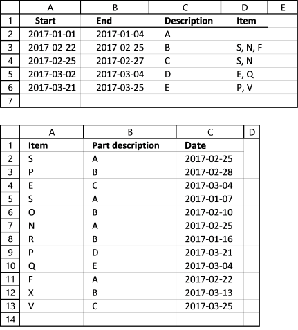
The following formula use a start and end date to filter dates in col C (table2) and return corresponding items on the same row in col A to cell D3.
Array formula in cell D3 (first worksheet above):
Watch a video where I explain the formula
13.1 Explaining formula in cell D3
Step 1 - Check which dates are larger than or equal to start date
The less than character and the equal sign are logical operators and check if dates are inside the date range. The output is an array of boolean values TRUE or FALSE.
A3<='Vehicle applications'!$C$2:$C$13
returns {TRUE; TRUE; TRUE; ... ; TRUE}.
Step 2 - Check which dates are smaller than or equal to start date
B3>='Vehicle applications'!$C$2:$C$13
returns {TRUE; FALSE; FALSE; ... ; FALSE}.
Step 3 - Multiply arrays - AND logic
Both conditions must be true for a date to be in a date range, this means we must apply AND logic meaning:
TRUE * TRUE = TRUE
TRUE * FALSE = FALSE
FALSE * TRUE = FALSE
FALSE * FALSE = FALSE
This requires us to multiply the arrays. Excel converts boolean values to their numerical equivalents when we multiply boolean values.
TRUE = 1 and FALSE = 0 (zero)
(A3<='Vehicle applications'!$C$2:$C$13) *(B3>='Vehicle applications'!$C$2:$C$13)
returns {1; 0; 0; ... ; 0}
Step 4 - Return value on same row as matching date
The IF function creates an array containing values from cell range A2:A13 worksheet "Vehicle applications" if the corresponding value in the array is TRUE or 1. If FALSE nothing "" is returned.
IF((A3<='Vehicle applications'!$C$2:$C$13) *(B3>='Vehicle applications'!$C$2:$C$13), 'Vehicle applications'!$A$2:$A$13, "")
returns {"S"; ""; ""; ... ; ""}
Step 5 - Concatenate values
The TEXTJOIN function allows you to combine text strings from multiple cell ranges and also use delimiting characters if you want.
TEXTJOIN(delimiter, ignore_empty, text1, [text2], ...)
TEXTJOIN(", ", TRUE, IF((A3<='Vehicle applications'!$C$2:$C$13) *(B3>='Vehicle applications'!$C$2:$C$13), 'Vehicle applications'!$A$2:$A$13, ""))
returns "S, N, F" in cell D3.
14. Lookup within a date range and return multiple values concatenated into one cell [UDF]

The UDF in cell D2 extracts and concatenates dates based on a date range specified in cells A2 and B2.
Formula in cell D2:
The following image show data on the second worksheet.

14.1 VBA code
'Name User Defined Function and define parameters
Function Lookup_concat(Search_Start As String, Search_End As String, _
Search_in_col As Range, Return_val_col As Range)

'Dimension variables and declare data types
Dim i As Long
Dim result As String

'Iterate through all cells in cearch range
For i = 1 To Search_in_col.Count

'Check if date is in date range
If Search_in_col.Cells(i, 1) <= Search_End And Search_in_col.Cells(i, 1) >= Search_Start Then

'Concatenate value from return range if date is in date range
result = result & Return_val_col.Cells(i, 1).Value & ", "
End If
Next

'Check if character length is larger than 0 (zero)
If Len(result) > 0 Then

'Remove last delimiting characters and return string to worksheet
Lookup_concat = Left(result, Len(result) - 2)

'Continue here date is not in date range
Else

'Return nothing to worksheet
Lookup_concat = ""
End If

End Function
How to add vba code to your workbook
15. Split search string using a delimiting character and return multiple matching values concatenated into one cell (UDF)

This UDF lets you use multiple search strings and fetch corresponding values concatenated to one cell.
Example, search string in cell A2 (table 1) is A+B, the search delimiting character is +. The UDF looks for both A and B in column A in table 2. Cell A2 and A3 matches A and B so the values from column B (Biology and Chemistry) are retrieved and concatenated to cell B2.
Formula in cell B2:
This is a User Defined Function so to use the above formula you need to first insert a few lines of code to your workbook.
15.1 VBA code
'Name User Defined Function and define parameters
Function Lookup_concat(Search_string As String, Search_del As String, _
Search_in_col As Range, Concat_del As String, Return_val_col As Range)

'Dimension variables and declare data types
Dim i As Long, j As Long
Dim result As String
Dim srchArr() As String

'Split search string based on delimting character and save to array variable srchArr
srchArr = Split(Search_string, Search_del)

'Iterate through search range
For i = 1 To Search_in_col.Count

'Iterate through values in array variable srchArr
For j = LBound(srchArr) To UBound(srchArr)

'Check if value equals value in search range
If Search_in_col.Cells(i, 1) = srchArr(j) Then

'Concatenate value to variable result and a delimtiing character
result = result & Return_val_col.Cells(i, 1).Value & Concat_del
End If
Next j
Next

'Remove laste delimting characters and return string to worksheet
Lookup_concat = Left(result, Len(result) - Len(Concat_del))
End Function
How to add vba code to your workbook
Remember to save your workbook as an *.xlsm file or your code is lost the next time you open your workbook.
17. Use multiple search values and return multiple matching values concatenated into one cell (UDF)
Formula in cell G3:
17.1 VBA Code
'Name User Defined Function and define parameters
Function Lookup_concat(Search_string As Range, Search_in_col As Range, Concat_del As String, Return_val_col As Range)

'Dimension variables and declare data types
Dim i As Long, j As Long
Dim result As String

'Iterate through search range
For i = 1 To Search_in_col.Count

    'Iterate through cells in parameter Search_string
    For Each Value In Search_string

        'Check if value is equal to cell in search range
        If Search_in_col.Cells(i, 1) = Value Then

            'Concatenate value to result and delimiting character
            result = result & Return_val_col.Cells(i, 1).Value & Concat_del
        End If
    Next Value
Next i

'Remove last delimiting characters and return string result to worksheet
Lookup_concat = Left(result, Len(result) - Len(Concat_del))
End Function
17.2 Get Excel *.xlsm file
Use multiple search values and return multiple matching values concatenated into one cell.xlsm
19. Concatenate cell values based on a condition

This article is for Excel users that don't have the latest Excel version or can't or don't want to use VBA code.
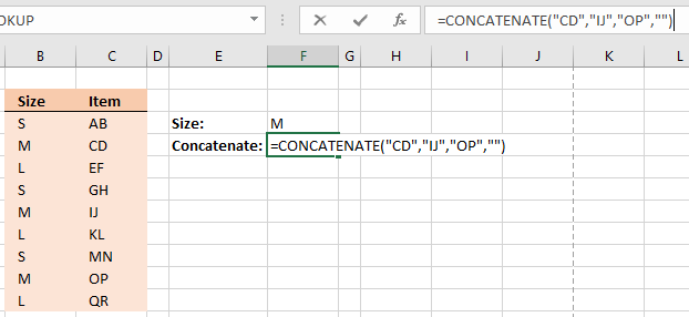
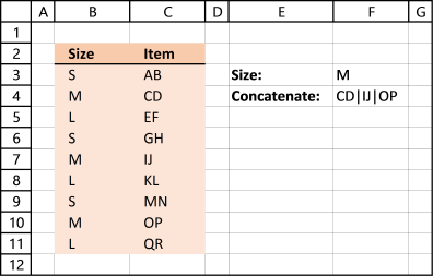
The image above shows you data in column B and C. I want to concatenate values on the same row as the condition specified in cell F2 which is in this case "M".
The corresponding values are "CD", "IJ" and "OP", in the picture above.
I highly recommend using the TEXTJOIN function if you use at least Excel 2019 or a later version.
For earlier versions than Excel 2019 use the user-defined function demonstrated here: Lookup and return multiple values concatenated into one cell
It is what the CONCATENATE function should have been from the beginning.
19.1. Create an array of values manually
- Copy (CTRL + c) this formula:
=TRANSPOSE(IF(B3:B11=F3,C3:C11,"")) - Double press with left mouse button on cell F4
- Paste (Ctrl + v) formula to cell F4
- Select the entire formula in the formula bar
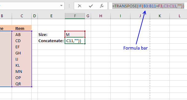
- Press Function key F9 and the formula is converted to an array of constants:
={"","CD","","","IJ","","","OP",""} - Delete the equal sign = in the formula bar and then press Enter
{"","CD","","","IJ","","","OP",""} - Select cell F4
19.1.1 Explaining formula
Step 1 - Logical expression
The equal sign is a logical operator that allows you to compare value to value. In this case, we are going to compare a single value to multiple values.
B3:B11=F3
returns {FALSE; TRUE; ... ; FALSE}.
Step 2 - IF function
The IF function returns one value if the logical test is TRUE and another value if the logical test is FALSE.
IF(B3:B11=F3,C3:C11,"")
returns {"";"CD";"";"";"IJ";"";"";"OP";""}.
Step 3 - TRANSPOSE function
The TRANSPOSE function allows you to convert a vertical range to a horizontal range, or vice versa. The CONCATENATE function needs the comma as a delimiting character to function properly.
TRANSPOSE(IF(B3:B11=F3,C3:C11,""))
returns {"", "CD", "", "", "IJ", "", "", "OP", ""}.
19.2. Delete blanks in the array
- I am now going to delete all empty characters in the array, press CTRL + H to open "Search and Replace" Dialog box
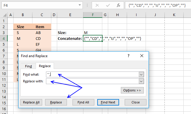
- Type in Find what: "", and nothing in Replace with:
- Press with mouse on "Replace" button
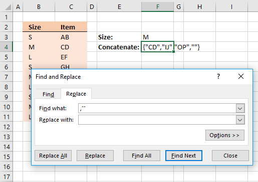
- Type in Find what: ,"" and nothing in Replace with:
- Press with left mouse button on "Replace" button once again.
- Press with left mouse button on Close button.
19.3. Concatenate all values in the array
The final thing to do is to use the concatenate function to add all values into one text string.
- Double press with left mouse button on cell F4
- Delete the curly brackets from the formula: {}
- Add this: =CONCATENATE(
- and then an ending parentheses )
- Press Enter

19.4. Add delimiting characters
Perhaps you want a delimiting character between values, right after you have converted the formula to an array of constants (step 5, above), do this:
- The array looks like this: ={"","CD","","","IJ","","","OP",""}
- Add an ampersand and then a delimiting character with quotation marks.
={"","CD","","","IJ","","","OP",""}&"|" - Select the formula and press function key F9, the formula now looks like this:
={"|","CD|","|","|","IJ|","|","|","OP|","|"}
The ampersand has added the delimiting character to all values in the array. - Continue with step 6 above. Tip! To delete empty values in array, Search and Replace with these values "|", and ,"|"
Concatenate category
More than 1300 Excel formulasExcel categories
293 Responses to “Lookup and return multiple values concatenated into one cell”
Leave a Reply
How to comment
How to add a formula to your comment
<code>Insert your formula here.</code>
Convert less than and larger than signs
Use html character entities instead of less than and larger than signs.
< becomes < and > becomes >
How to add VBA code to your comment
[vb 1="vbnet" language=","]
Put your VBA code here.
[/vb]
How to add a picture to your comment:
Upload picture to postimage.org or imgur
Paste image link to your comment.
Is there a way to list speedometer tachometer, etc... on separate lines in the same cell instead of separating them with a space? Similar to hitting the ALT+ENTER to create two lines of info in one cell like this:
cell C2
speedometer
tachometer
Tom,
Sure!
VBA code:
Function Lookup_concat(Search_string As String, _
Search_in_col As Range, Return_val_col As Range)
Dim i As Long
Dim result As String
For i = 1 To Search_in_col.Count
If Search_in_col.Cells(i, 1) = Search_string Then
result = result & " " & Return_val_col.Cells(i, 1).Value & Chr(10)
End If
Next
Lookup_concat = Trim(result)
End Function
Instructions:
Select cells.
Press CTRL + 1.
Press with left mouse button on tab "Alignment"
Enable "Wrap text"
Press with left mouse button on ok button!
Oscar,
I just left you a similar comment on another page. Is there a way to do this and put the results into new rows instead of the same cell?
1 Capacitor 1
2 Capacitor 2
Would become:
1 Capacitor 1 Speedometer
1 Capacitor 1 tachometer
1 Capacitor 1 odometer
1 Capacitor 1 fuel gauge
2 Capacitor 2 Speedometer
2 Capacitor 2 tachometer
... and so on
Thanks!
Peter
Hi Oscar,
Your macros is awesome!
A quick question though, if I need to search and return values in rows instead of columns, how can I edit the macro to reflect this? My interim fix was to transpose the entire table.
Thanks!
Cheers,
Faus
Oscar thank for the quick response. Is there a way to do this without UDF?
What I am trying to do is make an output matrix which has various wire types listed in column B4 thru B23 and terminating connector types listed across row C4 to AA4. I am trying to populate basically all of my open cells between C4 and AA23 with actual six digit part numbers. In some cases there are two six digit part numbers that must show up in the same cell. The data is being looked up in another tab in the spreadsheet with wire type in column C, part numbers in column B and connector type in column E. I also have a column called Standard flagged with a 1, 0 or black. What I am currently doing is using a combination of Index and Match in my output matrix that looks up a part number based on three criteria, wire type, connector type and a standard part (flagged with 1). If a row meets those three criteria the part number is grabbed and filled into the output matrix. I have that part working, but don't know how to list two part number in the same cell if that condition exists.
Is there a better way of doing this task?
Tom,
You could try to concatenate two formulas in a cell. See this page: https://excel.tips.net/Pages/T002788_Simulating_AltEnter_in_a_Formula.html
Thanks Oscar. Does the UDF stay with the file (embedded) if it is emailed and shared around the office or do you have to setup the VBA code on each individual's machine?
Tom,
The udf stays with the *.xls file.
Oscar thanks for this one. Saved me lot of time
Gonzo,
you are very welcome!
Oscar, I love this and am planning to use the code for a stock checking application. My Question is can it be modified to put the results on separate colums [in line with each search row]
Search Item Item1 Item2 Items 3
Ray, yes it can. But it would be easier to use this formula: How to return multiple values using vlookup in excel with a minor change.
How to create an array formula
Copy (Ctrl + c) and paste (Ctrl + v) array formula into formula bar.
Press and hold Ctrl + Shift.
Press Enter once.
Release all keys.
How to copy array formula
Select cell
Copy (Ctrl + c)
Select cell or cells to the right
Paste (Ctrl + v)
Hi Oscar
I want to use your above formula with a calendar in excel but I keep getting a #VALUE! error.
I have a data sheet that has data simular to this
1/2/2011 Red
1/3/2011 Blue
1/3/2011 Green
1/5/2011 Purple
I copied the lookup_concat udf and my function in column F5 of my calendar is...
=Lookup_concat(F4, Data!A4:A147, Data!B4:B147)
F4 is the field that has my date I was to search for.
Julie,
I am guessing the dates causes problems.
1. Select F4
2. Press Ctrl + 1
3. Press with left mouse button on Category: General
4. Remember the value
5. Press left mouse button on Cancel
Select the same date in range Data!A4:A147.
Repeat step 2 to 5.
Are the values the same?
How Excel Stores Dates And Times
Yes they are the same. I does work with vlookup but I want to be able to return multiple values.
This is my vlookup function in another cell and it does work. =VLOOKUP(D4,Data!A4:B378,2,FALSE)
Julie,
I have no idea!
Send me a workbook without sensitive data and I´ll see what I can do.
Wow Oscar, you rule! Searched the internet and beyond looking for this tiny fuction, thank you very much!
Bernard,
Thanks!
Hi Oscar - nice code you've got up here, and great explanation. This is close to what I need, but I'm trying to take multiple input values and output to one cell. I'm doing a skills inventory, where someone could have multiple skills like say Excel and Powerpoint. I'd like to be able to enter multiple numbers and return multiple values - got any tricks for that? Thanks!
Michael,
Yes, open attached file: excel-vba-search-for-multiple-values-and-return-multiple-values-into-one-cell.xls
Hi Oscar, your site had been a phenomenal help so far to me. I am interested in expanding the search multiple values/return multiple values to include multiple criteria
Would be entered something like this:
Lookup_Concat(Return_Col, Search_Col1, Range1, Search_Col2, Range2, Search Col 3, Range3)
What change(s) to the multiple value/multiple return would I make? Thanks! - A
Oscar - you make this look entirely too easy. I also came up with a way (with some help from a friend) where we changed the lookup key to text and used some string functions to get the desired result w/out VBA. This is more elegant, however. If you like I can post/send the file, I'm just not sure how to do that from this page. Thanks again! - Mike
Got the example file, but showed #NAME? error in column C under Related vehicle applications.
Looks like an error in the code?
I had the same problem. It turned out that I didnt have macros enabled in the trust center
a,
I opened the file and it works here.
Is there anyway to get it to ignore duplicates entries?
so that each 'vehicle application' is listed once in the 'related vehicle applications' no matter how many times it appears in the 'vehicle application' list?
Matt,
Yes, get example file:
excel-vba-return-multiple-unique-values-into-one-cell.xls
How would you integrate the multiple criteria lookup_concat function with the above mentioned functionality to remove duplicates?
Thank you Oscar
that has proved to be very useful
Hi Oscar thank you for your code it works well for me with a small exception. I have used your code shown to Tom (26th Jan 2011). When the code concatenates two or more text strings the text is placed on successive lines but there is always a ALT + ENTER character at the end of the text that adds an extra line below the last text string.
Is there any way to prevent the this last ALT + ENTER from being added?
Thank you for your help
Chris,
Search_in_col As Range, Return_val_col As Range)
Dim i As Long
Dim result As String
For i = 1 To Search_in_col.Count
If Search_in_col.Cells(i, 1) = Search_string Then
result = result & " " & Return_val_col.Cells(i, 1).Value & Chr(10)
End If
Next
result = Left(result, Len(result)-1)
Lookup_concat = Trim(result)
End Function
Oscar, Very Nifty, Thanks
Modified to insert commas & ampersand:
Function Lookup_concat(Search_string As String, _
Search_in_col As Range, Return_val_col As Range)
Dim i As Long
Dim n As Integer
Dim c As Integer
Dim result As String
For i = 1 To Search_in_col.Count
If Search_in_col.Cells(i, 1) = Search_string Then
n = n + 1
End If
Next
For i = 1 To Search_in_col.Count
If Search_in_col.Cells(i, 1) = Search_string Then
c = c + 1
Select Case c
Case 1
result = Return_val_col.Cells(i, 1).Value
Case n
result = result & " & " & _Return_val_col.Cells(i, 1).Value
Case Else
result = result & ", " & Return_val_col.Cells(i, 1).Value
End Select
End If
Next
Lookup_concat = Trim(result)
End Function
This is great. How do I make this UDF available for all my spreadsheets without having to inserting it into each spreadsheet?
This is so wonderful. Is there a way to add commas between each entry?
Vicki,
Function Lookup_concat(Search_string As String, _ Search_in_col As Range, Return_val_col As Range) Dim i As Long Dim result As String For i = 1 To Search_in_col.Count If Search_in_col.Cells(i, 1) = Search_string Then result = result & "," & Return_val_col.Cells(i, 1).Value End If Next result = Left(result, Len(result)-1) Lookup_concat = Trim(result) End FunctionHi, this works great with the comma though is it possible to not start the result with a comma as it appears to do but end with a comma in the result?
Was their ever a response to this? Is there a way to not start off with a comma but have any entries after the first be separated with a comma?
Hi Holly,
Try this.
Thanks,
Alex
_____________________________________________
Function Lookup_concat(Search_string As String, _
Search_in_col As Range, Return_val_col As Range)
Dim i As Long
Dim result As String
For i = 1 To Search_in_col.Count
If Search_in_col.Cells(i, 1) = Search_string Then
result = result & ", " & Return_val_col.Cells(i, 1).Value
End If
Next
result = Mid(result, 2, Len(Trim(result)) - 1)
Lookup_concat = Trim(result)
End Function
Alex,
That worked perfectly!! Thank you so much for your help!
Holly
Is there anyway to get this to work by adding in a third factor? I have a similar list with part numbers, but I only want to concatenate the products (or stores in my case) that have prices.
Rich,
Excel toolbox: Save your custom functions and macros in an Add-In
Thanks Oscar, I keep getting #VALUE! I believe this is happening because some of the search fields have #NAME errors. Any way to modify the script to ignore errors and continue looking?
Hi Oscar,
You are unbelievable with this! I have a question....
What if the return values from the function (Return_val_col) were integers and instead of listing all of the separate values in one cell, the function returned the sum of the values...
do you know how I could do that using the function that you created?
Naajia,
I attached both a vba and a formula solution. I do recommend using the formula.
https://www.get-digital-help.com/wp-content/uploads/2010/12/Naajia.xls
Oscar -- found this with a Google search, and it is EXACTLY what I needed. THANK YOU for your contributions here!!! Saved me a TON of time on a vital project.
Thank you Oscar.
Found this the same as Brad with Google search.
This very nice and clearly illustrated example helped me quite a bit.
Hello,
I was wondering if you could help me change the column look-up to a row based look-up. Instead of searching in one column I would like to search in 1 row for a certain number. Then display the results just as you have done.
Thank you.
Katherine
Oscar,
Like the rest, I'm thrilled to find your formula. Could it be modified to have a second (and maybe third) search column, kind of like a COUNTIFS() function would do?
Thanks,
Peter
Peter,
Did you figure out a way to set this up with multiple criteria?
Where I've put 17, just include the number of columns further away.
Option Explicit
Function Lookup_concat(Search_string As String, _
Search_in_col As Range, Return_val_col As Range)
Dim i As Long
Dim result As String
For i = 1 To Search_in_col.Count
If Search_in_col.Cells(i, 1) = Search_string Then
result = result & ", " & Return_val_col.Cells(i, 1).Value & " " & Return_val_col.Cells(i, 17).Value
End If
Next
Lookup_concat = Mid(result, 3)
End Function
Here is a link to an article I wrote in a "mini" blog I host which contains a UDF that I derived from this blog article's code but to which I added several additional optional arguments that provide some useful (I hope) flexibility when performing your lookup...
https://www.excelfox.com/forum/f22/lookup-value-concatenate-all-found-results-345/
Katherine,
Yes, see attached example file!
excel-vba-return-multiple-answers-into-one-cell-horizontal-lookup.xls
Like all the others I Googled to find what I needed and came upon this page. So thanks for the insight. Thanks Katherine for asking the same question that I was looking for. Thanks Oscar for providing the answer it worked great.
Rick Rothstein (MVP - Excel),
I tried your udf and all the optional arguments. It works great, I am sure it will be useful!
Hi Oscar,
Thanks very much for this UDF. Very useful. Is there a way that you know it can be used in a data validation list? I get an error if I use it and I read somewhere else that it's not possible to use UDF's. Basically I have a large table with fields 'country', 'operator', 'plan'. In another table I want to select a country, then in a second column get a list of (unique) operators available in that country and select one, and in a third column then select a plan based on the country operator choice in the other columns. Your UDF (with the appropriate separator and a little tweaking perhaps) would be ideal for that, but I need to find a way to use it in selection lists.
Thanks,
Mario.
Mario Hoek,
I think you will find these posts interesting:
https://www.get-digital-help.com/create-dependent-drop-down-lists-containing-unique-distinct-values-in-excel/
https://www.get-digital-help.com/dependent-data-validation-lists-in-multiple-rows/
Oscar,
First off, thanks so much for all your help. Your site has helped me many times.
My question stems off of Tom's question, and I've basically used the same code you've provided to Tom. My problem is, I have a range of a week (e.g. 5/7/12 - 5/13/12, 5/14/12 - 5/20/12, etc.) and from a list of individual dates, I have to determine if a date falls into that range, then it needs to return the corresponding text for each of those dates within the same cell (concatenated).
So if I have a range of 5/7/12 - 5/13/12, I need the macro to look at a list of dates, determine which of the dates fall between that range, and return the text in the adjacent column to that individual date.
Thanks again!
Jonah,
VBA Macro
Function Lookup_concat(SearchDate As String, _
StartDate As Range, EndDate As Range, Return_val_col As Range)
Dim i As Long
Dim result As String
For i = 1 To StartDate.Count
    If StartDate(i, 1) <= SearchDate Then
        If EndDate(i, 1) >= SearchDate Then
            result = result & " " & Return_val_col.Cells(i, 1).Value & Chr(10)
        End If
    End If
Next i
result = Left(result, Len(result) - 1)
Lookup_concat = Trim(result)
End Function
Get the Excel *.xslm file
Concatenate-values-within-matching-date-ranges1.xlsm
Oscar,
Thanks so much for replying. My output would actually need to look more like a concatenated form of column F.
Column B would actually be a non-concatenated search input (with one date for each text).
For example, given the date range from D2 to E2, the macro should look up which date in A2:A5 corresponds to that range, and return the concatenated form of each of the text.
See the excel file: https://docs.google.com/open?id=0B0B7Aw7pD4WCanJlMnlJbHpQRDQ
Thanks again!
Oscar,
Kindly disregard the last post. I've figured it out using your explanation on this page and other pages on your site.
I greatly appreciate the help you've so graciously given.
Hi Oscar
I am using your function Lookup_concat to fetch data from some other excel file. But I am facing a problem. If I use Vlookup (built-in excel function), then I get the result even if source file is closed. But Lookup_concat function only gives result if source file is opened, otherwise it gives #VALUE!
Pls help me here.
Thanks
Amit Gandhi
Amit Gandhi,
VBA does not support accessing information from closed workbooks.
Links:
Accessing ranges in closed workbooks in custom functions
INDIRECT and closed workbooks
Excel Automation: How to use an external link as an argument in a user-defined function?
Hi Oscar
I read your links provided, but i am unable to get the desired result, as I am not very much expert in VBA.
One link is suggesting to use ADO, other is suggesting to use HYPERLINK (When an Excel workbook is closed, it cannot be referenced by the INDIRECT function, however as Greg states this can be achieved via an acrimonious HYPERLINK function without having to resort to VBA/coding of any kind.)
Can you please help me how to modify LOOKUP_CONCAT function to get result from closed workbooks as well.
Amit Gandhi,
I would happily help you out but I have no clue.
Thanks Oscar for your valuable time.
Hi oscar
Thanks for your helpful website.I need to lookup in one column and return the results of two other columns.also I need to lookup in one column and return the results of two other column if the date in datecolumn in that row is equal to date in cell B2.I modified your vba code but i don't know it is correct or not beacuse when i put it in my spreadsheet it take a lot of time to calculate.and sometimes didn't work and return error value.
I need your comments.
here is my sample data:https://docs.google.com/open?id=0B6n9ww2vwHPMSFZwelNDRGt0Nmc
Hi Oscar,
Thanks for informative post. I need to lookup values from Column C (ticket #) based on Column A (Date) and Column B (Person). The look-up could return multiple values from column C (multiple tickets for a date). I need to concatenate multiple values in one cell of date –person matrix. UDF discussed here works but only problem is that it is not doing lookup on multiple columns. Can you please help?
Thanks in advance
Thank you for this - it's a brilliant, simple solution that works a treat.
Hi Oscar -
TO echo the question Peter posted in March - is there anyway to modify this formula and UDF so that it searches multiple criteria in 2 different columns?
This UDF is FANTASTIC!
Jen
I am on it.
Thanks!
Hi Oscar! Are you having any luck with this? I've looked everywhere for help with this and nothing...I'm counting on you!
Thanks!
Just discovered that this is case sensitive - I was confused that it wasn't finding things that other Excel functions (such as VLOOKUP) can find. How can I make it ignore the case of a letter? To force the source and the user input to be the same is not practical, unfortunately.
Ignore previous comment. To resolve the case sensitive issue, pop "Option Compare Text" on a line at the top of the module and searches will not be case sensitive.
Oscar, you are a life saver. I did have to change on line of code to get it to work for my needs.
From:
result = result & "," & Return_val_col.Cells(i, 1).Value
To:
result = Return_val_col.Cells(i, 1).Value & "," & result
Works fine now, but I one slight change would make it perfect:
Is there a way to make it only return UNIQUE values? Instead of:
207,207,205,206
It would say
207,205,206
I posted a link to a function I developed earlier in this thread which will allow you to do what you have asked for. Here is that link again...
https://www.excelfox.com/forum/f22/lookup-value-concatenate-all-found-results-345/
Rick,
Is your function able to search based on multiple criteria and return multiple values concatenated into one cell?
This is what I'm desperate to find an answer for!
Thanks,
It is a function, so you can call it for each of your search words and concatenate the results together (if you have a lot of search words, you may need to construct a loop to process them efficiently). If you want me to add additional functionality to my code, post the request against my mini-blog article over in my blog-site's forum location and I will attempt to comply there.
https://www.excelfox.com/forum/f22/lookup-value-concatenate-all-found-results-345/
Hi Thanks for this,
How would change search_string to lookup any value greater than 0?
Hi Oscar,
The code works great, thank you! I keep getting #VALUE for items that do not have a match.
I have a calendar and some things are in progress, planned, etc. If for a day, there are no planned items, I want it to be blank in the planned column...can't seem to figure it out. Can solve it with IF(ISERROR), but would like to incorporate into UDF, and can't seem to figure it out.
Many thanks!
Back awhile ago in the comment section for this blog article, I posted a link to an alternative UDF to the one Oscar posted which provided some extra functionality. One of the things my UDF does is return the empty string ("") when the text being searched for cannot be found. Here is a link to my mini-blog article where I posted that alternative UDF code for your consideration...
https://www.excelfox.com/forum/f22/lookup-value-concatenate-all-found-results-345/
thanks!
Christy,
I tried the udf for items that don´t have a match and I get a blank cell in those cases. I am using excel 2010.
I am using Excel 2007. The code Rick referred to worked, but it makes Excel hang way too much.
Yes, I have found the same issue.
I am having the problem that this code only looks in formulas not values, whereas Rick's does look in the values and finds what is needed... however, I can't use his code as it just crashed the computer because of the large amounts of data I am dealing with! :(
Is there any way to adapt this module to look in values?
Hi I was wondering if instead of showing the results separated by a space in on cell, I could make the results added to eachother in one cell.
I'm trying to lookup more than one value (number,e.g.prices)but show it added to all the other results.
thanks in advance
@Ralfy - I am having trouble visualizing what you are asking for... can you post a small sample of data and show us what you want that data to look like after it has been processed?
I have a small table where the data get imputed it has a row for the name of each person in charge of getting sales and credits for a 4 hrs period (4 to 5 rows) the columns are: name of person, amount of credits, $ sale up to that time, sale for the person ( has a formula that takes away what anyone before makes to know what this person sale is, credit productivity (sale/credits)
Then there is worksheet for each person where it looks up the sales, credit and productivity for that person for the day.
All of that I already have set up using vlookup. My issue is when the data sheet has more than one entry per day per day. I would like the lookup function to recognize more than one entry and add them up then insert to the persons worksheet.
Hope that helps,
Thank you in advance for your help, I hope to resolve this issue soon.I have a file, Cells A1:A50 have multiple e-mail addresses separated by ";". On Column B, I have a list of 1,000 e-mail addresses, each cell on column B has only one address. What I am trying to get to, is on Column C, to see which e-mails from cell A1 are found in the entire column B. Then which e-mails from cell A2 are found in the entire column B, and so on. If I need to send a spreadsheet please let me know. Thank you for your help.
Give this a try... put the following formula in C1 and copy it down:
=IF(COUNTIF(A:A,"*"&B1&"*"),"X","")
Ha, dummy me, I was thinking it too complicated, with Index and Match formulas. Should have thought the other way around, many thanks for your help.
Alright, here is the next step on this. Now that I can find which individual e-mail address from Column A is listed in the entire column B, I need to do a look-up and give me the corresponding category listed on column C.
Column A Column B Column C
e-mail1 e-mail1;e-mail2;e-mail4 CatA
e-mail2 e-mail3;e-mail6;e-mail7 CatB
How would I go about finding which value from Column A, is listed in Column B and then list it's corresponding value from column C?
Thank you in advance for your help with this.
Samsam,
e-mail1;e-mail2;e-mail4
What is this? Three emails in the first cell in column B or where are they entered?
Correct, Column A cells have individual addresses that are listed somewhere in the multitude of e-mails from Column B, which then have a corresponding category in column C. So while column A lists only 1 e-mail per cell, Column B cells have anywhere from 2 to 10 e-mail addressed in one cell. Then column C shows the category in which those e-mails belong.
SamSam,
I moved cell range B1:C6 to C1:D6. The formula in cell B1: =INDEX($D$1:$D$6,MATCH(A1,$C$1:$C$6,0))
Hi Oscar,
I've been trying to find the solution for my lookup problem for a while now and you seem like the right person to ask... Your lookup code works great (thanks) but I need to do two or three lookups within identified matching records... in other words:
Sheet 1 - 'File data'
1. client name
2. filename
3. file date create
Sheet 2 - 'Client data'
1. client name
2. client ID
3. service start date
4. service end date
I need to map correct client ID based on lookup by client name and then based on finding which service date range does client file created date fit into.
So I need to:
1. First search - Identify Client records with matching name
2. Second search - Within that range, I need to find fitting date range.
Your lookups are great when I search entire sheets but I need to do second seach based on subset of data.
Any help will be much appreciated.
Thanks!
Nena
Nena,
read this:
Search a table and use the returning value to search another table
Thanks Oscar,
regards,
Nena
[...] tableFiled in Dates, Excel, Search/Lookup on Sep.12, 2012. Email This article to a Friend Nena asks:Hi Oscar,I've been trying to find the solution for my lookup problem for a while now and you seem [...]
Thanks for posting very nice and effective UDF.
I had to change one line of code to get it to work for my needs.
From:
result = result & " " & Return_val_col.Cells(i, 1).Value
To:
result = result & "," & Return_val_col.Cells(i, 1).Value
but cannot omit last comma from the returned value. Any help in this respect will be highly appreciated. Thanks in advance.
sorry again after changing one line return value display like :
10, 12, 10,
but I want to omit last comma which will return like :
10, 12, 10
Thanks in advance
You get a **trailing** comma with that code line, not a LEADING comma??? You should double-check that as that code line can only produce a leading comma. And the way to get rid of it is by changing the last line of code from this...
Lookup_concat = Trim(result)
to this...
Lookup_concat = Mid(result, 2)
I know the number of comments for this article are quite long, so you may have missed the link I posted to a function I developed which extends the functionality of Oscar's UDF by adding additional options, so you might want to check it out here...
https://www.excelfox.com/forum/f22/lookup-value-concatenate-all-found-results-345/
Hi Oscar...this is a very interesting function and helped me a lot so far.
My file though is a bit more complicated..
I have multiple info in one cell separated with ";" (example AD1; AD2; AD3) lets say that these are servers (File name SERVERS) and in each server I have multiple applications. I have now another file that has all the applications per server per line in excel (each line has one server one application. File name: APPS).
I want starting from the file SERVERS to look up the servers that are in one cell find them in the second file APPS and bring all the applications also in one cell in the file SERVERS.
Any ideas here?
Thanks in advance
C
Chrisa,
see this post:
Lookup multiple values in one cell (vba)
Hi Oscar
the module seems to be looking in formulas by default rather then in values, which means it does not find any of the data in my fields (as they are all generated by concatenate formulas!)
You don't happen to have a fix for this by any chance???
Many thanks for your help
F
Hello again Oscar,
I just realised that the UDF does look in values... but it does not work on my sheet that contains xml data... it just returns #value
Hi Oscar,
I used your code for the option explicit fuction lookup_concat as well as the function unique. My problem lies in when i incorporate that into a nested formula:
=IF(D5"PO",Lookup_concat(B5,$B$2:$B$5000,$F$2:$F$5000),F5)
the formula works perfectly in the cells, but once i put that into the vba it gets stuck in an eternal loop and goes from
For i = 1 To Search_in_col.Count
  If Search_in_col.Cells(i, 1) = Search_string Then
    temp(UBound(temp)) = Return_val_col.Cells(i, 1).Value
    ReDim Preserve temp(UBound(temp) + 1)
  End If
Next
please help me.
my formula was supposed to read:
Valerie,
I tried a nested formula and it works here (excel 2010).
ok, so I realized that when I was watching my macro run step by step using F8 it appeared to be stuck in that loop once I hit your function. Once I just ran the macro (including your function) it worked perfectly. thank you for checking that. Do you have a place where I could continue to ask you questions with excel unrelated to this function?
Thank you so much again for your help.
valerie,
Do you have a place where I could continue to ask you questions with excel unrelated to this function?
No, most people search my site for answers. If they can´t find what they are looking for, they ask questions in blog posts.
I have a similar problem, but am finding that to search within vs for an exact value is causing the CONCAT formula to not work? Trying to look for value D2 withing column 2 of a Table1, then to return all values in column 3 of the table. Don't care if there are commas separating them, etc. Forumla only seems to work if it looks for an exact match. How do I change the following?
=Lookup_concat(D2&"*",'Table1'!B2:B7,'Table1'!C2:C8)
What am i doing wrong? The formula is returning nothing each time, though not getting any error??
Thanks in advance...
Additional question on this: the formula also does not seem to allow me to use named ranges vs selecting the range each time. Is there a way to update the formula to allow for named ranges?
Thanks...
Hi Oscar,
you are unbelievable! THANK YOU SO MUCH for all the answers!
[...] Chrisa asks: [...]
Hi Oscar.. Is there any way to use VLOOKUP for multiple criteria and Ido not want to use CVS... thanks in advance...
Kamran Mumtaz,
I read your question:
https://www.mrexcel.com/forum/excel-questions/682187-sumifs-unique-multiple-search.html#post3379273
This is the post you are looking for:
https://www.get-digital-help.com/automatically-filter-unique-row-records-from-multiple-columns/
Is there any way to use VLOOKUP for multiple criteria and I do not want to use CVS
I assume you don´t want to use CSE? (Ctrl + Shft + Enter) No, not to my knowledge.
Why did not you reply if you saw the question on Mrexcel board...? Many thanks for your help...
This is the formula given by Aladin Akyurek without (CSE)...
=INDEX(Sheet3!$B$2:$B$65,
MATCH(1,INDEX((Sheet3!$C$2:$C$65=E$1)*
(Sheet3!$A$2:$A$65=$A3),0,1),0))
Kamran Mumtaz,
Why did not you reply if you saw the question on Mrexcel board...?
A trackback is created when someone links to my website. That´s how I discovered your thread.
This is the formula given by Aladin Akyurek without (CSE)...
That formula is so interesting that I made this post:
No more array formulas?
Hi Oscar I have a list of numbers like
923005054609
913005054609
923005054609
933005054609
923005054609
993005054609
953005054609
923005054609
923005054609
993005054609
923005054609
973005054609
923005054609
923005054609
I do not want those numbers which starts 92... hope I am making sense...
Thanks in advance
Kamran Mumtaz,
Array formula in cell C4:
=INDEX($A$1:$A$14, SMALL(IF(LEFT($A$1:$A$14, 2)*1=$D$1, MATCH(ROW($A$1:$A$14), ROW($A$1:$A$14)), ""),ROW(A1)))
Formula in cell D4:
=INDEX($A$1:$A$14, SMALL(INDEX((LEFT($A$1:$A$14, 2)*1=$D$1)*(MATCH(ROW($A$1:$A$14), ROW($A$1:$A$14)))+((LEFT($A$1:$A$14, 2)*1)<>$D$1)*1048577, 0, 0), ROW(A1)))
Get the Excel file
Kamran-Mumtaz.xlsx
HI Oscar thanks for the formula but I want the numbers which do not start from 92...
Hey I made a little change in the formula and got the desired result
=IFERROR(INDEX($A$1:$A$14,SMALL(IF(LEFT($A$1:$A$14,2)*1$D$1,MATCH(ROW($A$1:$A$14),ROW($A$1:$A$14)),""),ROW(A1))),"")
Thanks a lot man... :)
Kamran Mumtaz,
I am sorry!
=INDEX($A$1:$A$14, SMALL(IF(LEFT($A$1:$A$14, 2)*1<>$D$1, MATCH(ROW($A$1:$A$14), ROW($A$1:$A$14)), ""),ROW(A1)))
[...] Mumtaz asked: Is there any way to use VLOOKUP for multiple criteria and I do not want to use [...]
I love this function, but know very little about VBA. Can anyone suggest a way to tweak the code a bit so that the return results are delimited with a semicolon and a space, rather than just a space?
Thanks!
Elizabeth,
Function Lookup_concat(Search_string As String, _ Search_in_col As Range, Return_val_col As Range) Dim i As Long Dim result As String For i = 1 To Search_in_col.Count If Search_in_col.Cells(i, 1) = Search_string Then result = result & "; " & Return_val_col.Cells(i, 1).Value End If Next Lookup_concat = Trim(result) End FunctionHello Oscar,
thanks for your code , i use it for a file for same searching values and it Work fine.
all the searched data are numbers :
56|55|40|63|....
for exameple i only wana one value that is : < or = a value of an other cell ( 57) in this case i only get : 56 .
could you please give me an edit code.
thanks in advance
Hey Oscar,
This function looks like it's going to do exactly what I need it to do, however when I use it I get in my list I get #VALUE. I believe it's because the returned values are multiple email addresses ([email protected]). Is there anyway this would work with email addresses?
Joe,
This function looks like it's going to do exactly what I need it to do, however when I use it I get in my list I get #VALUE.
I am not sure whats wrong, maybe you don´t use absolute cell references in the function?
I believe it's because the returned values are multiple email addresses ([email protected]). Is there anyway this would work with email addresses?
I am sure it works with email adresses and duplicate email adresses.
Oscar et al., thank you for this on-going forum. It has been incredibly helpful! I have (what I hope to be) a simple question. I modified one of the posted UDFs so that the multiple outputs (in this case, character strings) are displayed in a single cell, with each character string led by a bullet and followed by a hard return (i.e., ALT-Enter). I'm using the following code:
Function LOOKUP_CONCAT(Search_string As String, _
Search_in_col As Range, Return_val_col As Range)
Dim i As Long
Dim result As String
For i = 1 To Search_in_col.Count
If Search_in_col.Cells(i, 1) = Search_string Then
result = result & "• " & Return_val_col.Cells(i, 1).Value & vbLf
End If
Next
result = Left(result, Len(result) - 1)
LOOKUP_CONCAT = Trim(result)
End Function
The problem is that if the originating cell is empty, a bullet still appears. Is there a way I can modify the above code to eliminate the bullets for empty cells?
Thanks in advance for help!
Amanda,
try this:
Function LOOKUP_CONCAT(Search_string As String, _ Search_in_col As Range, Return_val_col As Range) Dim i As Long Dim result As String For i = 1 To Search_in_col.Count If Search_in_col.Cells(i, 1) = Search_string And Return_val_col.Cells(i, 1).Value <> "" Then result = result & "• " & Return_val_col.Cells(i, 1).Value & vbLf End If Next result = Left(result, Len(result) - 1) LOOKUP_CONCAT = Trim(result) End FunctionOscar,
Thank you for your quick response! The above code is sooo close... Instead of bullets, the blank cells now report "#VALUE!". Preferably, the blank cells would just be empty, but perhaps I can play around with the formula a bit.
All the best,
Amanda
Amanda,
Function LOOKUP_CONCAT1(Search_string As String, _ Search_in_col As Range, Return_val_col As Range) Dim i As Long Dim result As String For i = 1 To Search_in_col.Count If Search_in_col.Cells(i, 1) = Search_string And Return_val_col.Cells(i, 1).Value <> "" Then result = result & "• " & Return_val_col.Cells(i, 1).Value & vbLf End If Next If Len(result) <> 0 Then result = Left(result, Len(result) - 1) LOOKUP_CONCAT1 = Trim(result) Else LOOKUP_CONCAT1 = "" End If End FunctionJust in case I can save someone else a bit of time:
I used an IF function in combination with IFERROR to force Excel to report blank cells. For example:
IF((IFERROR((LOOKUP_CONCAT(A30,Database!A29:A617,Database!O29:O617)),"None"))="None","",(LOOKUP_CONCAT(A30,Database!A29:A617,Database!O29:O617)))
Hope that helps!
Thanks again!
Amanda
Hi Oscar. Thank you so much for sharing your extensive knowledge with us. I have a question. I am using that function that you gave for adding the values of the cells that I lookup .... =SUMPRODUCT((I5=C4:C32)*D4:D32)(Combined with the vba).... But I also have a need to find the average of those cells. Do you have a formula for that?
Thanks, Carla
Carla,
I don´t understand, can you explain in greater detail?
Hi Oscar,
This formula seems to work down a column, but I can't get it to work across rows. How would you amend the basic formula at the top so that it worked to compare 2 rows?
Thank you for sharing your knowledge. This is extremely helpful.
Eric,
I am not sure I understand.
Is this what you are looking for?
Hi Oscar,
I have a big excel file (around 22000 rows and 20 columns). Below I have tried to represent it in simplified way. Left hand side is my raw data and Right hand side is my desired output. If you can help me do this using functions (no vba code) that would be great. Please note all data is text.
I tried to upload the image but, does not look like it worked. Let me know how this can be resolved.
Nilesh,
use this contact form:
https://www.get-digital-help.com/excel-consulting/
Thanks Oscar.. I made a similar code to make it work like vlookup
Function SingleCellExtract(Lookupvalue As String, LookupRange As Range, ColumnNumber As Integer)
Dim i As Long
Dim Result As String
For i = 1 To LookupRange.Columns(1).Cells.Count
If LookupRange.Cells(i, 1) = Lookupvalue Then
Result = Result & " " & LookupRange.Cells(i, ColumnNumber) & ","
End If
Next i
SingleCellExtract = Left(Result, Len(Result) - 1)
End Function
Thanks for the cues I got from here
Sumit Bansal,
thanks for sharing!
Hi Oscar,
This has been a great help to me. I'm trying to get it to do one thing that I can't figure out though. For my application, almost all the lookup values are "1". I do however have a few instances where the lookup value could be 2 or 3. Is it possible to to use a range, e.g. 1-5 for my lookup value? Thank you.
Will,
Function Lookup_concat(Search_string1 As String, Search_string2 As String, _
  Search_in_col As Range, Return_val_col As Range)

Dim i As Long
Dim result As String

For i = 1 To Search_in_col.Count
  If Search_in_col.Cells(i, 1) <= Search_string2 And Search_in_col.Cells(i, 1) >= Search_string1 Then
    result = result & " " & Return_val_col.Cells(i, 1).Value
  End If
Next

Lookup_concat = Trim(result)

End Function
Get the Excel *.xls file
https://www.get-digital-help.com/wp-content/uploads/2010/12/excel-vba-return-multiple-answers-into-one-cell-using-a-search-range1.xls
Oscar,
its really great and helpful function will save lots of my time... Thanks
Had an query, i want to use this function within my macro by calling it, How can i do define 'Search_string', 'Search_in_col', 'Return_val_col' as an input and run this function cell by cell?
Thanks again...
Got it no need to reply... thank-you... thank-you very much.. god Bless u.
Oscar,
I love the code but I actually need to return multiple values meeting multiple criteria. (I think this is what Jen was looking for)
E.g.
If columnA=X AND columnB=Y then return columnC values concatenated into single cell.
Thanks
Still unclaer as to how I would achieve this.... if anyone could enlighten me I would be extremely grateful!
This is what I have at the moment
Function Lookup_concat(Search_string As String, _
  Search_in_col As Range, Return_val_col As Range)
Dim i As Long
Dim result As String
For i = 1 To Search_in_col.Count
  If Search_in_col.Cells(i, 1) = Search_string Then
    result = result & " " & Return_val_col.Cells(i, 1).Value
  End If
Next
Lookup_concat = Trim(result)
End Function
But I need an additional logical test in there...
E.g. If columnA=X AND columnB=Y then return columnC values concatenated into single cell.
Thanks
Adam,
try this:
Function Lookup_concat(Search_stringA As String, Search_in_colA As Range, _
Search_stringB As String, Search_in_colB As Range, Return_val_col As Range)

Dim i As Long
Dim result As String

For i = 1 To Search_in_colA.Count
    If Search_in_colA.Cells(i, 1) = Search_stringA And _
    Search_in_colB.Cells(i, 1) = Search_stringB Then
        result = result & " " & Return_val_col.Cells(i, 1).Value
    End If
Next i

Lookup_concat = Trim(result)

End Function
Get the Excel *.xlsm file
excel-vba-return-multiple-answers-into-one-cell-v3.xlsm
Amazing! Thank you!
[…] are some near solutions that I found but they consolidate the column data and not the row data. https://www.get-digital-help.com/excel-udf-lookup-and-return-multiple-values-concatenated-… https://www.ozgrid.com/forum/showthread.php?t=94895&p=445111#post445111 […]
Works great !!!
Just what i was looking for. Clean and simple.
Mike,
Thanks!
I cannot get the UDF to work properly within my file for the life of me. I need the values to populate with the project name on a project timeline chart based off the project schedule. Similar to the post on May 25, 2012 but it does not work in my sheet. It is not recognizing the date range and multiple values.
Here is what I am trying to do:
start date col B; project name col C;
timeline chart
beginning date col G; end date col H
I need the project names which will populate col I based off the start date of the project. Multiple dates should be concatenated to the proper month range in col I
Basically, if i have three projects starting on any date in January the project names should populate for that month in col I.
Here is the formula I used: =Lookup_concat(B3,$G$3:$G$28,$H$3:$H$28,$C$3:$C$28)
Here is the UDF code:
Function Lookup_concat(SearchDate As String, _
StartDate As Range, EndDate As Range, Return_val_col As Range)
Dim i As Long
Dim result As String
For i = 1 To StartDate.Count
    If StartDate(i, 1) <= SearchDate Then
        If EndDate(i, 1) >= SearchDate Then
            result = result & " " & Return_val_col.Cells(i, 1).Value & Chr(10)
        End If
    End If
Next i
result = Left(result, Len(result) - 1)
Lookup_concat = Trim(result)
End Function
HELP!!!!! Thanks in advance....
My Column E contains comments on each row (E2 has comments/text, E3, has comments, text). I also have a list of available keywords (O2:O2330). In H2, I want the formula to look at E2 and return each keyword (O2:O2330) contained in the text field (e.g., E2), ideally with comma separation.
Currently, I am using the following formula, but it only returns one of the keywords and not all the keywords
=LOOKUP(1E+100,SEARCH(O2:O2330,$E2),(O2:O2330))
What formula do I need to check all the cells in Column E and bring back all the keywords from each cell?
I found this via google, and tried copying the vba code into my excel 2010 spreadsheet - BUT unfortunately, getting the "#NUM!" error. I modified and changed "," with";" without success. Is there anything wrong I could be doing?
chander,
Did you paste the code into a module?
1. Press with left mouse button on Alt + F11
2. Press with left mouse button on "Insert" on the menu
3. Press with left mouse button on "Module"
4. Paste the code into the module
Firstly - thank yous so much for this UDF - it is almost exactly what I needed.
I'm new to using VB and have tried adding both your duplicate and comma samples above but this seems to be confusing the calculation.
What do I need to do to be able to both ignore duplicates and add a comma between each value?
Kind regards
Amber Dixon
VAChampion
Amber,
What do I need to do to be able to both ignore duplicates and add a comma between each value?
See Matt's comment:
https://www.get-digital-help.com/excel-udf-lookup-and-return-multiple-values-concatenated-into-one-cell/#comment-40011
and Vicki's comment:
https://www.get-digital-help.com/excel-udf-lookup-and-return-multiple-values-concatenated-into-one-cell/#comment-42471
Oh also.
The original lookup value I have sometimes appears in a cell with other numbers and it doesn't seem to be picking up these particular options when concatenating together. Is there any way for these others to be picked up as well?
In order to do this in one of the other cells I had to add asterix's etc ("*"&B96&"*") to make it work - assuming this works the same how would I add this to VB?
Kind regards
Amber Dixon
VAChampion
Amber,
The original lookup value I have sometimes appears in a cell with other numbers and it doesn't seem to be picking up these particular options when concatenating together. Is there any way for these others to be picked up as well?
In order to do this in one of the other cells I had to add asterix's etc ("*"&B96&"*") to make it work - assuming this works the same how would I add this to VB?
Try the following udf:
Function Lookup_concat(Search_string As String, _
  Search_in_col As Range, Return_val_col As Range)

Dim i As Long
Dim temp() As Variant
Dim result As String
ReDim temp(0)

For i = 1 To Search_in_col.Count
  If InStr(UCase(Search_in_col.Cells(i, 1)), UCase(Search_string)) Then
    temp(UBound(temp)) = Return_val_col.Cells(i, 1).Value
    ReDim Preserve temp(UBound(temp) + 1)
  End If
Next

If temp(0) <> "" Then
    ReDim Preserve temp(UBound(temp) - 1)
    Unique temp
    For i = LBound(temp) To UBound(temp)
        result = result & " " & temp(i)
    Next i
    Lookup_concat = Trim(result)
Else
    Lookup_concat = ""
End If

End Function

Function Unique(tempArray As Variant)

Dim coll As New Collection
Dim Value As Variant

On Error Resume Next
For Each Value In tempArray
    If Len(Value) > 0 Then coll.Add Value, CStr(Value)
Next Value
On Error GoTo 0

ReDim tempArray(0)

For Each Value In coll
    tempArray(UBound(tempArray)) = Value
    ReDim Preserve tempArray(UBound(tempArray) + 1)
Next Value

End Function
Get the Excel *.xlsm file
excel-vba-return-multiple-unique-values-into-one-cell-wildcard-search.xlsm
@Amber,
You may have missed my earlier message as it is buried in the slew of responses this thread has gotten, but I posted a link to a mini-blog article I wrote that was derived from this thread which will allow you to control all the things you mentions. Here is the link to my article...
https://www.excelfox.com/forum/f22/lookup-value-and-concatenate-all-found-results-345/
Read the accompanying text as it will tell you everything you need to know, but just to emphasize... make sure you set the Delimiter argument to a comma, the MatchWhole argument to False and the UniqueOnly argument to True along with any other arguments.
Hi Oscar, great UDF. Is there a similar code to search in rows and return the values to one cell?
Hi Oscar, great UDF. Is there a similar code to search in rows and return the values to one cell
Hi Oscar,
great UDF. Is there a similar code to searches rows?
Function LOOKUP_CONCAT(Search_string As String, _
Search_in_col As Range, Return_val_col As Range)
Dim i As Long
Dim result As String
For i = 1 To Search_in_col.Count
If Search_in_col.Cells(i, 1) = Search_string And Return_val_col.Cells(i, 1).Value "" Then
result = result & "• " & Return_val_col.Cells(i, 1).Value & vbLf
End If
Next
result = Left(result, Len(result) - 1)
LOOKUP_CONCAT = Trim(result)
End Function
Hi thanks for this above code. But I need to return concatenate using multiple criteria rather than single criteria.
Oscar - This was extremely helpful - many thanks
Danny,
thank you for commenting.
Can't say thank you enough.
Tom,
I am happy you find it useful.
Hi Oscar,
Thank you so much for this code, it's amazing! I have a fairly large table that I want to use this on, but keep getting a #VALUE error. I've played around with the inputs and noticed that I start getting the error at certain range sizes. For example, if the range is only 100 rows (say E3:E103) it would work just fine, but the moment it hits a random number (and this number seems to vary by the spreadsheet I use it in), usually anything over 500 rows, then I get a #VALUE error. Any thoughts? The values it's returning are quite wordy since they are security roles to a system. I'm trying to think if there is a character limit I'm hitting somewhere? Or maybe there is a row limit? I've tried this with your original code, and with my modified code (below). In your original spreadsheet I expanded your sample data to be more than 2000 rows and it worked, but with larger Excel files and larger tables it seems to start getting wonky.
Option Explicit Function Lookup_concat(Search_string As String, _ Search_in_col As Range, Business_platform As String, Business_platform_search As Range, Return_val_col As Range) Dim i As Long Dim Result As String For i = 1 To Search_in_col.Count If Search_in_col.Cells(i, 1) = Search_string And Business_platform_search.Cells(i, 1) = Business_platform Then Result = Result & "[" & Return_val_col.Cells(i, 1).Value & "];" End If Next Lookup_concat = Trim(Result) End FunctionAlexmp,
I've played around with the inputs and noticed that I start getting the error at certain range sizes.
For example, if the range is only 100 rows (say E3:E103) it would work just fine, but the moment it hits a random number (and this number seems to vary by the spreadsheet I use it in), usually anything over 500 rows, then I get a #VALUE error. Any thoughts?
The values it's returning are quite wordy since they are security roles to a system. I'm trying to think if there is a character limit I'm hitting somewhere? Or maybe there is a row limit?
How wordy?
Excel 2007, 2010 and 2013 have a total number of characters that a cell can contain. 32,767 characters.
32,767 characters
They are wordy, but not that wordy. I can't seem to figure out what the problem might be. It really shouldn't matter because the string it returns won't be that long. Even if it might be for 1 or two of the cells that it would return values for, it wouldn't do it for all of them, so theoretically the ones that have smaller values should still show up. However, when I increase the range size it gives me the #VALUE error for all of the cells I use the function in, even if the value it's supposed to return is blank.
Any thoughts on what to look for?
HI Oscar,
ALT + ENTER Code resulting un-necessary space, pls can you tell me how I can remove that space.
Now
speedometer
tachometer
odometer
odometer
fuel gauge
& Require
speedometer
tachometer
odometer
odometer
fuel gauge
Hi Oscar,
Glad to find your code of "Lookup and return multiple values concatenated into one cell - ignore duplicates".
It is very close to what I need for my workbook. I have to lookup the values from several worksheets and remove any duplicates from the results.
Is there a way to do this?
Thanks in advance!
Hi Oscar,
Very beautiful UDF. It helped me a lot.
Is it possible to add sumifs into this UDF.
Example:
Column A is having Names, Column B is having Location and Column C is having Total Amount.
Result by using the UDF am getting desired result.
For each Name, number of locations is dynamic, for some criteria there could be 1 location for some it could be 3 and so on.
In column D, I need to get sum of Amount based on each resultant value from the LookUpContact result.
Please help me
Thanks,
Kumuda
Oscar,
Thank you so much for sharing this! It was exactly what I needed up until I needed to retrieve multiple values based on criteria. I just don't know how to accomplish this.
Here are my data columns:
Supplier Buyer Buyer Need
I have a long list of Suppliers who are meeting with Buyers on specific Buyer Needs. Some Suppliers are meeting on 1-5 different Buyer Needs. I need Column C (Buyer Need) to return a concatenated list with new lines for each need. However, I only want the needs of Buyer 1 related to Supplier 1.
I have this:
Supplier 1 Buyer 1 Need 1
Supplier 1 Buyer 1 Need 2
Supplier 1 Buyer 1 Need 3
Supplier 1 Buyer 2 Need 2
Supplier 1 Buyer 2 Need 4
Supplier 2 Buyer 1 Need 4
Supplier 2 Buyer 1 Need 5
Supplier 3 Buyer 2 Need 6
Supplier 3 Buyer 2 Need 7
This is what I'm hoping to get:
Supplier 1 Buyer 1 Need 1
Need 2
Need 3
------------------------
Supplier 1 Buyer 2 Need 2
Need 4
------------------------
Supplier 2 Buyer 1 Need 4
Need 5
------------------------
Supplier 3 Buyer 2 Need 6
Need 7
-----------------------
Thank you!
Sorry, the spacing is off... the Need 1, Need 2, Need 3, etc. are in the same column in a single cell.
Just like to thank you for this solution which i was badly looking for and actually using it today
Oscar, this formula is the BEST THING EVER! One question though. If I only need to return values that start with a certain letter, how can I integrate that into the function?
Kaley,
VBA Code
Function Lookup_concat(Search_string As String, _
  Search_in_col As Range, Return_val_col As Range)

Dim i As Long
Dim result As String

For i = 1 To Search_in_col.Count
  If Left(Search_in_col.Cells(i, 1), 1) = Search_string Then
    result = result & " " & Return_val_col.Cells(i, 1).Value
  End If
Next

Lookup_concat = Trim(result)

End Function
Get the Excel *.xlsm file
excel-vba-return-multiple-answers-into-one-cell-starting-with-a-specific-character.xlsm
Hi Oscar,
Thank you very much for sharing the formula, I am so lucky to bump to this website as this is the formula that I exactly need.
However, I have problem on the excel report processing upon enabling the macro. is there any limitation in number of rows in database?
Hi Oscar, I love your website!
Is it possible to vlookup a single cell from another single cell containing multiple items separating by a comma? For instance, I'd like to know what color the numbers 11,2,33 are...
Number Color
1,11 green
2,22 orange
3,33 blue
Hi Oscar,
I don't have any experience in UDF/macro/vba. I copied vba code (lookup and return multiple values in one cell) and it works well and solve my problem.
However, I face another problem; the excel file take very long processing time to change values related to the UDF code as I saved the file in Macro enable worksheet (Microsoft Excel 2013 - file format .xlsm). if I saved in xlsx format, the processing time is fine (the file size is only 800kb), but the function (UDF) is not working at all.
Could you please advice me on how to resolve this problem? I did follow your steps (copy and paste the vba code)...
Thank you very much for your kind help...
Hi Oscar,
Thanks for the code - FANTASTIC!
Is there a way this function can be applied to concatenate results based on two different criteria?
Eg. Lookup A1 AND B1 THEN Concatenate results in same cell on separate lines...
Thoughts?
Thanks!
Miranda
[…] but you can either apply the same methodology as above but add more steps or check out adding a UDF here […]
"Cormac says:
April 25, 2014 at 11:16 am
Hi Oscar,
great UDF. Is there a similar code to searches rows?"
Like Cormac's statement above, is it possible to look up the row numbers of the cells that contain the value being looked up?
Here is an example of the function that I have:
=Lookup_concat(INDEX(Lists!$F$2:$F$140,MATCH(ROW(INVENTORY!2:2)-1,Lists!$G$2:$G$140,0)),Lists!$F$2:$F$140,Lists!$F$2:$F$140)
Here is an example of how I am thinking the function should look:
=Lookup_concat(INDEX(Lists!$F$2:$F$140,MATCH(ROW(INVENTORY!2:2)-1,Lists!$G$2:$G$140,0)),Lists!$F$2:$F$140,Row(Lists!$F$2:$F$140))
The above function gives 2,2,2,2,2,2 with the code I have. But, I want it to give 2,3,4,5,6,7 instead, which are the row numbers of the cells that contain "2" in the specified column.
Here is the code I am using:
Function Lookup_concat(Search_string As String, _
Search_in_col As Range, Return_val_col As Range)
Dim i As Long
Dim Result As String
For i = 1 To Search_in_col.Count
If Search_in_col.Cells(i, 1) = Search_string Then
Result = Result & ", " & Return_val_col.Cells(i, 1).Value
End If
Next
Result = Mid(Result, 2, Len(Trim(Result)) - 1)
Lookup_concat = Trim(Result)
End Function
Thanks for any help in advance.
Don
Don Petry,
See this file:
excel-vba-return-multiple-answers-into-one-cell_don_petry.xls
Thanks. This works just fine.
Hi,
What if I want to apply this to rows instead of columns, that is (Look_up_value, Search_in_row, Concatenate_values_in_row)? Is that possible?
thanks
Hi Oscar,
I am looking to return multiple values concatenated into one cell between a specified date range.... I have gone through the thread above but I can't find anything relevant. I wonder do you have any formula that can help me?
Thanks
Cormac
Hello,
I am trying to use your VB code on a list that has hidden rows. However it is returning the hidden rows.
Is it possible to only return data that is visible?
Why do you need to use Trim() at all in the VBA code here? Also, why is Len() - 1 required?
The code works fine without it...?
Oscar,
This is a great post. My question echoes a few others that are having difficulty concatenating dates. My search value is a number, but I want to return multiple, matching date ranges. Right now the formula returns #NAME?. I have tried changing the format of the dates to general and number, but it does not work. I know others have had issues with dates, and I was wondering if there is a workaround for this...
Janine,
Check out this workbook:
excel-vba-return-multiple-dates-into-one-cell.xlsm
Hello,
Is there a way to return values that fall within a specific date range?
I am trying to attach collection notes made through out the month onto a spreadsheet with customer names and phone numbers.
I would like the "notes" column to have all of the notes for the month into one cell.
I have a spreadsheet where the notes are listed in table form. I would like to search the table based on the customer number and return the notes based on a date range. I tried to sort the table to only the current month, but it returned the hidden rows. It tried to put in a date range, but only received an error message.
Thank you so very much for providing this code, and also for helping us all out.
Sinjin
Thank you Oscar for your effective solution. I would need the result based on multiple criteria. As per following chart, I need a person wise client names with Amount in one cell based on the date.
Sample Data
WKStartDt WKEndDt SalesPerson Client Amt
25-10-14 31-10-14 Person-1 Client-A 10
25-10-14 31-10-14 Person-1 Client-B 20
1-11-14 7-11-14 Person-1 Client-C 30
1-11-14 7-11-14 Person-1 Client-D 40
Sample Result
SalesPerson DATE ClientName
Person-1 27-10-2014 Client-A(10), Client-B(20)
Oscar,
Thank you so much. Is there a way to concatenate adjacent cells based upon their value (such as anything greater than 0)? I only want to concatenate the text in columns NALC and GROUP if the qty is greater than 0.
The below should assist in what I am trying to achieve.
NALC GROUP QTY
N289 S 100
N290 D 0
N291 D 75
GROUPS S,D
NALCS N289, N291
Thanks for the assistance.
Mike
Hi Oscar,
Great UDF. I'm trying to change the colour of the (result) font to match the search_in_col.interior.color but i'm unable to get it to work.
Can anyone assist.
Here's what i have....i get a syntax error.
PS my function is called Actual_concat because i'm doing a compare of lookup v's acutal into the same cell, therefore need to change the Actual result font color.
result = (result).Font.Color = Search_in_col.Interior.Color
Actual_concat = Trim(result)
Thanks Tammy
Tammyw,
I don´t think you can do that with a user defined function.
Thanks Oscar.
Hi All,
I need your help to build a macro.
I attached the macro enabled sheet(for your reference)
my need(criteria)
Description
Worksheet can contain "“TICKER”", "“SEDOL”", "“ISIN”"
I need only 2 (“TICKER” and “SEDOL”, if “TICKER” is absence “SEDOL” and “ISIN”, if “SEDOL” is not available “TICKER” and “ISIN”)
1. “TICKER” and “SEDOL”
2. “SEDOL” and “ISIN”
3. “TICKER” and “ISIN”
1. If worksheet contains the "“TICKER”" it's have to change as a "Identifier 1" and have to add a blank column (right side)
2. if "“TICKER”" is not available search for "“SEDOL”" and have to change as a “Identifier 1” and have to add a blank column (right side)
Like wise 2 are prepared
1. “TICKER”(identifier 1) and “SEDOL” (Identifier 2)
2. “SEDOL” (Identifier 1) and “ISIN” (Identifier 2)
3. “TICKER” (Identifier 1) and “ISIN” (Identifier 2)
If 3 are available only “TICKER” and “SEDOL” have to change no need of “ISIN”
Thanks,
Narendra
Hi Oscar,
I need your help to build a macro.
I attached the macro enabled sheet(for your reference)
my need(criteria)
Description
Worksheet can contain "“TICKER”", "“SEDOL”", "“ISIN”"
I need only 2 (“TICKER” and “SEDOL”, if “TICKER” is absence “SEDOL” and “ISIN”, if “SEDOL” is not available “TICKER” and “ISIN”)
1. “TICKER” and “SEDOL”
2. “SEDOL” and “ISIN”
3. “TICKER” and “ISIN”
1. If worksheet contains the "“TICKER”" it's have to replace with "Identifier 1" and have to add a blank column (right side)
2. if "“TICKER”" is not available search for "“SEDOL”" and have to replace with “Identifier 1” and have to add a blank column (right side)
3. if Ticker is available it will replace with "Identifier 1", then have to search for "SEDOL" if it's available it's have to replace with "Identifier 2"
1. “TICKER”(identifier 1) and “SEDOL” (Identifier 2)
2. “SEDOL” (Identifier 1) and “ISIN” (Identifier 2)
3. “TICKER” (Identifier 1) and “ISIN” (Identifier 2)
If 3 are available only “TICKER” and “SEDOL” have to replace with "Identifier 1" and "Identifier 2" accordingly no need of “ISIN”
Thanks,
Narendra
Hi
Thanks for the help with this UDF.
Sorry, I did also have a question too....but my browser seems to have crashed.
Similar to TammyW, wondering if there is ANY way to match original font. If not, not a HUGE deal.
The other item is related to what others have inquired about; using the multiple criteria UDF where instead of matching exactly, looking to return values that are ">0". Cn this be achieved with nesting a formula along with the UDF? I have tried several permutations to no avail.
Any insights, advice, wisdom would be greatly appreciated.
Thanks again for contributing to the greater good of ALL excel junkies!
This post may be way too old to be asking a question of but wanted to try anyway as I am desperate to get this to work...
Maybe what I am trying to do is impossible but..
Column A = every day of the year
Column B = Event Name
Column C = Event Start Date
Column D E= Event End Date
Column E = (Formula column) each cell needs to show what events are occurring on the corresponding day of the year (column A) and display all of the event names that apply.
Wish I could upload a file but I will try this:
A B C D E
Day of Year Event Name Event start date Event end date Event occurring on the corresponding day of the year (A)
4/1/2015 Event 1 3/30/2015 4/5/2015 Event 1, Event 2
4/2/2015 Event 2 4/1/2015 4/5/2015 Event 1, Event 2, Event 4
4/3/2015 Event 3 4/5/2015 4/8/2015 Event 1, Event 2, Event 4
4/4/2015 Event 4 4/2/2015 4/4/2015 Event 1, Event 2, Event 4
4/5/2015 Event 5 4/6/2015 4/10/2015 Event 1, Event 2, Event 3
4/6/2015 Event 6 5/1/2015 6/1/2015 Event 3, Event 5
Hi Oscar,
I am also trying to search a row as one of the commenters did and I tried your method but it didn't work.
with x,y and z being inputboxes if columna=x and columnb=y and column =z display column d is what I want basically
I tried changing your this code from 2014
Function Lookup_concat(Search_stringA As String, Search_in_colA As Range, _ Search_stringB As String, Search_in_colB As Range, Return_val_col As Range) Dim i As Long Dim result As String For i = 1 To Search_in_colA.Count If Search_in_colA.Cells(i, 1) = Search_stringA And _ Search_in_colB.Cells(i, 1) = Search_stringB Then result = result & " " & Return_val_col.Cells(i, 1).Value End If Next i Lookup_concat = Trim(result) End FunctionAs all the others, I found this UDF very useful. I am using this version of your code:
Function Lookup_concat(Search_string As String, _
Search_in_col As Range, Return_val_col As Range)
Dim i As Long
Dim result As String
For i = 1 To Search_in_col.Count
If Search_in_col.Cells(i, 1) = Search_string Then
result = result & " " & Return_val_col.Cells(i, 1).Value & Chr(10)
End If
Next
Lookup_concat = Trim(result)
End Function
One issue I have is I need to remove the blank cells from being included in the results. I only want those cells that have data to be concatenated into one cell. Is there a line I need to add to this VBA code that can do that? Thanks!
Hi Oscar - This did exactly what I needed it to but it keeps crashing my excel. Is there anything I can do to prevent this? Could I set it up so it only resfreshes when a button is pressed?
Hi Oscar,
This code is amazing, saves me a lot of time.
one question i have is...
I use excel 2010 and my look up is done in about 350 lines of data. it takes about 7 seconds to return one result...
Is this normal?
Meaning that it would take me about 40 minutes for the entire range.
Regards
Eugene
Hello, I need a UDF for concatenating rows. for example as below
ROw 1 IDs 10075 10076 10077 10078 9295 1701
Row 2 ABC TRUE TRUE TRUE TRUE FALSE FALSE
I want concatenate all the True's i.e like _10075_10076_10077_10078.
Please help me.
Hi there Oskar,
This is great, I am having a particular issue in that I would like to enter each vehicle application (in the vehicle application sheet) as a singular row, with the various part #'s listed in the one cell and sperated with commas. Eg. speedometer 1,2,3 rather than tree rows for speedometer. Any help with this would be amazing!
Regards,
Steffan
Hi Oscar,
These codes are fantastic. I've read through quite a few inquiries and didn't get to one similar to mine. So I apologize if this is a repeat inquiry.
Your original UDF code is almost perfect for me. However I have 3 columns to look up, and then combine multiple cells (text) from another column. I've got a date, project code, and a task number. I also have multiple descriptions of work performed that need to be combined according to the date, project code and task number. Do you have another UDF for this?
Thanks so much for your work. Excel rocks.
Regards,
Claudia
Hi, I have a problem I'm stuck with and I'm hoping for a formula rather than VBA. I have two columns.
5560325127 316087
5560325127 316088
5560325127 311410
5560325127 323277
5560325127 329040
What I want to do is search the list in column A and I wasn't to return all the matches in column B into column C like 326087,326088,311410.....etc.
Like a vlookup but return all the matches separated by commas?
Laurence Stachow,
What I want to do is search the list in column A and I wasn't to return all the matches in column B into column C like 326087,326088,311410.....etc.
Like a vlookup but return all the matches separated by commas?
You can't return all matches separated by a comma using a formula, you need a user defined function to do this. Perhaps you can modify the udf in the following post:
https://www.get-digital-help.com/how-to-return-multiple-values-using-vlookup-in-excel/#vba
Function Lookup_concat(Search_string As String, _
Search_in_col As Range, Return_val_col As Range)
Dim i As Long, result As String
Dim Search_strings, Value As Variant
Search_strings = Split(Search_string, ";")
For Each Value In Search_strings
For i = 1 To Search_in_col.Count
If Search_in_col.Cells(i, 1) = Value Then
result = result & " " & Return_val_col.Cells(i, 1).Value
End If
Next i
Next Value
Lookup_concat = Trim(result)
End Function
Im using this udf...it is working well when looking up text, but with numbers it is not returning a value. I'm new to vba and not sure what is wrong.
Hi Oscar,
Could you please tweak the below macro to get the intended results.
This macro is working fine but, Macro pasting the all body data in to Singe cell. Actually my mail body had tabular data.
'Option Explicit
Sub Transfer_Outlook_Mail_To_Excel()
'Add Tools->References->"Microsoft Outlook nn.n Object Library"
'nn.n varies as per our Outlook Installation
Dim Folder As Outlook.MAPIFolder
Dim sFolders As Outlook.MAPIFolder
Dim iRow As Integer, oRow As Integer
Dim MailBoxName As String, Pst_Folder_Name As String
'Mailbox or PST Main Folder Name (As how it is displayed in your Outlook Session)
MailBoxName = "Narendra"
'Mailbox Folder or PST Folder Name (As how it is displayed in your Outlook Session)
'Pst_Folder_Name = "inbox" 'Sample "Inbox" or "Sent Items"
Pst_Folder_Name = "Report 46"
'To directly a Folder at a high level
'Set Folder = Outlook.Session.Folders(MailBoxName).Folders(Pst_Folder_Name)
'To access a main folder or a subfolder (level-1)
For Each Folder In Outlook.Session.Folders(MailBoxName).Folders
If VBA.UCase(Folder.Name) = VBA.UCase(Pst_Folder_Name) Then GoTo Label_Folder_Found
For Each sFolders In Folder.Folders
If VBA.UCase(sFolders.Name) = VBA.UCase(Pst_Folder_Name) Then
Set Folder = sFolders
GoTo Label_Folder_Found
End If
Next sFolders
Next Folder
Label_Folder_Found:
If Folder.Name = "" Then
MsgBox "Invalid Data in Input"
GoTo End_Lbl1:
End If
'Read Through each Mail and export the details to Excel for Email Archival
ThisWorkbook.Sheets(1).Activate
Folder.Items.Sort "Received"
'Insert Column Headers
ThisWorkbook.Sheets(1).Cells(1, 1) = "Sender"
ThisWorkbook.Sheets(1).Cells(1, 2) = "Subject"
ThisWorkbook.Sheets(1).Cells(1, 3) = "Date"
ThisWorkbook.Sheets(1).Cells(1, 4) = "Size"
ThisWorkbook.Sheets(1).Cells(1, 5) = "EmailID"
ThisWorkbook.Sheets(1).Cells(1, 6) = "Body"
'Export eMail Data from PST Folder
oRow = 1
For iRow = 1 To Folder.Items.Count
'If condition to import mails received in last 60 days
'To import all emails, comment or remove this IF condition
'If VBA.DateValue(VBA.Now) - VBA.DateValue(Folder.Items.Item(iRow).ReceivedTime) <= 60 Then
oRow = oRow + 1
'Sh.Cells.Copy
ThisWorkbook.Sheets(1).Cells(oRow, 1).Select
ThisWorkbook.Sheets(1).Cells(oRow, 1) = Folder.Items.Item(iRow).SenderName
ThisWorkbook.Sheets(1).Cells(oRow, 2) = Folder.Items.Item(iRow).Subject
ThisWorkbook.Sheets(1).Cells(oRow, 3) = Folder.Items.Item(iRow).ReceivedTime
ThisWorkbook.Sheets(1).Cells(oRow, 4) = Folder.Items.Item(iRow).Size
ThisWorkbook.Sheets(1).Cells(oRow, 5) = Folder.Items.Item(iRow).SenderEmailAddress
ThisWorkbook.Sheets(1).Cells(oRow, 6) = Folder.Items.Item(iRow).Body
'Range(“A1”).PasteSpecial (xlPasteValues)
'End If
Next iRow
MsgBox "Outlook Mails Extracted to Excel"
Set Folder = Nothing
Set sFolders = Nothing
End_Lbl1:
End Sub
Hello Oscar:
I've used your udf and after a few minor tweaks I've found it to be very helpful for my needs. My only problem is that the introduction of this formula has severely bogged down the processing time of my workbook.
Curious, in all of your tweaking of this udf based off of various questions and requests, have you found any good optimization techniques when dealing with large amounts of data?
For instance, I have 60k+ data points which are my individual search strings, and the Search_in_col and Return_val_col ranges have 10k+ data points. Is there a way to optimize this code such that the calculating time is significantly reduced?
Your help would be much appreciated!
Good afternoon!
I am trying to use this to save some manual time for a staff member. When using this for our needs, we may have 3-5 results in the cell. Sometimes we have a large amount.
Is there a way to have it cut off the results after a certain length (or number in the array) and maybe put in something like "Plus 30 More"?
Here's an example:
Let's have a cutoff of 3 results.
A cell that will return 3 or less results will display all of them: apple, banana, grape.
A cell that will return 4 or more results will display the first 3 and then remaining text: apple, banana, grape, plus 2 more.
Hi Oscar
Great solution.
Is it possible to do a similar lookup function on a cell that has multiple values?
As background I work at a university and have a list of subjects and the courses they belong to. Some subjects belong to multiple courses.
Our timetable has some subjects that are co-taught in the same space (i.e. subjects A,B and C are taught together.)
The way this is displayed is A+B+C.
What I need to know is all the courses subjects A, B and C belong to.
The above VBA works when there is a absolute match but not when there are multiple values in the lookup cell.
Thanks
Hi Tom,
Yes, it is possible. Try this:
Function Lookup_concat(Search_string As String, _ Search_in_col As Range, Return_val_col As Range) Dim i As Long Dim result As String For i = 1 To Search_in_col.Count If Search_in_col.Cells(i, 1) Like "*" & Search_string & "*" Then result = result & " " & Return_val_col.Cells(i, 1).Value End If Next Lookup_concat = Trim(result) End FunctionHi Oscar
Thanks for the quick reply.
That new code still only returns values when there is a single subject in the cell being looked up. As soon as any other character is in the cell the lookup returns a blank.
Unfortunately I have a lot of these co-taught subjects and they are of varying length so I would rather avoid having to delimit them into separate columns.
Thanks
Tom
I think I got it, the following custom function splits your search string using delimiting character +
Function Lookup_concat(Search_string As String, _ Search_in_col As Range, Return_val_col As Range) Dim i As Long, j As Long Dim result As String Dim srchArr() As String srchArr = Split(Search_string, "+") For i = 1 To Search_in_col.Count For j = LBound(srchArr) To UBound(srchArr) If Search_in_col.Cells(i, 1) = srchArr(j) Then result = result & " " & Return_val_col.Cells(i, 1).Value End If Next j Next Lookup_concat = Trim(result) End FunctionTom, are you looking for something like this maybe...
Function Lookup_Concat(Search_String As String, _ Search_In_col As Range, _ Return_Val_Col As Range) Dim X As Long, Data As Variant, Result As Variant Const InDelim As String = "+" Const OutDelim As String = ", " Data = Search_In_col Result = Return_Val_Col For X = 1 To UBound(Data) If InDelim & LCase(Data(X, 1)) & InDelim Like _ "*" & InDelim & LCase(Search_String) & InDelim & "*" Then Lookup_Concat = Lookup_Concat & OutDelim & Result(X, 1) End If Next Lookup_Concat = Mid(Lookup_Concat, Len(OutDelim)) End FunctionOscar and Rick
That's exactly it! Thanks very much for your help.
all I want to say is THANK YOU!!!
I've been looking for this solution for almost a year. I didn't even consider UDF. Works perfectly!!
THANK YOU!!
1
Function Lookup_concat(Search_string As String, _
2
Search_in_col As Range, Return_val_col As Range)
3
Dim i As Long, j As Long
4
Dim result As String
5
Dim srchArr() As String
6
srchArr = Split(Search_string, "+")
7
For i = 1 To Search_in_col.Count
8
For j = LBound(srchArr) To UBound(srchArr)
9
If Search_in_col.Cells(i, 1) = srchArr(j) Then
10
result = result & " " & Return_val_col.Cells(i, 1).Value
11
End If
12
Next j
13
Next
14
Lookup_concat = Trim(result)
15
End Function
Dave
I am happy you find it useful.
Hi Oscar,
just used your tips above on a problem I had in a similar case where I needed to return multiple values in one cell. It worked out so far.
Thanks for the hints!
However, I also need to have a line break after each cell's content.
As I'm not really familiar with VBA (and a little proud of me that I made it so far) I was wondering if it is possible to to get this included?
I found some hints on the internet such as " & _
"
but didn't got it running.
Can you help me with that?
Best regards from Germany!
;-)
Joerg
Joerg,
[UPDATE]
See function a few comments below.
Thanks Oscar!
That is terrific - it works great!
I appreciate your help!!
All the best!
Joerg
Hi again,
one more question:
as I said before your code works great but in my case I do need to run it twice over two different tables and then check if it has identical content or not - I use CONDITIONAL FORMATTING.
While diving into your code I realized that you used TRIM already, but this works only at the last row of each result. In my case one result comes from a table that contains already all results in one cell, the other table contains the values to be collected in different cells. This one causes the additional invisible characters.
Do you know how to solve my dilemma?
I appreciate your repeated help!
Joerg
Joerg
You are right, I forgot to remove it. This is what the function should look like:
Function Lookup_concat(Search_string As String, _ Search_in_col As Range, Return_val_col As Range) Dim i As Long Dim result As String For i = 1 To Search_in_col.Count If Search_in_col.Cells(i, 1) = Search_string Then result = result & Return_val_col.Cells(i, 1).Value & vbNewLine End If Next Lookup_concat = result End FunctionHi Oscar, This is a great pice of work.
I try to marge two macros and do multiple inputs and matching date range. I use your examples but cant get the result.
I have 4 columns A: 2003 B:2009 C:ALFA ROMEO D:147 in column
E is search result:
=Lookup_concat(A2,'Vehicle applications'!$C$2:$C$13,B2,'Vehicle applications'!$C$2:$C$13,'Vehicle applications'!$D$2:$F$13)
in 'Vehicle aplication' tab:
A:ALFA ROMEO B:147 C:2010 D:17121
A:ALFA ROMEO B:147 C:2008 D:17121
A:ALFA ROMEO B:147 C:2007 D:17121
etc
Macro:
------------------
Option Explicit
Function Lookup_concat(Search_stringA As String, Search_in_colA As Range, _
Search_stringB As String, Search_in_colB As Range, StartDate As Range, EndDate As Range, Return_val_col As Range)
Dim i As Long
Dim result As String
For i = 1 To Search_in_colA.Count
If Search_in_colA.Cells(i, 1) = Search_stringA And _
Search_in_colB.Cells(i, 1) = Search_stringB Then
For i = 1 To StartDate.Count
If StartDate(i, 1) = SearchDate Then
result = result & " " & Return_val_col.Cells(i, 1).Value
End If
End If
End If
Next i
Lookup_concat = Trim(result)
End Function
------------------
Could you or anyone her help me with this one please.
I share my file using dropl link below:
https://d.pr/f/vFbA
Yee I fix it, right now when I look on this it does not looks very simple.
Now Is something much harder to achieve. I have duplicates value which I need to delate any suggestions?
My VBA lokks like that:
Option Explicit
Function Lookup_concat(Search_stringA As String, Search_in_colA As Range, _
Search_stringB As String, Search_in_colB As Range, _
Search_stringC As String, Search_in_colC As Range, _
Search_stringD As String, Search_in_colD As Range, Return_val_col As Range)
Dim i As Long
Dim result As String
For i = 1 To Search_in_colA.Count
If Search_in_colA.Cells(i, 1) = Search_stringA And _
Search_in_colB.Cells(i, 1) = Search_stringB And _
Search_in_colC.Cells(i, 1) >= Search_stringC Then
If Search_in_colD.Cells(i, 1) <= Search_stringD Then
result = result & " " & Return_val_col.Cells(i, 1).Value
End If
End If
Next i
Lookup_concat = Trim(result)
End Function
This is My final VBA which works Thanks for great website :
_____________________________________________
Function Lookup_concat(Search_stringA As String, Search_in_colA As Range, _
Search_stringB As String, Search_in_colB As Range, _
Search_stringC As String, Search_in_colC As Range, _
Search_stringD As String, Search_in_colD As Range, Return_val_col As Range)
Dim i As Long
Dim temp() As Variant
Dim result As String
ReDim temp(0)
For i = 1 To Search_in_colA.Count
If Search_in_colA.Cells(i, 1) = Search_stringA And _
Search_in_colB.Cells(i, 1) = Search_stringB And _
Search_in_colC.Cells(i, 1) >= Search_stringC Then
If Search_in_colD.Cells(i, 1) <= Search_stringD Then
temp(UBound(temp)) = Return_val_col.Cells(i, 1).Value
ReDim Preserve temp(UBound(temp) + 1)
End If
End If
Next
If temp(0) "" Then
ReDim Preserve temp(UBound(temp) - 1)
Unique temp
For i = LBound(temp) To UBound(temp)
result = result & ", " & temp(i)
Next i
result = Mid(result, 2, Len(Trim(result)) - 1)
Lookup_concat = Trim(result)
Else
Lookup_concat = ""
End If
End Function
Function Unique(tempArray As Variant)
Dim coll As New Collection
Dim Value As Variant
On Error Resume Next
For Each Value In tempArray
If Len(Value) > 0 Then coll.Add Value, CStr(Value)
Next Value
On Error GoTo 0
ReDim tempArray(0)
For Each Value In coll
tempArray(UBound(tempArray)) = Value
ReDim Preserve tempArray(UBound(tempArray) + 1)
Next Value
End Function
Damian,
thank you for posting your solution.
Hi Oscar, Thank you for a great code.
Now I can't figure it out how to add search if in finding columns I have cells contains numbers separate by | Pipe symbol
for example
want find number 4 =< or bigger in column where in cells we have few numbers (1|2|3|4|5|6) separate by "|"
In here I want to use some split function but not sure how.
this is my code:
Function Lookup_concat(Search_stringA As String, Search_in_colA As Range, _
Search_stringB As String, Search_in_colB As Range, _
Search_stringC As String, Search_in_colC As Range, _
Search_stringD As String, Search_in_colD As Range, Return_val_col As Range)

Dim i As Long
Dim temp() As Variant
Dim result As String
ReDim temp(0)

For i = 1 To Search_in_colA.Count
    If Search_in_colA.Cells(i, 1) = Search_stringA And _
    InStr(UCase(Search_in_colB.Cells(i, 1)), UCase(Search_stringB)) And _
    Search_in_colC.Cells(i, 1) >= Search_stringC Then
        If Search_in_colD.Cells(i, 1) <= Search_stringD Then
        temp(UBound(temp)) = Return_val_col.Cells(i, 1).Value
        ReDim Preserve temp(UBound(temp) + 1)
        End If
        End If

Next
If temp(0) <> "" Then
ReDim Preserve temp(UBound(temp) - 1)
    Unique temp
    For i = LBound(temp) To UBound(temp)
    result = result & ", " & temp(i)
Next i
    result = Mid(result, 2, Len(Trim(result)) - 2)
    Lookup_concat = Trim(result)
Else
    Lookup_concat = ""
End If

End Function

Function Unique(tempArray As Variant)
Dim coll As New Collection
Dim Value As Variant
On Error Resume Next
For Each Value In tempArray
    If Len(Value) > 0 Then coll.Add Value, CStr(Value)
Next Value
On Error GoTo 0
ReDim tempArray(0)
For Each Value In coll
    tempArray(UBound(tempArray)) = Value
    ReDim Preserve tempArray(UBound(tempArray) + 1)
Next Value
End Function
I found split function on web
Split code:
Function CommaSeparatedListContains(ByVal csv As String, ByVal v As String, _ Optional ByVal delimiter As String = "|") As Boolean Dim i As Long Dim splitCsv() As String splitCsv = Split(csv, delimiter) CommaSeparatedListContains = False For i = LBound(splitCsv) To UBound(splitCsv) If splitCsv(i) > v Then CommaSeparatedListContains = True Exit Function End If Next i End FunctionTry to split it like this but something does not work
Damian
Try this:
tmp = Split(Search_in_colC.Cells(i, 1), "|") For each Value in tmp If Value >= Search_stringC then 'Do something End If Next ValueHi,
Thank you for the LOOKUP_CONCAT function. However, I face a performance issue - the excel freezes for a couple of seconds each time I run this function for just one row.
Is this to be expected ?
Jo,
It depends on how much data you work with?
And if you have many othe cpu intensive tasks in your workbook?
It is possible to make the LOOKUP_CONCAT function much faster.
I working on something like this to have different variables. Cable you help me? I want to get a return of value on worksheet "index prod" E1 if I match A2 left 10 characters in Worksheet "indexprod cell E2:E8. Also to get return value of worksheet "index prod" F1 if I get a match A2 left 10 characters in Worksheet "indexprod cell F2:F8.
The first lookup works fine. using this function =Lookup_concat(LEFT(A2,10),'index prod'!E2:E8,'index prod'!E1 . But I would like to combine as many as I want, example; =Lookup_concat(LEFT(A2,10),'index prod'!E2:E8,'index prod'!E1, Lookup_concat(LEFT(A2,10),'index prod'!F2:F8,'index prod'!F1))
.
Here is user defined funtion I am using.
Function Lookup_concat(Search_string As String, _
Search_in_col As Range, Return_val_col As Range) As Variant
Dim i As Long
Dim result As String
For i = 1 To Search_in_col.Count
If Search_in_col.Cells(i, 1) = Search_string Then
result = result & " " & Return_val_col.Cells.Value
End If
Next
Lookup_concat = Trim(result)
End Function
Oscar,
Thank you for your page, its been helpful, but I am now stuck with my limited Excel exposure.
I have used Lookup_concat function to extract data from Table1 - the output is empty, single value or multiple semicolon separated values. I now need to use the values in that cell to lookup in table2, concatenate those entries into one cell:
First cell = A, B, C --> using Lookup_concat from table 1
Destination cell --> using another function from table2
A
Text…..
B
Text….
C
Text…
I hope this makes sense and you can help
Shiraz
Hi Oscar, this is a great work! Thanks so much.
I was looking for a way to concatenate only the unique data instead of all that is looked up.
Hope you can help me. Thanks.
Dan Sheriff
https://www.get-digital-help.com/excel-udf-lookup-and-return-multiple-values-concatenated-into-one-cell/#comment-40011
Hi I am trying to add the two user defined functions - one for the lookup_concat and the other for the ignore duplicate values, but I have a couple of questions. I tried to read the comments to see if they were answered but there so many of them!
Here they are:
1) Do I add two modules one for each VBA or do I put them in the same module?
2) Do I add the modules in the workbook that I am working on onlY?
Thanks much
T
Gigi,
You can put them in the same module. You can also group your macros in different modules if you prefer that.
Yes, but if you want to use your macros in all your open workbooks I recommend this:
https://www.get-digital-help.com/add-your-personal-excel-macros-to-the-ribbon/
Oscar,
how do i combine multiple of these into one UDF?I would like one UDF for #1, #2, and #3 listed above. also, instead of selecting one cell for the value to look up i would like to select a range of cells. but the range should be dynamic with the number of rows in the range being the number in cell A1.
Hello Oscar,
I'm not knowledgeable with VBA.
Below is the function I found in the web that suits my needs, but it takes time to run it.
I don't know how to write it together with the optimizing codes though.
Function MYVLOOKUP(pValue As String, pWorkRng As Range, pIndex As Long)
'Update 20150310
Dim rng As Range
Dim xResult As String
xResult = ""
For Each rng In pWorkRng
If rng = pValue Then
xResult = xResult & " " & rng.Offset(0, pIndex - 1)
End If
Next
MYVLOOKUP = xResult
End Function
Hope you can assist.
All the best. ?
Hi Oscar,
I tried Text join for my data. I am getting the error #NAME?
Is there a reason to show this error.
It worked when i tried a subset of data. But it didnt work when i tried with the full data.
Thank you
@Oscar and @Rick Rothstein who modified @Oscar code for more useful.
It saves a lot more time for our work!.
Phyo,
you are welcome!
Hi Oscar
I found on your blog exactly what I was looking for - but somehow it seems I am blind or unable in another way to find an explanation you mention:
https://www.get-digital-help.com/excel-udf-lookup-and-return-multiple-values-concatenated-into-one-cell/#concatenate
On the very top right under the screenshot of the table with the fruits, you say
"The picture above shows an array formula in cell F3 that looks for value "Fruit" in column B and concatenates corresponding values in column C."
I do not see the corresponding array formula, just the screenshot of the result.
Now I wonder if I misunderstand something, the formula is really missing, or I just don't look at the right place.
Can you help me out?
Thanks Robert
Robert,
you are right, it is confusing. I have updated the article.
The array formula that is missing for the top image is:
=TEXTJOIN(" ", TRUE, IF(B11=B3:B8, C3:C8, ""))
Hey Oscar, this is a HUGE help. For the UDF, I am trying to combine the elimination of duplicates, with a delimiter string. I've tried a few different ways, but I'm not good with VBA and end up with extra semi colons (as my delimiter). Can you help me combine those two codes? Thanks in advance!!
Jack,
There is a forumla that you can use:
https://www.get-digital-help.com/concatenate-unique-distinct-values/
To remove the extra semicolon use these lines:
Just a quick question about your lookup_concat i really like your function and id like to use it on a business project but i want to be sure that i have your permission to use it or i'll keep using my concatenate function + vlookup to concatenate multiple value or a pivot table with function filter. I'm still new to all this macros/VBA stuff.
Bertrand,
Yes, but use at your own risk. I can't be responsible for your use of the information provided on my website.
Lookup and return multiple dates concatenated into one cell.
In this particular VBA code I want to change the default date format from dd/mm/yyyy to dd-mmm-yy. How to change the format ?
I recommend you use the Format function (VBA).
https://www.techonthenet.com/excel/formulas/format_date.php
Hi Oscar, thank you very much for your informative article.
May I ask if there is a way to combine both ①return unique distinct values concatenated into one cell and ② delimiter → one UDF?
If it is possible, hope to get your VBA code for it.
Dan,
You are welcome. Please read this article:
https://www.get-digital-help.com/concatenate-unique-distinct-values/
/Oscar
Hi Oscar,
Can you add a way to search multiple lookup values in one delimited cell in your "Split search string using a delimiting character and return multiple matching values concatenated into one cell" UDF? And is there an Excel only equivalent of this now?
Cris,
try this UDF:
https://www.get-digital-help.com/excel-udf-lookup-and-return-multiple-values-concatenated-into-one-cell/#14
Hello!
Thank you for your response.
However, I mean a combination of split search string using a delimiting character, multiple lookup values in one cell then concatenates/textjoins results in one cell with no duplicate values and only a single delimiter in a single UDF.
Is this possible with the one you linked above? I tried but is not giving me results.
Have a great day!
{=INDEX([book_1.xlsx]Sheet2!$C:$C,MATCH(1,(C1=[Roshan_Work_book_1.xlsx]Sheet2!$B:$B)*(A2=[book_1.xlsx]Sheet2!$A:$A),0))}
Is there any option to copy this formula down the column.
I get #N/A when I try to drag down and fill the formula.
Hi Oscar,
This is what I have been looking for. I entered the VBA and entered the formula but when I use it I get a Compile error: Syntax Error on the VBA. I press with left mouse button on OK and this is highlighted:
Function Lookup_concat(Search_string As String, _
Search_in_col As Range, Return_val_col As Range)
with a yellow arrow pointing to the second line.
Can you help with this?
Roger Ward
Perhaps there is an additonal invalid character that causes the syntax error.
Try this:
you have taught this for M, if i replace M with S in F3 then it's not changing dynamically..please suggest something
This article shows the steps you need to take in order to manually concatenate the values if your Excel version does not support the TEXTJOIN function (Office 365).
The following article demonstrates how to do this dynamically using the TEXTJOIN function:
https://www.get-digital-help.com/excel-udf-lookup-and-return-multiple-values-concatenated-into-one-cell/#concatenate
Hi Oscar,
Thanks for writing up this great guide which has been so useful for many people.
I'm hoping that you can help me out with a particular request.
The way that the lookup_concat function is currently configured, a "look_up_value" is required. Are you able to assist me by providing vba code that doesn't require a "look_up_value", but instead looks for any cell in the "Search_in_column" that is not equal to zero?
I tried the first bit of vba code up top and get a #VALUE error in Excel 2016.
Corey Hammer,
Can you describe in greater detail? Perhaps you forgot to enter a needed argument.
you can use a combination of textjoin and filter function:
you can use a combination of textjoin and filter function:
=textjoin(char(10), TRUE,FILTER( F:F , E:E = A2 ))
where A2 is the search string
F:F is a column range with results to return
E:E is a column range where to search from
Natasha,
Thank you for your comment. The FILTER function is not yet available for all users?
Hi
very nice thread
I used this to concatinate values into one cell
i have multiple values in cell
example
apple, mango, orange
apple,mango
orange
now I want to highlight the cell that has only apple and mango (two values)
if I use your formula here https://www.get-digital-help.com/quickly-highlight-records-in-a-list-in-excel-and-logic/
If I put "apple" (in one celll) and 'mango' (in second cell) as my search criteria
I get both first and second cell highlighted
how can i select the cells that has only the values mango and apple (exact string match)?
thank you in advance
Hi I have added the UDF for the wildcard search VBA code and it works great. I want these results to be concatenated with a user defined delimiting character much like the non-wild card UDF.
In the normal UDF you put Lookup_concat("Target","A1:A10","B1:B10","-") to add a delimiting character of - between each concatenation.
However the wild card version automatically puts a space in between results. Is there an adjustment I can make to the UDF so the wild card version also has a user defined delimiting character as the last argument?
Thanks in advance!
Hi Everyone,
Still use this fantastic UDF a lot (thanks again Oscar) and still trying to keep the colour formatting from the original cell text. Hoping someone can assist. I've tried to modify the formula but get a #value error.
Much appreciated....
Function Lookup_Colourconcat(Search_string As Range, Search_in_col As Range, Return_val_col As Range) Application.Volatile Dim i As Long Dim result As String Dim value As Variant Dim StartP As Integer Dim Row As Integer, Col As Integer For Each value In Search_string If Search_string <> "" Then For i = 1 To Search_in_col.Count If Search_in_col.Cells(i, 1) = value Then With value.Characters(i, 1).Font .Name = value.Characters(i, 1).Font.Name .FontStyle = value.Characters(i, 1).Font.FontStyle .Size = value.Characters(i, 1).Font.Size .colourindex = value.Characters(i, 1).Font.ColorIndex End With result = result & Return_val_col.Cells(i, 1).value & Chr(10) End If Next i End If Next value Lookup_Colourconcat = Trim(result) End Functionthanks Oscar - this works a treat for what I need it for, much appreciated
Hi-
Thanks so much for your website and all of the helpful information it's included - you've saved me hours of time and I am greatly appreciative! I used your formula to successfully return multiple dates concatenated into one cell. The formula I currently use is:
=TEXTJOIN(", ", TRUE, TEXT(IF(IFERROR(MATCH($L$2:$L$1600, IF(A2=$H$2:$H$1600, $L$2:$L$1600, ""), 0),"")=MATCH(ROW($L$2:$L$1600), ROW($L$2:$L$1600)), $L$2:$L$1600, ""),"MM/D/YYYY"))Which, for an example, returns "12/10/2020, 12/9/2020, 12/20/2020, 12/23/2020, 12/30/2020, 12/29/2020" in cell C2.
This works great, but my question is: is there a way to have the formula return the dates in chronological order? So, using my previous example, the result in cell C2 would instead be: "12/9/2020, 12/10/2020, 12/20/2020, 12/23/2020, 12/29/2020, 12/20/2020"
Thank you in advance!
Thank you Hannah.
Use this formula if you are an Excel 365 subscriber :
=TEXTJOIN(", ", TRUE, TEXT(SORT(IF(IFERROR(MATCH($L$2:$L$1600, IF(A2=$H$2:$H$1600, $L$2:$L$1600, ""), 0),"")=MATCH(ROW($L$2:$L$1600), ROW($L$2:$L$1600)), $L$2:$L$1600, "")),"MM/D/YYYY"))
It contains the SORT function which is not available for earlier Excel versions.
Hi Oscar, I am trying to have a cell return all professors who are planning to teach a specific course number. So on Sheet 1, column A has each course number, and the text join function should go in column B corresponding to each course. All the the data is on a separate sheet, 'Spring 2022'.
I have tried the basic =TEXTJOIN(", ", TRUE, IF(A4='Spring 2022'!$C$2:$C$100, 'Spring 2022'!$H$2:$H$100, ""))
which returns literally every professor on the data tab, even if they don't match the course number I am looking for. At least it is returning something relevant, but not every professor is teaching a single course so this is clearly wrong.
I have also tried the duplicate removal code =TEXTJOIN(", ", TRUE, IFERROR(IF(MATCH('Spring 2022'!$H$2:$H$100, IF(A3='Spring 2022'!$C$2:$C$100, 'Spring 2022'!$H$2:$H$100, ""), 0)=MATCH(ROW('Spring 2022'!$H$2:$H$100), ROW('Spring 2022'!$H$2:$H$100)), 'Spring 2022'!$H$2:$H$100),""))
which simply returns "false".
Can you tell me what I'm doing wrong? For the record this is in Google Sheets, not excel.
Nevermind! I solved my problem.
I have used the UDF "Split search string using a delimiting character and return multiple matching values concatenated into one cell" to fix an issue I have had with data validation, and it is excellent. Is there a way to "force" the result to appear in A2 in the same order as the "lookup" cell A1 e.g
A1 A2
T31 Text2
T2 Text5
T5 Text31
My lookup tables are sorted alphanumerically as they are required for other projects
Many Thanks
Hi. Im Andi from Indonesia. Thank you for your kind sharing. I'd love your explanation about excel formulas. I hope your knowledge is getting increase.
Best Regard.
Oscar,
Great content on the website - Love it! I found one error on this page that I wanted to share. In your formula example - =TEXTJOIN(", ", TRUE, IF(B11=B3:B8, C3:C8, "")) - the formula has an error and should read =TEXTJOIN(", ", TRUE, IF(B10=B3:B8, C3:C8, "")). The video shows it correctly but the textual reference had the error. Thanks for this site and much thanks!
Thanks for taking the time and share this
Need to find the value with comparing with data column & user input value(cell) from all the values in the column, which are =3 % & retrieve all of them in one cell with delimiter
Data Value
Ab 1456.55
Ab 1952.5
C 35.1
D 1707.25
Ef 232.7
Gh 121.4
Ij 1187.05
C 741.1
Ef 15489.75
Gh 6.25
Ab 428.6
Ef 178.6
Ab 326.85
Ab 798.9
C 62.05
D 1065.5
Ef 43.8
Gh 513.55
Ij 9501.4
C 325.4
Ef 2461.15
Gh 222.5
Ab 118.7
Ef 154.05
Ab 88.4
Ab 1762.25
C 82.35
D 20496.1
Ef 324.25
Gh 143.85
Ij 673.2
C 4292.35
Ef 1204.1
Gh 62.65
Ab 56.8
Ef 4272.5
I have excel data like below:
Name: Room: Position:
Nguyễn Văn Thắng Trainning department Manager
Nguyễn Thị Hoa Technical Department Manager
Nguyễn An Technical Department Staff
Đào Nhật Linh Accounting department Staff
Nguyễn Thái Linh Accounting department Manager
Trần Văn Sơn Trainning department Staff
Nguyễn Văn Anh Trainning department Staff
Nguyễn Thái Hoa Accounting department Staff
Trần Văn Thiện Trainning department Manager
I want the following output:
Manager Staff
Trainning department: Thắng, Thiện Sơn, Anh
Technical Department: Hoa An
Accounting department: Linh Hoa, Linh
Help me please