How to use the SUMIF function
What is the SUMIF function?
The SUMIF function sums values based on a condition. The condition can be applied to the values being summed or to corresponding values in another column.
Table of Contents
- Syntax
- Arguments
- How to sum based on a condition
- How to sum based on a condition in another column
- How to sum if a number is smaller than a given condition
- How to sum if a number is larger than a given condition
- How to sum based on a date
- How to sum if a date is later than a given condition
- How to sum if a date is earlier than a given condition
- How to use an asterisk to perform a wildcard match in the SUMIF function
- How to use a question mark in the SUMIF function
- How to sum numbers using a list of conditions
- How to sum not equal to
- How to sum by group
- SUMIF across multiple sheets - Excel 365
- SUMIF across multiple sheets - macro
- Function not working
- Get Excel file
1. Syntax
SUMIF(range, criteria, [sum_range])
2. Arguments
| range | Required. The cell range you want to check the condition against. |
| criteria | Required. A single condition to filter values you want to sum. |
| [sum_range] | Optional. The sum_range argument allows you to apply a condition to corresponding values. |
You are allowed to use logical operators like:
- < less than
- > greater than
- = equal to
- <= less than or equal to
- >= greater than or equal to
You also have the option to use an asterisk * to perform wildcard operations and a question mark ? to match a single character.
If you need to apply multiple conditions or criteria I recommend the SUMIFS function.
3. How to sum based on a condition

This example demonstrates how to add numbers and return a total if the number is equal to a condition.
The condition is specified in cell E2, there are three instances in cell range B3:B7 that meet the condition.
The formula returns 6 in cell E3, 2 + 2 + 2 = 6.
Formula in cell F3:
SUMIF function syntax:
SUMIF(range, criteria, [sum_range])
range - B3:B7
criteria - E2
The sum_range argument is optional and is not used in this example, the range argument contains the numbers that we want to add. The sum_range argument is not required.
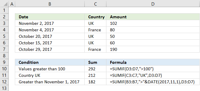
4. How to sum based on a condition applied to another column

The image above shows a formula in cell F3 that sums values from cell range C3:C7 if the corresponding value on the same row is equal to the condition specified in cell F3.
There are three cells that meet the condition, cells B3, B5, and B6. The corresponding values on the same rows in cell range C3:C7 are C3, C5, and C7.
The formula in cell F3 returns 212, 102 + 50 + 60 equals 212.
Formula in cell F3:
SUMIF function syntax:
SUMIF(range, criteria, [sum_range])
range - B3:B7
criteria - F2
[sum_range] - C3:C7
The sum_range is not the same as the range argument in this example, the sum_range argument is required.
5. How to sum if a number is smaller than a given condition

The picture above demonstrates a formula in cell E3 that adds numbers from cell range B3:B7 if they are below a condition specified in cell E2.
Cells B4, B5, and B6 meet the condition, 80 + 50 + 60 equals 190.
Note that cell E2 contains a "smaller than" character and a number, the SUMIF function works fine with logical operators.
Formula in cell E3:
SUMIF function syntax:
SUMIF(range, criteria, [sum_range])
range - B3:B7
criteria - E2
6. How to sum if a number is larger than a given condition

This example shows how to add numbers that are larger than a given condition and return a total.
The formula is in cell E3, it uses the condition specified in cell E2 to add numbers that meet the condition.
Numbers larger than 100 is added, they are 102 and 190 equals 292. The formula returns 292 in cell E3.
Formula in cell E3:
SUMIF function syntax:
SUMIF(range, criteria, [sum_range])
range - B3:B7
criteria - E2
7. How to sum based on a date

The image above demonstrates the SUMIF function using a date as a condition to add corresponding values and return a total.
The date is specified in cell F2, cells B4 and B6 match the date condition. 80 + 60 equals 140, the formula returns 140 in cell F3.
Excel dates are actually numbers formatted as Excel dates. 1/1/1900 is 1 and 1/1/2000 is 36526. You can verify this, type 1/1/1900 in cell, press Enter. Select the cell, press CTRL + 1 to open a dialog box "Format cells". Press with mouse on category "General", the number in the sample is now 1.
Formula in cell F3:
SUMIF function syntax:
SUMIF(range, criteria, [sum_range])
range - B3:B7
criteria - F2
[sum_range] - C3:C7
8. How to sum if a date is later than a given condition

This formula adds numbers from column C if the corresponding dates on the same row match the condition specified in cell F2.
Cells B5 and B7 match the condition in cell F2, the corresponding values in cells C5 and C7 are 50 and 190. 50 + 190 equals 240, formula in cell F3 returns 240.
Formula in cell F3:
SUMIF function syntax:
SUMIF(range, criteria, [sum_range])
range - B3:B7
criteria - F2
[sum_range] - C3:C7
9. How to sum if a date is earlier than a given condition

The image above demonstrates a formula in cell F3 that adds numbers from based on a condition in cell D2.
Cell B3 is the only cell that meets the condition in cell F2, dates must be earlier than or before the given date. Cell B3 contains 102 and the formula returns this number in cell F3.
Formula in cell F3:
SUMIF function syntax:
SUMIF(range, criteria, [sum_range])
range - B3:B7
criteria - F2
[sum_range] - C3:C7
10. How to use an asterisk to perform a wildcard match in the SUMIF function

The asterisk is a wild card character you can use to partially match a given string, the asterisk matches any number of characters.
Cell F2 contains an asterisk before and after the letter "w", this matches all cells that contain the letter "w".
Cells B5, B6, and B7 meet the given condition in cell F2, the corresponding cells are C5, C6, and C7. 10 + 30 + 20 equals 60, the formula in cell F3 returns 60.
Formula in cell F3:
SUMIF function syntax:
SUMIF(range, criteria, [sum_range])
range - B3:B7
criteria - F2
[sum_range] - C3:C7
11. How to use a question mark in the SUMIF function

The question mark ? is also a wildcard character, it matches any single character. Cell F2 contains "?AA" which matches cells B4, B7.
Why doesn't it match cell C8? Cell C8 begins with "C" which matches ?, however, the second character is "C" which does not match the second character in the condition which is "A".
Corresponding cells to B4 and B7 are C4 and C7. 20 + 20 equals 40, the formula in cell F3 returns 40.
Formula in cell F3:
SUMIF function syntax:
SUMIF(range, criteria, [sum_range])
range - B3:B8
criteria - F2
[sum_range] - C3:C8
12. How to sum numbers using a list of conditions

The SUMIF function can also sum numbers based on multiple conditions, however, make sure you enter it as an array formula because it returns as many sums as there are conditons.
The example above shows three conditions specified in cell range E3:E5.
Cells B6 and B8 match the condition in cell E3, the corresponding cells on the same rows are C6 and C8. They contain these numbers: 960 + 850 equals 1810.
Cells B4 and B11 match the condition in cell E5, the corresponding cells on the same rows are C4 and C11. They contain these numbers: 890 + 120 equals 1010.
Cells B3 and B5 match the condition in cell E5, the corresponding cells on the same rows are C3 and C5. They contain these numbers: 300 + 400 equals 700.
Array formula in cell range F3:F5:
SUMIF function syntax:
SUMIF(range, criteria, [sum_range])
range - B3:B11
criteria - E3:E5
[sum_range] - C3:C11
12.1 How to enter an array formula
Excel 365 users can ignore the following steps, enter the formula as a regular formula.
- Select cell range F3:F5.
- Type the formula in the formula bar.
- Press and hold CTRL + SHIFT simultaneously.
- Press Enter once.
- Release all keys.
The formula has a leading and trialing curly bracket, like this: {=SUMIF(B3:B11, E3:E5, C3:C11)}
They appear automatically, don't enter these characters yourself. See the image above, the formula bar has these characters.
13. How to sum not equal to

The picture above demonstrates a formula that adds numbers if the corresponding value on the same row is not equal to a given condition.
The condition uses a smaller than and a larger than characters combined to create a condition "not equal to". Cells B4 and B7 contain values that are not equal to the condition specified in cell F2.
The corresponding cells are C4 and C7 and they contain 80 + 190 equals 270. The formula in cell F3 returns 270.
Formula in cell F3:
SUMIF function syntax:
SUMIF(range, criteria, [sum_range])
range - H3:H7
criteria - M2
[sum_range] - J3:J7
14. How to sum by group
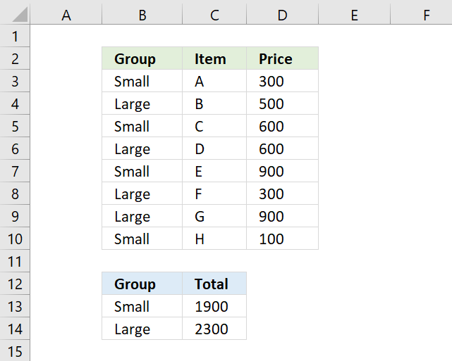
To extract groups from cell range B3:B10 I use the following regular formula in cell B13. The following formula is for Excel versions prior to Excel 365.
Copy cell B13 and paste to cell B14. Read this article to learn how this formula works.
To sum the numbers by group or value simply use this formula in cell C13.
Copy cell C13 and paste to cell C14.
14.1 Excel 365 formula
This formula in B13 is for Excel 365, it is called a dynamic array formula and is entered as a regular formula:
Enter this dynamic Excel 365 formula in cell B13.
14.2 Explaining formula
The SUMIF function sums cells that meet a condition, the first argument is the range you want to apply the criteria on. In this case cell range $B$3:$B$10, the $ (dollar signs) make the cell reference locked so when the formula is copied the reference stays the same.
The second argument is the criteria found in cell C13. That cell reference has no $ (dollar sign) so it changes when the formula is copied to the cell below. Why? We want it to use another group as a criterion in the next cell.
The third argument $D$3:$D$10 is the actual values we want to sum since they point to the same cell reference no matter where the formula is. It has a $ (dollar sign) that make it an absolute cell reference.
I highly recommend a pivot table if you have lots of data to work with.
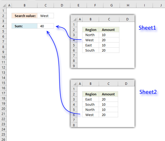
15. SUMIF across multiple sheets - Excel 365 formula

The image above shows three different worksheets: SUMIF, Sheet1, and Sheet2. The formula in cell C4 adds the amounts if the corresponding value on the same rows are equal to the specified condition in cell C2.
The example above has one match in Sheet1 on row 4 and one match in Sheet2 on row 6. They are 20 and 20 and the total is 40. The formula returns 40 in cell C4.
The SUMIF function is not going to accept an array (only cell range) in the first argument, we need to find a workaround. The SUM function works just as fine if we create a simple logical expression. See the below explanation for more details.
Excel 365 formula in cell C4:
SUM(
(INDEX(x,0,1)=C2)*INDEX(x,0,2)
)
)
15.1 Explaining formula
Step 1 - Stack arrays vertically
The VSTACK function combines cell ranges or arrays. Joins data to the first blank cell at the bottom of a cell range or array (vertical stacking)
Function syntax: VSTACK(array1,[array2],...)
VSTACK(Sheet1!B3:C6,Sheet2!B3:C6)
becomes
VSTACK(
{"North",10;
"West",20;
"East",10;
"South",20},
{"East",20;
"South",10;
"North",10;
"West",20})
and returns
{"North",10;
"West",20;
"East",10;
"South",20;
"East",20;
"South",10;
"North",10;
"West",20})
Step 2 - Get the first column from the stacked array
The INDEX function returns a value or reference from a cell range or array, you specify which value based on a row and column number.
Function syntax: INDEX(array, [row_num], [column_num])
INDEX(VSTACK(Sheet1!B3:C6,Sheet2!B3:C6),0,1)
becomes
INDEX({"North",10;
"West",20;
"East",10;
"South",20;
"East",20;
"South",10;
"North",10;
"West",20}),0,1)
and returns
{"North";
"West";
"East";
"South";
"East";
"South";
"North";
"West"})
Step 3 - Create logical expression
The equal sign is a logical operator, it lets you compare value to value. The result is a boolean value TRUE or FALSE. This also works with an array of values.
INDEX(VSTACK(Sheet1!B3:C6,Sheet2!B3:C6),0,1)=C2
becomes
{"North";
"West";
"East";
"South";
"East";
"South";
"North";
"West"})="West"
and returns
{FALSE; TRUE; FALSE; FALSE; FALSE; FALSE; FALSE; TRUE}
Step 4 - Get the second column from the stacked array
The INDEX function returns a value or reference from a cell range or array, you specify which value based on a row and column number.
Function syntax: INDEX(array, [row_num], [column_num])
INDEX(VSTACK(Sheet1!B3:C6,Sheet2!B3:C6),0,2)
becomes
INDEX(VSTACK({"North",10;
"West",20;
"East",10;
"South",20;
"East",20;
"South",10;
"North",10;
"West",20}),0,2)
and returns
{10;
20;
10;
20;
20;
10;
10;
20}
Step 5 - Multiply arrays
The asterisk lets you multiply numbers and boolean values in an Excel formula.
(INDEX(VSTACK(Sheet1!B3:C6,Sheet2!B3:C6),0,1)=C2)*INDEX(VSTACK(Sheet1!B3:C6,Sheet2!B3:C6),0,2)
becomes
{FALSE; TRUE; FALSE; FALSE; FALSE; FALSE; FALSE; TRUE} * {10; 20; 10; 20; 20; 10; 10; 20}
and returns
{0; 20; 0; 0; 0; 0; 0; 20}
Step 6 - Add numbers and return a total
The SUM function allows you to add numerical values, the function returns the sum in the cell it is entered in. The SUM function is cleverly designed to ignore text and boolean values, adding only numbers.
Function syntax: SUM(number1, [number2], ...)
SUM((INDEX(VSTACK(Sheet1!B3:C6,Sheet2!B3:C6),0,1)=C2)*INDEX(VSTACK(Sheet1!B3:C6,Sheet2!B3:C6),0,2))
becomes
SUM({0; 20; 0; 0; 0; 0; 0; 20})
and returns 40.
Step 7 - Shorten the formula
The LET function lets you name intermediate calculation results which can shorten formulas considerably and improve performance.
Function syntax: LET(name1, name_value1, calculation_or_name2, [name_value2, calculation_or_name3...])
SUM((INDEX(VSTACK(Sheet1!B3:C6,Sheet2!B3:C6),0,1)=C2)*INDEX(VSTACK(Sheet1!B3:C6,Sheet2!B3:C6),0,2))
x - VSTACK(Sheet1!B3:C6,Sheet2!B3:C6)
LET(x,VSTACK(Sheet1!B3:C6,Sheet2!B3:C6),
SUM(
(INDEX(x,0,1)=C2)*INDEX(x,0,2)
)
)
16. SUMIF across multiple sheets - User Defined Function
A User defined function is a custom function that anyone can build and use, you simply copy the code below and paste it to a code module in your workbook
This custom function works like the SUMIF function except that you can use multiple lookup and sum ranges.
Formula in cell C4:
16.1 User Defined Function Syntax
SUMIFAMS(lookup_value, lookup_range, sum_range)
16.2 Arguments
| Parameter | Text |
| lookup_value | Required. The value(s) you want to look for. |
| lookup_range | Required. The range you want to search. |
| sum_range | Required. The range you want to add. |
| [lookup_range_2] | Optional. You may have up to 127 additional argument pairs. |
| [sum_range_2] | Optional. |
16.3 VBA code
'Name function and arguments
Function SUMIFAMS(lookup_value As Range, ParamArray cellranges() As Variant)

'Declare variables and data types
Dim i As Integer, rng1 As Variant, temp As Single, a As Boolean
Dim rng2 As Variant, value As Variant, j As Single

'Make sure that the number of cell ranges are an even number. There must be a lookup_range and a sum_range.
If (UBound(cellranges) + 1) Mod 2 <> 0 Then

  'Display a message box.
  MsgBox "The number of range arguments must be even. 2, 4 , 8 ... and so on"

  'End function so the user can correct the problem.
  Exit Function
End If

'Iterate through all cell ranges
For i = LBound(cellranges) To UBound(cellranges) Step 2

    'Check that the number of rows in both cell ranges match
    If cellranges(i).Rows.Count <> cellranges(i + 1).Rows.Count Then
        MsgBox "The number of rows in range arguments don't match."
    End If

    'Make sure that the ranges only contain one column
    If cellranges(i).Columns.Count <> 1 Then
        MsgBox "Range arguments can only have size one column each."
        Exit Function
    End If

    'Save ranges to an array variable
    rng1 = cellranges(i).value
    rng2 = cellranges(i + 1).value

    'Iterate through values in array variable
    For j = LBound(rng1) To UBound(rng1)

        'Iterate through each lookup value if there is more than one
        For Each value In lookup_value

            'Make a comparison (not case sensitive)
            If UCase(rng1(j, 1)) = UCase(value) Then a = True
        Next value

        'Add the corresponding number to temp variable if a= True
        If a = True Then temp = temp + rng2(j, 1)
        a = False
    Next j
Next i
'Return total to worksheet
SumifAMS = temp
End Function
16.4 Where to copy vba code?
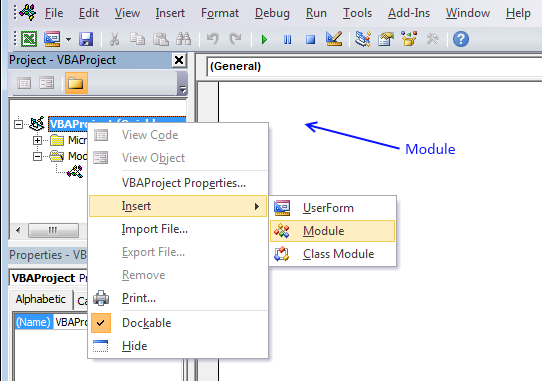
- Press Alt-F11 to open visual basic editor
- Press with left mouse button on Module on the Insert menu
- Copy and paste vba code.
- Exit visual basic editor
You can also use multiple search values, the returned number is a total based on both search values.

17. Function not working
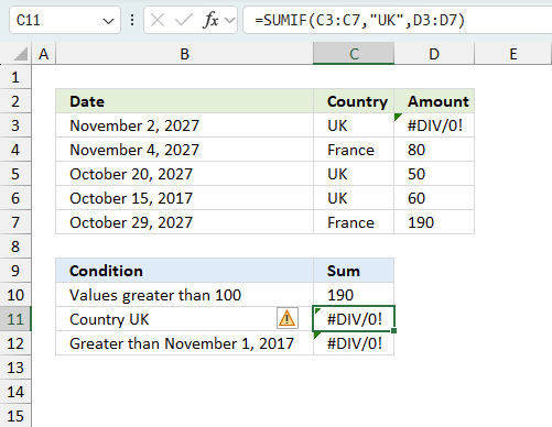
The SUMIF function returns a
- #NAME? error if you misspell the function name.
- propagates errors, meaning that if the input contains an error (e.g., #VALUE!, #REF!), the function will return the same error.
17.1 Troubleshooting the error value
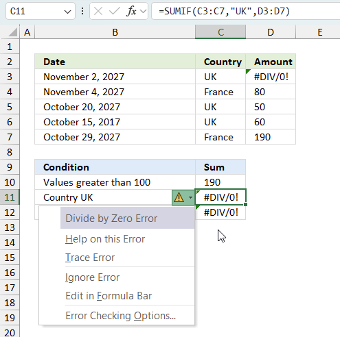
When you encounter an error value in a cell a warning symbol appears, displayed in the image above. Press with mouse on it to see a pop-up menu that lets you get more information about the error.
- The first line describes the error if you press with left mouse button on it.
- The second line opens a pane that explains the error in greater detail.
- The third line takes you to the "Evaluate Formula" tool, a dialog box appears allowing you to examine the formula in greater detail.
- This line lets you ignore the error value meaning the warning icon disappears, however, the error is still in the cell.
- The fifth line lets you edit the formula in the Formula bar.
- The sixth line opens the Excel settings so you can adjust the Error Checking Options.
Here are a few of the most common Excel errors you may encounter.
#NULL error - This error occurs most often if you by mistake use a space character in a formula where it shouldn't be. Excel interprets a space character as an intersection operator. If the ranges don't intersect an #NULL error is returned. The #NULL! error occurs when a formula attempts to calculate the intersection of two ranges that do not actually intersect. This can happen when the wrong range operator is used in the formula, or when the intersection operator (represented by a space character) is used between two ranges that do not overlap. To fix this error double check that the ranges referenced in the formula that use the intersection operator actually have cells in common.
#SPILL error - The #SPILL! error occurs only in version Excel 365 and is caused by a dynamic array being to large, meaning there are cells below and/or to the right that are not empty. This prevents the dynamic array formula expanding into new empty cells.
#DIV/0 error - This error happens if you try to divide a number by 0 (zero) or a value that equates to zero which is not possible mathematically.
#VALUE error - The #VALUE error occurs when a formula has a value that is of the wrong data type. Such as text where a number is expected or when dates are evaluated as text.
#REF error - The #REF error happens when a cell reference is invalid. This can happen if a cell is deleted that is referenced by a formula.
#NAME error - The #NAME error happens if you misspelled a function or a named range.
#NUM error - The #NUM error shows up when you try to use invalid numeric values in formulas, like square root of a negative number.
#N/A error - The #N/A error happens when a value is not available for a formula or found in a given cell range, for example in the VLOOKUP or MATCH functions.
#GETTING_DATA error - The #GETTING_DATA error shows while external sources are loading, this can indicate a delay in fetching the data or that the external source is unavailable right now.
17.2 The formula returns an unexpected value
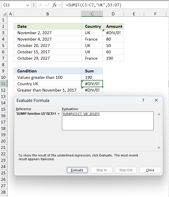
To understand why a formula returns an unexpected value we need to examine the calculations steps in detail. Luckily, Excel has a tool that is really handy in these situations. Here is how to troubleshoot a formula:
- Select the cell containing the formula you want to examine in detail.
- Go to tab “Formulas” on the ribbon.
- Press with left mouse button on "Evaluate Formula" button. A dialog box appears.
The formula appears in a white field inside the dialog box. Underlined expressions are calculations being processed in the next step. The italicized expression is the most recent result. The buttons at the bottom of the dialog box allows you to evaluate the formula in smaller calculations which you control. - Press with left mouse button on the "Evaluate" button located at the bottom of the dialog box to process the underlined expression.
- Repeat pressing the "Evaluate" button until you have seen all calculations step by step. This allows you to examine the formula in greater detail and hopefully find the culprit.
- Press "Close" button to dismiss the dialog box.
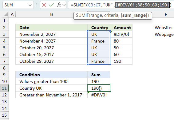
There is also another way to debug formulas using the function key F9. F9 is especially useful if you have a feeling that a specific part of the formula is the issue, this makes it faster than the "Evaluate Formula" tool since you don't need to go through all calculations to find the issue..
- Enter Edit mode: Double-press with left mouse button on the cell or press F2 to enter Edit mode for the formula.
- Select part of the formula: Highlight the specific part of the formula you want to evaluate. You can select and evaluate any part of the formula that could work as a standalone formula.
- Press F9: This will calculate and display the result of just that selected portion.
- Evaluate step-by-step: You can select and evaluate different parts of the formula to see intermediate results.
- Check for errors: This allows you to pinpoint which part of a complex formula may be causing an error.
The image above shows cell reference D3:D7 converted to hard-coded value using the F9 key. The SUMIF function requires non-error values which is not the case in this example. We have found what is wrong with the formula.
Tips!
- View actual values: Selecting a cell reference and pressing F9 will show the actual values in those cells.
- Exit safely: Press Esc to exit Edit mode without changing the formula. Don't press Enter, as that would replace the formula part with the calculated value.
- Full recalculation: Pressing F9 outside of Edit mode will recalculate all formulas in the workbook.
Remember to be careful not to accidentally overwrite parts of your formula when using F9. Always exit with Esc rather than Enter to preserve the original formula. However, if you make a mistake overwriting the formula it is not the end of the world. You can “undo” the action by pressing keyboard shortcut keys CTRL + z or pressing the “Undo” button
17.3 Other errors
Floating-point arithmetic may give inaccurate results in Excel - Article
Floating-point errors are usually very small, often beyond the 15th decimal place, and in most cases don't affect calculations significantly.
Get excel *.xlsx file
Useful links
'SUMIF' function examples
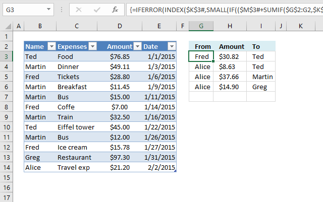
This article demonstrates two ways to calculate expenses evenly split across multiple people. The first one is a formula solution, […]
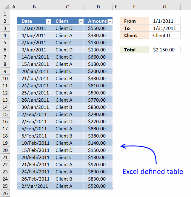
Excel 2010 has a PowerPivot feature and DAX formulas that let you work with multiple tables of data. You can […]
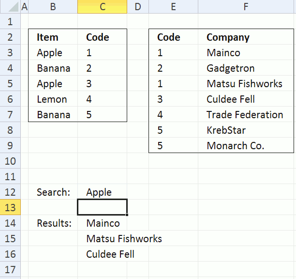
Andrew asks: LOVE this example, my issue/need is, I need to add the results. So instead of States and Names, […]
Functions in 'Math and trigonometry' category
The SUMIF function function is one of 62 functions in the 'Math and trigonometry' category.
Excel function categories
Excel categories
One Response to “How to use the SUMIF function”
Leave a Reply
How to comment
How to add a formula to your comment
<code>Insert your formula here.</code>
Convert less than and larger than signs
Use html character entities instead of less than and larger than signs.
< becomes < and > becomes >
How to add VBA code to your comment
[vb 1="vbnet" language=","]
Put your VBA code here.
[/vb]
How to add a picture to your comment:
Upload picture to postimage.org or imgur
Paste image link to your comment.
This was a very interesting technique. I've been trying to use something similar. Thanks for sharing.