Working with Relational Tables in Excel
Excel 2010 has a PowerPivot feature and DAX formulas that let you work with multiple tables of data. You can connect tables to each other based on relationships. When relationships are made nothing stops you from doing lookups to related values and relational tables or sum values for a relational table.
Table of Contents
- Introduction
- Search for values in a related table
- Search for values in a related table - Excel 365
- Sum values in a related table
- Sum values in a related table - Excel 365
- Get Excel *.xlsx file
- Search two related tables - VBA
- Search related table based on a date and date range
- Highlight lookups in relational tables
- Merge two relational data sets
- Working with three relational tables
- Extract unique distinct values from a relational table
1. Introduction
What is a relational table?
In a relational database (Microsoft Access), the data in one table is related to the data in other tables. In general, tables can be related in one of three different ways: one-to-one, one-to-many or many-to-many. The relationship is used to cross-reference information between tables.
Source: University of Sussex
This post is not about PowerPivot and DAX formulas, it is about doing lookups in two tables and they have one column in common. This means that the columns contain the same values, however, not necessarily in the same order. This makes the two data sets related because they share a value.
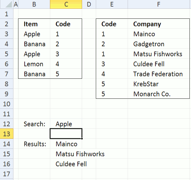
The image above shows a formula in cell C14 that looks for a value, specified in cell C12, in B3:B7. The corresponding value in C3:C7 is then used do a lookup in E3:E9. The formula then returns the corresponding values in F3:F9 to C14:C16. This is possible because they share the same values in column C and in column E.
Here is an example, cell C12 contains Apple, Apple is found in cell C3 and C5. The corresponding values in C3:C7 are 1 and 3. The formula looks for 1 and 3 in E3:E9 and finds cell E3, E5 and E6. Now the formula returns values from the same rows to C14:C16, the values are "Mainco", "Matsu Fishworks" and "Culdee Fell".
I'll also demonstrate a formula that sums values in a relational table.
2. Search for values in a related table

The animated image above explains how the concept works. The following formula can return a single value but it returns multiple values if more values match. Not only does it match multiple values in the first table, it also matches multiple values in the related table as well.
Array formula in cell C14:
How to create an array formula
- Select cell C14
- Copy above array formula
- Press with left mouse button on in formula bar
- Paste array formula
- Press and hold Ctrl + Shift
- Press Enter
How to copy array formula
- Select cell C14
- Copy (Ctrl + c)
- Select cell range C15:C17
- Paste (Ctrl + v)
Explaining array formula in cell C14
How can I examine formula calculations in greater detail?
You can follow formula calculations quite easily using the "Evaluate Formula" feature in Excel. Select cell C14 and then go to tab "Formulas" on the ribbon. Press with mouse on "Evaluate Formula" button to open an "Evaluate" dialog box.
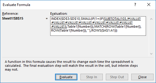
(The formula shown above in the Evaluate Formula" dialog box is not used in this article.)
Press with left mouse button on "Evaluate" button to see the next calculation step. I have demonstrated these calculations steps below.
Step 1 - Search for a value
The IF function has three arguments. IF(logical_test, [value_if_true], [value_if_false])
The logical_test argument contains an expression that either returns TRUE or FALSE, in this case the value in cell C12 is compared to all values in cell range B3:B7.
The corresponding value in cell range C3:C7 is returned if the expression returns TRUE and nothing is returned if FALSE.
IF($C$12=$B$3:$B$7, $C$3:$C$7, "")
becomes
IF("Apple"={"Apple"; "Banana"; "Apple"; "Lemon"; "Banana"}, {1; 2; 3; 4; 5}, "")
and returns {1;"";3;"";""}.
Step 2 - Use column in common to find matches
The MATCH function returns a number representing the relative position if a value exists in a cell range or array. It returns #N/A if not found.
MATCH($E$3:$E$9, IF($C$12=$B$3:$B$7, $C$3:$C$7, ""), 0)
becomes
MATCH($E$3:$E$9, {1;"";3;"";""}, 0)
becomes
MATCH({1; 2; 1; 3; 4; 5; 5}, {1;"";3;"";""}, 0)
and returns
{1;#N/A;1;3;#N/A;#N/A;#N/A}
Step 3 - Return row numbers
The ISERROR function is used to identify error values in the array, the IF function replaces error values with a blank "" and numbers with the corresponding row number.
IF(ISERROR(MATCH($E$3:$E$9, IF($C$12=$B$3:$B$7, $C$3:$C$7, ""), 0)), "", MATCH(ROW($F$3:$F$9), ROW($F$3:$F$9)))
becomes
IF(ISERROR({1;#N/A;1;3;#N/A;#N/A;#N/A}, "", MATCH(ROW($F$3:$F$9), ROW($F$3:$F$9)))
becomes
IF(ISERROR({1;#N/A;1;3;#N/A;#N/A;#N/A}, "", {1; 2; 3; 4; 5; 6; 7})
and returns {1; ""; 3; 4; ""; ""; ""}
Step 4 - Return a value of the cell at the intersection of a particular row and column
The corresponding row number is used by the INDEX function to return a specific value based on row and column numbers. The SMALL function extracts a row number based on a relative cell reference and the ROW function. The relative cell reference changes when the cell is copied and pasted to cells below.
=INDEX($F$3:$F$9, SMALL(IF(ISERROR(MATCH($E$3:$E$9, IF($C$12=$B$3:$B$7, $C$3:$C$7, ""), 0)), "", MATCH(ROW($F$3:$F$9), ROW($F$3:$F$9))), ROW(A1)))
becomes
=INDEX($F$3:$F$9, SMALL({1; ""; 3; 4; ""; ""; ""}, ROW(A1)))
becomes
=INDEX($F$3:$F$9, 1)
becomes
=INDEX({"Mainco"; "Gadgetron"; "Matsu Fishworks"; "Culdee Fell"; "Trade Federation"; "KrebStar"; "Monarch Co."}, 1)
and returns Mainco in cell C14.
3. Search for values in a related table - Excel 365

Excel 365 dynamic formula in cell F12:
Explaining the formula in cell F12
Step 1 - Compare values
The equal sign lets you compare value to value, in this case, value to values. The result is an array containing boolean values TRUE or FALSE.
B3:B7=C12
becomes
{"Apple"; "Banana"; "Apple"; "Lemon"; "Banana"}="Apple"
and returns
{TRUE; FALSE; TRUE; FALSE; FALSE}
Step 2 - Filter values based on a condition
The FILTER function extracts values/rows based on a condition or criteria.
Function syntax: FILTER(array, include, [if_empty])
FILTER(C3:C7,B3:B7=C12)
becomes
FILTER({1; 2; 3; 4; 5},{TRUE; FALSE; TRUE; FALSE; FALSE})
and returns
{1; 3}
Step 3 - Compare filtered values to values in the second table
The MATCH function returns the relative position of an item in an array that matches a specified value in a specific order.
Function syntax: MATCH(lookup_value, lookup_array, [match_type])
MATCH(E3:E9,FILTER(C3:C7,B3:B7=C12),0)
becomes
MATCH({1; 2; 1; 3; 4; 5; 5},{1; 3},0)
and returns
{1; #N/A; 1; 2; #N/A; #N/A; #N/A}
Step 4 - Check if an error has occurred
The IFNA function handles #N/A errors only, it returns a specific value if the formula returns a #N/A error.
Function syntax: IFNA(value, value_if_na)
IFNA(MATCH(E3:E9,FILTER(C3:C7,B3:B7=C12),0),0)
becomes
IFNA({1; #N/A; 1; 2; #N/A; #N/A; #N/A},0)
and returns
{1; 0; 1; 2; 0; 0; 0}
Step 5 - Filter values based on an array
It is possible to filter an array using numbers and not boolean values.
TRUE is the same as any number except 0 (zero).
FALSE is 0 (zero).
FILTER(F3:F9,IFNA(MATCH(E3:E9,FILTER(C3:C7,B3:B7=C12),0),0))
becomes
FILTER({"Mainco"; "Gadgetron"; "Matsu Fishworks"; "Culdee Fell"; "Trade Federation"; "KrebStar"; "Monarch Co."},{1; 0; 1; 2; 0; 0; 0})
and returns
{"Mainco"; "Matsu Fishworks"; "Culdee Fell"}
4. Sum values in a related table - earlier Excel versions

This example shows a formula that searches data in G3:G9 for a value specified in C12, uses the corresponding value on the same row in F3:F9 to match values in cell range C3:C7, and adds values on the same rows in cell range D3:D7 to calculate a total.
Formula in cell C14:
Explaining formula in cell C14

Step 1 - Find the relative position in the array
The MATCH function returns the relative position of an item in an array that matches a specified value in a specific order.
Function syntax: MATCH(lookup_value, lookup_array, [match_type])
MATCH(C12,G3:G9,0)
becomes
MATCH("Gadgetron",{"Culdee Fell"; "Gadgetron"; "KrebStar"; "Mainco"; "Matsu Fishworks"; "Monarch Co."; "Trade Federation"},0)
and returns 2.
Step 2 - Get value in cell range F3:F9
The INDEX function returns a value or reference from a cell range or array, you specify which value based on a row and column number.
Function syntax: INDEX(array, [row_num], [column_num])
INDEX(F3:F9,MATCH(C12,G3:G9,0))
becomes
INDEX(F3:F9,2)
and returns 2.
Step 3 - Get value in cell range F3:F9
The SUMIF function sums numerical values based on a condition.
Function syntax: SUMIF(range, criteria, [sum_range])
SUMIF(C3:C7,INDEX(F3:F9,MATCH(C12,G3:G9,0)),D3:D7)
becomes
SUMIF(C3:C7,2,D3:D7)
and returns 300.
5. Sum values in a related table - Excel 365

This example demonstrates an even smaller formula than the one in section 3. You need Excel 365 to use this formula.
Formula in cell C14:
Explaining the formula in cell C14
Step 1 - Compare values
The equal sign lets you compare values in an Excel formula, the result is either TRUE or FALSE.
C12=G3:G9
becomes
"Gadgetron"={"Culdee Fell"; "Gadgetron"; "KrebStar"; "Mainco"; "Matsu Fishworks"; "Monarch Co."; "Trade Federation"}
and returns
{FALSE; TRUE; FALSE; FALSE; FALSE; FALSE; FALSE}
Step 2 - Filter values
The Filter function extracts values/rows based on a condition or criteria.
Function syntax: FILTER(array, include, [if_empty])
FILTER(F3:F9,C12=G3:G9)
becomes
FILTER(F3:F9,{FALSE; TRUE; FALSE; FALSE; FALSE; FALSE; FALSE})
and returns 2.
Step 3 - Sum values
The SUMIF function sums numerical values based on a condition.
Function syntax: SUMIF(range, criteria, [sum_range])
SUMIF(C3:C7,FILTER(F3:F9,C12=G3:G9),D3:D7)
becomes
SUMIF({300;200;400;100;300},2,{1;2;3;2;5})
and returns 300.
7. Search two related tables - VBA
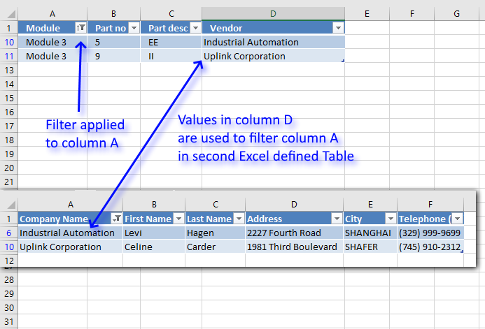
This section demonstrates a macro that automatically applies a filter to an Excel defined Table based on the result from a second Excel defined Table.
Let's say you do a lot of searches in two tables. The tables are related so it would be great if the second table is simultaneously filtered depending on the filtered values from the first table.
Two data sets are related if they share at least one column, that makes it possible to perform two searches or lookups.

Example,
You want to know the contact information to all vendors in product module 3. You select Module 3 in column "Product module" and vendor names appear in column "Vendor".
But contact information to each vendor is in table 2, sheet "Vendors". The macro demonstrated in the animated picture below filters table2 automatically.
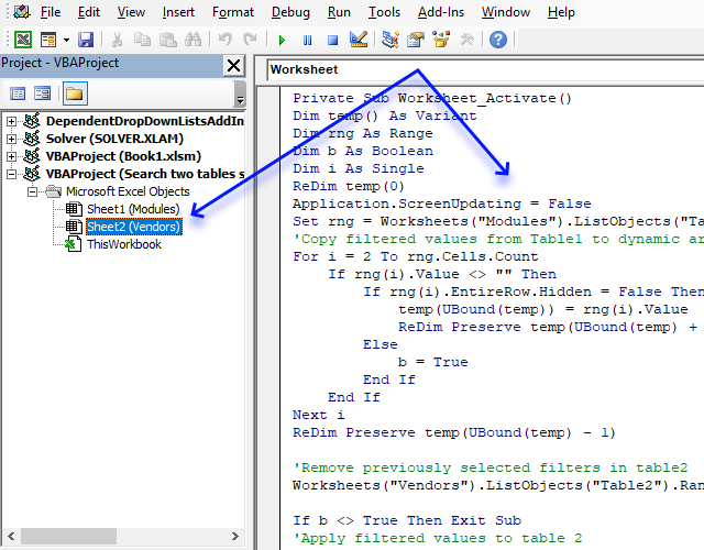
The following event code is rund when worksheet "Vendors" is activated.
'Event code that runs when worksheet is activated (selected)
Private Sub Worksheet_Activate()

'Dimension variables and declare data types
Dim temp() As Variant
Dim rng As Range
Dim b As Boolean
Dim i As Single

'Redimension variable temp to make it possible to add more values later on in this macro
ReDim temp(0)

'Don't show changes on screen
Application.ScreenUpdating = False

'Save the fourth column in Table1 to object variable rng
Set rng = Worksheets("Modules").ListObjects("Table1").ListColumns(4).Range

'Copy filtered values from Table1 to growing array

'Iterate through cells in cell range except header cell
For i = 2 To rng.Cells.Count

    'Check if value is not equal to nothing
    If rng(i).Value <> "" Then

        'Check that row is not filtered out
        If rng(i).EntireRow.Hidden = False Then

            'Save value to array variable temp
            temp(UBound(temp)) = rng(i).Value

            'Increase size of array variable temp
            ReDim Preserve temp(UBound(temp) + 1)
        Else

            'Save boolean value True to variable b, this will apply a filter to the other Excel defined Table later on in this event code
            b = True
        End If
    End If
Next i

'Remove last container from array variable temp
ReDim Preserve temp(UBound(temp) - 1)

'Remove previously selected filters in table2
Worksheets("Vendors").ListObjects("Table2").Range.AutoFilter Field:=1

'Check if variable b is False and stop this macro if so
If b <> True Then Exit Sub

'Apply filtered values to table 2
Worksheets("Vendors").ListObjects("Table2").Range.AutoFilter _
    Field:=1, Criteria1:=temp, Operator:=xlFilterValues

'Show changes to Excel user
Application.ScreenUpdating = True
End Sub
7.1 Where to put the code?
- Copy above event code.
- Press Alt + F11 to open the Visual Basic Editor.
- Doublepress with left mouse button on a worksheet in your workbook to open the worksheet module.
- Paste code to worksheet module.
8. Search related table based on a date and date range
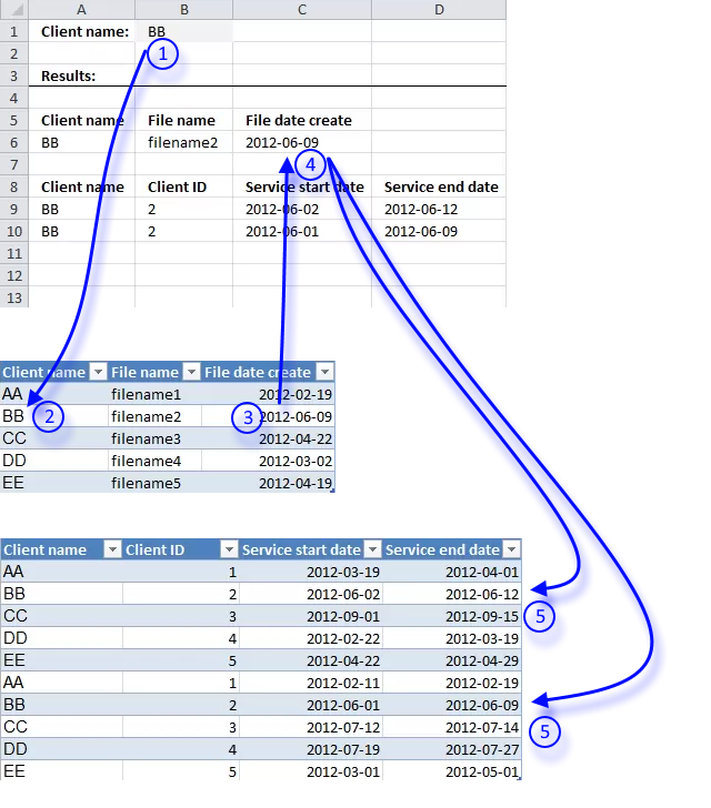
I will in this section demonstrate how to search a table for a date based on a condition and then use that date to search a second table based on the first lookup value and the returned date.
- The user enters a lookup value in cell B1.
- A formula finds the value in the first table.
- Then returns the corresponding date on the same rows as the found lookup value.
- The date is returned to cell C6.
- Another formula uses the returned date in cell C6 and the condition in cell B1 to search a second table . It then returns the matching records to cell range A9:D10 if the date is in the date range.
The formula in row 6 is really not necessary, it is only there so you can follow and understand the calculation.
Hi Oscar,I've been trying to find the solution for my lookup problem for a while now and you seem like the right person to ask... Your lookup code works great (thanks) but I need to do two or three lookups within identified matching records... in other words:
Sheet 1 - 'File data'
1. client name
2. filename
3. file date create
Sheet 2 - 'Client data'
1. client name
2. client ID
3. service start date
4. service end date
I need to map correct client ID based on lookup by client name and then based on finding which service date range does client file created date fit into.
So I need to:
1. First search - Identify Client records with matching name
2. Second search - Within that range, I need to find fitting date range.
Your lookups are great when I search entire sheets but I need to do second search based on subset of data.
Any help will be much appreciated.
Thanks!
Nena
Answer:
I created two tables containing random data.
Sheet1, Table1

Sheet2, Table2

Sheet 3:

Formula in cell A6:
This formula contains a reference to a table. Dragging the cell by the handle to 'pull' the formula across multiple columns won't work, it will mess up the structured references. You have to copy cell A6 and paste to cell range B6:C6.
Array formula in cell A9:
How to enter an array formula
- Select cell A9
- Press with left mouse button on in formula bar

- Paste above array formula
- Press and hold Ctrl + Shift
- Press Enter
Copy cell A9 and paste to cell range B9:D9. Copy cell range A9:D9 and paste to cell range A10:D14.
Explaining formula in cell A9
This formula does not need the calculations returned in row 6 in order to return the correct records.
Step 1 - Find the date
The MATCH function allows you to search a column for a specific value, it returns the relative position of the found value. For example, value "BB" is found in the second row so the MATCH function returns 2.
INDEX(Table1[File date create], MATCH(Sheet3!$B$1, Table1[Client name], 0))
becomes
INDEX(Table1[File date create], MATCH("BB", Table1[Client name], 0))
becomes
INDEX(Table1[File date create], MATCH("BB", {"AA"; "BB"; "CC"; "DD"; "EE"}, 0))
becomes
INDEX(Table1[File date create], 2)
and returns 6/9/2012. I recommend that you read How Excel Stores Times if you want to know how Excel handles dates.
Step 2 - Check if date is smaller than or equal to the end dates in Table2
The smaller than sign is a logical operator that compares the date to each date in column "Service end date" in Table 2, it returns TRUE or FALSE.
(INDEX(Table1[File date create], MATCH(Sheet3!$B$1, Table1[Client name], 0))<=Table2[Service end date])
becomes
(41069<={41000; 41072; 41167; 40987; 41028; 40958; 41069; 41104; 41117; 41030})
and returns {FALSE; TRUE; TRUE; FALSE; FALSE; FALSE; TRUE; TRUE; TRUE; FALSE}.
Step 3 - Check if date is larger than or equal to the start dates in Table2
The larger than sign is also a logical operator that compares the found date to each date in column "Service start date" in Table 2, it also returns TRUE or FALSE.
INDEX(Table1[File date create], MATCH(Sheet3!$B$1, Table1[Client name], 0))>=Table2[Service start date])
becomes
41069<=Table2[Service start date])
becomes
41069<={40987; 41062; 41153; 40961; 41021; 40950; 41061; 41102; 41109; 40969}
and returns
{FALSE; FALSE; TRUE; FALSE; FALSE; FALSE; FALSE; TRUE; TRUE; FALSE}
Step 4 - Check condition
The equal sign lets you compare the value in cell B1 to all values in column "Client name" in Excel Table named Table2.
$B$1=Table2[Client name]
becomes
"BB"={"AA"; "BB"; "CC"; "DD"; "EE"; "AA"; "BB"; "CC"; "DD"; "EE"}
and returns
{FALSE; TRUE; FALSE; FALSE; FALSE; FALSE; TRUE; FALSE; FALSE; FALSE}
Step 5 - Multiply arrays
All conditions must be TRUE in order to return the correct rows, we can accomplish that by multiplying all arrays.
The parentheses is used to control the order of calculation, we want to perform the comparisons before we multiply the arrays.
(INDEX(Table1[File date create], MATCH(Sheet3!$B$1, Table1[Client name], 0))<=Table2[Service end date])*(INDEX(Table1[File date create], MATCH(Sheet3!$B$1, Table1[Client name], 0))>=Table2[Service start date])*($B$1=Table2[Client name])
becomes
{FALSE; TRUE; TRUE; FALSE; FALSE; FALSE; TRUE; TRUE; TRUE; FALSE}*{FALSE; FALSE; TRUE; FALSE; FALSE; FALSE; FALSE; TRUE; TRUE; FALSE}*{FALSE; TRUE; FALSE; FALSE; FALSE; FALSE; TRUE; FALSE; FALSE; FALSE}
and returns
{0; 1; 0; 0; 0; 0; 1; 0; 0; 0}.
Step 6 - Return the corresponding row number
The IF function replaces the 1's with the corresponding row number and 0's with nothing (blank).
IF((INDEX(Table1[File date create], MATCH(Sheet3!$B$1, Table1[Client name], 0))<=Table2[Service end date])*(INDEX(Table1[File date create], MATCH(Sheet3!$B$1, Table1[Client name], 0))>=Table2[Service start date])*($B$1=Table2[Client name]), MATCH(ROW(Table2[Client name]), ROW(Table2[Client name])), "")
becomes
IF({0; 1; 0; 0; 0; 0; 1; 0; 0; 0}, MATCH(ROW(Table2[Client name]), ROW(Table2[Client name])), "")
becomes
IF({0; 1; 0; 0; 0; 0; 1; 0; 0; 0}, {1; 2; 3; 4; 5; 6; 7; 8; 9; 10}, "")
and returns
{"";2;"";"";"";"";7;"";"";""}.
Step 7 - Calculate k-th smallest row number
The SMALL function has the ability to return the k-th smallest number from a cell range or array.
SMALL(array, k)
SMALL(IF((INDEX(Table1[File date create], MATCH(Sheet3!$B$1, Table1[Client name], 0))<=Table2[Service end date])*(INDEX(Table1[File date create], MATCH(Sheet3!$B$1, Table1[Client name], 0))>=Table2[Service start date])*($B$1=Table2[Client name]), MATCH(ROW(Table2[Client name]), ROW(Table2[Client name])), ""), ROWS($A$1:A1))
becomes
SMALL({"";2;"";"";"";"";7;"";"";""}, ROWS($A$1:A1))
The ROWS function uses a cell reference that grows automatically when you copy the cell and paste to cells below, this allows the formula to return different values in each cell.
SMALL({"";2;"";"";"";"";7;"";"";""}, ROWS($A$1:A1))
becomes
SMALL({"";2;"";"";"";"";7;"";"";""}, 1)
and returns 2.
Step 8 - Return record
The INDEX function lets you fetch a value from a specific cell range based on a row number and a column number.
INDEX(Table2, SMALL(IF((INDEX(Table1[File date create], MATCH(Sheet3!$B$1, Table1[Client name], 0))<=Table2[Service end date])*(INDEX(Table1[File date create], MATCH(Sheet3!$B$1, Table1[Client name], 0))>=Table2[Service start date])*($B$1=Table2[Client name]), MATCH(ROW(Table2[Client name]), ROW(Table2[Client name])), ""), ROWS($A$1:A1)), COLUMNS($A$1:A1))
becomes
INDEX(Table2, 2, COLUMNS($A$1:A1))
The COLUMNS function uses a cell reference that grows automatically when you copy the cell and paste to cells to the right, this allows the formula to return different values in each cell.
INDEX(Table2, 2, COLUMNS($A$1:A1))
becomes
INDEX(Table2, 2, 1)
and returns "BB" in cell A9.
Step 9 - Remove errors
The IFERROR function removes errors when the formula runs out of values, however, be careful with this function. It removes all kinds of formula errors which may make it harder for you to troubleshoot and find errors.
9. Highlight lookups in relational tables
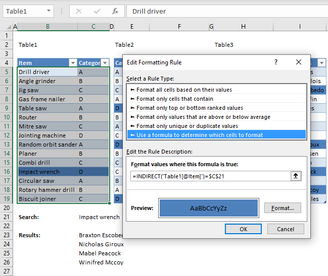
This article demonstrates a worksheet that highlights lookups across relational tables. I am using Excel defined Tables, if you add more rows to the Excel tables, the conditional formatting expands automatically.
The Excel user enters a value in cell C21 and the conditional formatting formulas applied to all three Excel Tables highlights values based on the relationship between tables and the search value.
The search value in cell C21 is found in B7, the corresponding value on the same row in Table1 is in cell C7. That value is used to do another lookup in column Category Table2 and four records are found.
Table2 has values in column Company in common with Table3 column Company, this relationship is used to highlight the corresponding values in column "Sales persons".
What is a relational table?
In a relational database (Microsoft Access), the data in one table is related to the data in other tables. In general, tables can be related in one of three different ways: one-to-one, one-to-many or many-to-many. The relationship is used to cross-reference information between tables.
Source: University of Sussex
How to apply Conditional Formatting?
- Select the first Excel Table (cell range B5:C19).
- Go to tab "Home" on the ribbon.
- Press with left mouse button on the "Conditional Formatting" button.
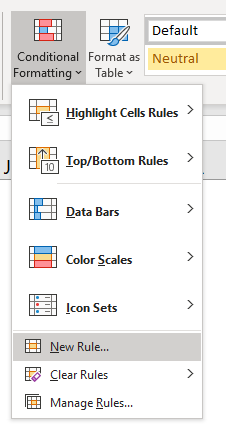
- Press with left mouse button on "New Rule..." and a dialog box appears.
- Press with left mouse button on "Use a formula to determine which cells to format".
- Type the formula below in "Format values where this formula is true:"
- Press with left mouse button on "Format" button.
- Go to tab "Fill.
- Pick a color.
- Press with left mouse button on OK button.
- Press with left mouse button on OK button.
- Repeat steps with the remaining Excel Tables and the corresponding CF formulas described below.
Conditional formatting formula applied to Excel Table Table1
You need to use the INDIRECT function to be able to reference an Excel defined Table in a Conditional Formatting formula. Table1[@Item] is a "structured reference" which is a way to reference Excel Tables, the @ character tells Excel to use only the cell in the same row as the Conditional Formatting formula in column Item.
This allows Excel to compare each value in column Item with the value specified in cell $C$21. This cell reference is an absolute cell reference which you can tell by the dollar characters ($). An absolute cell reference is locked to a specific cell and does not change when the Conditional Formatting formula moves to the next cell.
We do want it to always compare the value in cell C21 with all values in column Item, no matter what.
Conditional formatting formula applied to Excel Table Table2
Explaining Conditional Formatting formula in Table2
The steps below demonstrate what is calculated by the Conditional Formatting formula in cell E5.
Step 1 - Find matching items
The MATCH function returns the relative position of the matching value in column Item Table1.
MATCH($C$21, INDIRECT("Table1[Item]"), 0)
becomes
MATCH("Jig saw", {"Drill driver"; "Angle grinder"; "Jig saw"; "Gas frame nailer"; "Table saw"; "Router"; "Mitre saw"; "Jointing machine"; "Random orbit sander"; "Planer"; "Combi drill"; "Impact wrench"; "Circular saw"; "Rotary hammer drill"; "Biscuit joiner"}, 0)
and returns 3. "Jig saw" is on the third row in column Item Table1.
Step 2 - Return the value on the same row from column Category
The INDEX function returns a value from column Category based on the relative row number returned from the MATCH function.
INDEX(INDIRECT("Table1[Category]"), MATCH($C$21, INDIRECT("Table1[Item]"), 0))
becomes
INDEX(INDIRECT("Table1[Category]"), 3)
becomes
INDEX({"A";"B";"C";"D";"A";"B";"C";"D";"A";"B";"C";"D";"A";"B";"C"}, 3)
and returns "C".
Step 3 - Compare value in column Category Table 1 with Category Table2
INDEX(INDIRECT("Table1[Category]"), MATCH($C$21, INDIRECT("Table1[Item]"), 0))=INDIRECT("Table2[@Category]")
becomes
"C"=INDIRECT("Table2[@Category]")
becomes
"C"="A"
returns FALSE. Cell E5 in Table2 is not highlgihted.
Conditional formatting formula applied to Excel Table Table3

The animated image above shows what happens when different search conditions are used.
10. Merge two relational data sets
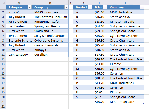
This section demonstrates how to merge two relational data sets before creating a Pivot table. A Pivot Table is limited to one table (data source) when you are working with relational data and I want to calculate the sales figures for each salesperson.
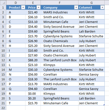
The image above shows one Excel table to the right that contains the product, price, and the company. The Excel Table to the left shows the salespersons and the corresponding company, a salesperson may work with multiple companies.
10.1. Create Excel Tables
I highly recommend Excel Tables, they save you a lot of time if you need to add more data to your data set and they have other useful features as well. You don't need to update the cell references each time you add data, however, you still need to refresh the Pivot Table.
- Select all cells you want to convert to an Excel Table.
- Press CTRL + T to create an Excel Table, a dialog box is displayed.
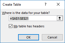
- Enable the checkbox if the Table has headers.
- Press with left mouse button on OK button.

Excel applies automatically cell formatting to a new Excel Table, you can change the Table style if you don't like it.
Select any cell in the Excel Table, go to tab "Table Design" on the ribbon and select a new Tables Style if you prefer something else.
10.2. Add a column to an Excel Table
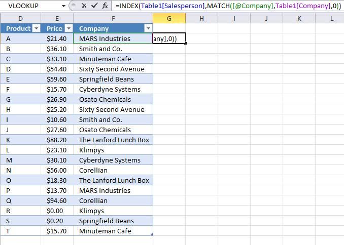
Excel expands the Excel defined Table automatically if you enter a value in an adjacent cell. Let's look for data in the first table [Table1].
- Select cell G2 which is the adjacent cell in this case, see image above.
- Type or copy/paste the following formula:
=INDEX(Table1[Salesperson], MATCH([@Company], Table1[Company], 0))
- Press Enter.
Another great feature is that the Excel defined Table automatically copies formulas to all cells in a column which you will see after you pressed Enter in the third step above.
10.2.1 Explaining formula
The formula you entered in cell G2 is actually better than a VLOOKUP formula, it allows you to search any column and the column you return values from is not hardcoded into the formula which may be a problem if you insert more columns to a data table.
Step 1 - Find relative position
The MATCH function has three arguments, the first argument is a cell reference to a cell on the same row in column Company as the cell you are currently adding the formula to. [@Company] It is called a structured reference and is special to Excel Tables.
[@Company] does not contain a reference to a Table name, the formula is located in the same Table so the Table name is not needed.
The second argument is a structured reference to all values in column Company in Table1 Table1[Company] and the third argument 0 (zero) tells Excel to perform an exact match.
MATCH(lookup_value, lookup_array, [match_type])
becomes
MATCH([@Company], Table1[Company], 0)
becomes
MATCH("MARS Industries", {"MARS Industries"; "The Lanford Lunch Box"; "Minuteman Cafe"; "Springfield Beans"; "Smith and Co."; "Sixty Second Avenue"; "Cyberdyne Systems"; "Osato Chemicals"; "Klimpys"; "Corellian"}, 0)
and returns 1. "MARS Industries" is in the first position in the array.
Step 2 - Get value
The INDEX function returns a value from a given cell range or array based on a row and column number. The column number is optional.
INDEX(array, [row_num], [column_num])
becomes
INDEX(Table1[Salesperson], MATCH([@Company], Table1[Company], 0))
becomes
INDEX(Table1[Salesperson], 1)
and returns the first value from column Salesperson in Table1 which is "Kirti Whitt".
The Excel Table has now the corresponding salesperson next to the company name.
If you are looking for more examples on merging two data lists, check this post: Merge lists with criteria
10.3. Create Pivot Table
If you are new to Pivot Tables don't freak out, they are so useful that I recommend you take time to get to know them better.
A Pivot Table allows you to quickly create totals based on conditions you specify, there is no need to build complicated formulas.
The speed the Pivot Table runs tasks is incredible. It is one of the greatest built-in features in Excel, in my opinion.
- Select any cell in Table2, the table to the right.
- Go to tab "Insert" on the ribbon.
- Press with left mouse button on "Pivot Table" button and a dialog box is diplayed, see image below.
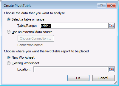
- Press with left mouse button on OK button. This will create an empty Pivot Table in a new worksheet.
10.4. Set up Pivot Table
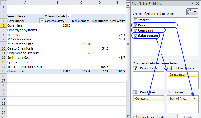
The image above shows a Pivot Table to the left and the corresponding task pane to the right. The task pane contains a list of fields based on headers in your Excel Table, you can drag these fields to different areas below which are:
- Report Filter
- Column Labels (horizontally)
- Row Labels (vertically)
- Values
Follow the simple instructions below see how much each salesperson has sold and to what company.
- Drag Price to Values area.
- Drag Company to Row Labels area.
- Drag Salesperson to Column Labels area.
The Report Filter lets you examine the data even deeper, simply drag a field to the Report Filter and a drop down list shows up above the Pivot Table. The drop down list contains items you may want to use as a filter condition.
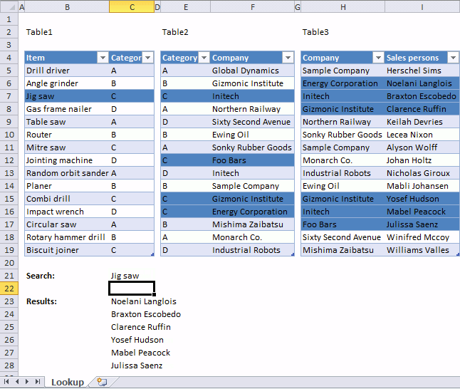
11. Working with three relational tables
I will in this section demonstrate four formulas that do lookups, extract unique distinct and duplicate values and sums numbers across three relational data sets using Excel formulas.
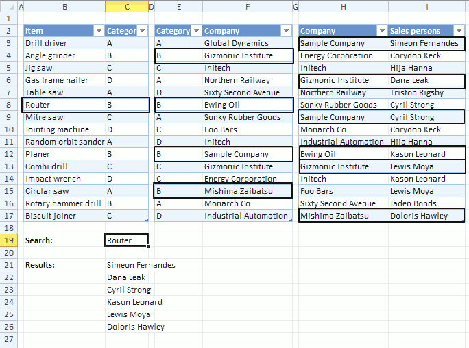
The image above shows a search value in cell C19, it is used as a search condition in column B and a matching value is found in cell B8. The corresponding value in column C is cell C8 which is then used do a second lookup in another table next to the first table.
The value in cell C8 is found in column E four times, they are E4, E8, E12 and E15. The formula now uses the values on the same row in column F to do a third lookup in column H.
Six matches are found in column H and the values on the same rows from colmn I are returned to cell range C21:C26.
What is a relational table?
In a relational database (Microsoft Access), the data in one table is related to the data in other tables. In general, tables can be related in one of three different ways: one-to-one, one-to-many or many-to-many. The relationship is used to cross-reference information between tables.
Source: University of Sussex
11.1 Lookups in three related tables and return multiple values

The animated picture above shows you how the array formula works, it looks for the Item "Router" in Item column in the first table (column B and C). The corresponding Category is B.
In table two (column E and F) there are 4 matches to Category "B". The corresponding companies in table 2 are "Gizmonic Institute", "Ewing Oil", "Sample Company" and "Mishima Zaibatsu".
In table 3 (column H and I) there are six matches to category "Company" and the adjacent Sales persons are returned in cell range C21:C27.
Array formula in cell range C21:
11.1.1 How to create an array formula
- Copy above array formula
- Select cell C21
- Press with left mouse button on in formula bar
- Paste array formula (Ctrl + v)
- Press and hold Ctrl+ Shift
- Press Enter
- Release all keys
The array formula is now surrounded by curly brackets, like this: {=array_formula}
11.1.2 How to copy array formula
- Select cell C21
- Copy cell (Ctrl + c)
- Select cell range C22:C27
- Paste (Ctrl + v)
11.1.3 Explaining lookup array formula in cell C21
Step 1 - Check whether a condition is met and return corresponding Table1[Category] value
IF($C$19=Table1[Item],Table1[Category],"")
becomes
IF("Router" = {"Drill driver"; "Angle grinder"; "Jig saw"; "Gas frame nailer"; "Table saw"; "Router"; "Mitre saw"; "Jointing machine"; "Random orbit sander"; "Planer"; "Combi drill"; "Impact wrench"; "Circlar saw"; "Rotary hammer drill"; "Biscuit joiner"}, {"A"; "B"; "C"; "D"; "A"; "B"; "C"; "D"; "A"; "B"; "C"; "D"; "A"; "B"; "C"} , "")
and returns
{"";"";"";"";"";"B";"";"";"";"";"";"";"";"";""}
Step 2 - Return the relative position of an item in an array that matches a specified value
MATCH(Table2[Category], IF($C$19=Table1[Item], Table1[Category], ""), 0)
becomes
MATCH(Table2[Category], {"";"";"";"";"";"B";"";"";"";"";"";"";"";"";""}, 0)
becomes
MATCH({"A"; "B"; "C"; "A"; "D"; "B"; "A"; "C"; "D"; "B"; "C"; "C"; "B"; "A"; "D"}, {"";"";"";"";"";"B";"";"";"";"";"";"";"";"";""}, 0)
and returns
{#N/A; 6; #N/A; #N/A; #N/A; 6; #N/A; #N/A; #N/A; 6; #N/A; #N/A; 6; #N/A; #N/A}
Step 3 - Check whether a condition is met and return corresponding Table2[Company] value
IF(ISERROR(MATCH(Table2[Category], IF($C$19=Table1[Item], Table1[Category], ""), 0)), "", Table2[Company])
becomes
IF(ISERROR({#N/A; 6; #N/A; #N/A; #N/A; 6; #N/A; #N/A; #N/A; 6; #N/A; #N/A; 6; #N/A; #N/A}), "", Table2[Company])
becomes
IF(ISERROR({#N/A; 6; #N/A; #N/A; #N/A; 6; #N/A; #N/A; #N/A; 6; #N/A; #N/A; 6; #N/A; #N/A}), "", {"Global Dynamics"; "Gizmonic Institute"; "Initech"; "Northern Railway"; "Sixty Second Avenue"; "Ewing Oil"; "Sonky Rubber Goods"; "Foo Bars"; "Initech"; "Sample Company"; "Gizmonic Institute"; "Energy Corporation"; "Mishima Zaibatsu"; "Monarch Co."; "Industrial Automation"})
and returns
{""; "Gizmonic Institute"; ""; ""; ""; "Ewing Oil"; ""; ""; ""; "Sample Company"; ""; ""; "Mishima Zaibatsu"; ""; ""}
Step 4 - Return the relative position of an item in an array that matches a specified value
MATCH(Table3[Company], IF(ISERROR(MATCH(Table2[Category], IF($C$19=Table1[Item], Table1[Category], ""), 0)), "", Table2[Company]), 0)
becomes
MATCH({"Sample Company"; "Energy Corporation"; "Initech"; "Gizmonic Institute"; "Northern Railway"; "Sonky Rubber Goods"; "Sample Company"; "Monarch Co."; "Industrial Automation"; "Ewing Oil"; "Gizmonic Institute"; "Initech"; "Foo Bars"; "Sixty Second Avenue"; "Mishima Zaibatsu"}, {""; "Gizmonic Institute"; ""; ""; ""; "Ewing Oil"; ""; ""; ""; "Sample Company"; ""; ""; "Mishima Zaibatsu"; ""; ""}, 0)
and returns
{10; #N/A; #N/A; 2; #N/A; #N/A; 10; #N/A; #N/A; 6; 2; #N/A; #N/A; #N/A; 13}
Step 5 - Check whether a condition is met and return row number
IF(ISERROR(MATCH(Table3[Company], IF(ISERROR(MATCH(Table2[Category], IF($C$19=Table1[Item], Table1[Category], ""), 0)), "", Table2[Company]), 0)), "", MATCH(ROW(Table3[Sales persons]), ROW(Table3[Sales persons])))
becomes
IF(ISERROR({10; #N/A; #N/A; 2; #N/A; #N/A; 10; #N/A; #N/A; 6; 2; #N/A; #N/A; #N/A; 13}), "", MATCH(ROW(Table3[Sales persons]), ROW(Table3[Sales persons])))
becomes
IF(ISERROR({10; #N/A; #N/A; 2; #N/A; #N/A; 10; #N/A; #N/A; 6; 2; #N/A; #N/A; #N/A; 13}), "", {1; 2; 3; 4; 5; 6; 7; 8; 9; 10; 11; 12; 13; 14; 15})
and returns
{1;"";"";4;"";"";7;"";"";10;11;"";"";"";15}
Step 6 - Return the k-th smallest row number
SMALL(array, k)
SMALL(IF(ISERROR(MATCH(Table3[Company], IF(ISERROR(MATCH(Table2[Category], IF($C$19=Table1[Item], Table1[Category], ""), 0)), "", Table2[Company]), 0)), "", MATCH(ROW(Table3[Sales persons]), ROW(Table3[Sales persons]))), ROW(A1))
becomes
SMALL({1;"";"";4;"";"";7;"";"";10;11;"";"";"";15}, ROW(A1))
and returns 1
Step 7 - Return a reference of the cell at the intersection of a particular row and column
INDEX(Table3[Sales persons], SMALL(IF(ISERROR(MATCH(Table3[Company], IF(ISERROR(MATCH(Table2[Category], IF($C$19=Table1[Item], Table1[Category], ""), 0)), "", Table2[Company]), 0)), "", MATCH(ROW(Table3[Sales persons]), ROW(Table3[Sales persons]))), ROW(A1)))
becomes
INDEX(Table3[Sales persons], 1)
becomes
INDEX({"Simeon Fernandes"; "Corydon Keck"; "Hija Hanna"; "Dana Leak"; "Triston Rigsby"; "Cyril Strong"; "Cyril Strong"; "Corydon Keck"; "Hija Hanna"; "Kason Leonard"; "Lewis Moya"; "Kason Leonard"; "Lewis Moya"; "Jaden Bonds"; "Doloris Hawley"}, 1)
and returns "Simeon Fernandes" in cell C21.
11.2 Filter unique distinct values from three related tables

There are two records of Salesperson "Simeon Fernandes" and Company "Sample Company" in the last table. Filtered Salespersons in cell range C21:C25 return Simeon Fernandes only once.
Array formula in cell range C21:
How to create an array formula
11.3 Filter duplicates from three related tables

Array formula in cell C21:
How to create an array formula
11.4 Sum values from three related tables

Array formula in cell C21:
How to create an array formula
12. Extract unique distinct values from a relational table
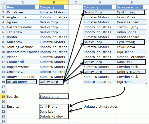
In this post, I am going to show you how to extract unique distinct values and duplicates using a formula, from a relational table. The image above shows a search value in cell B19, it is used by the formula to look for matches in A2:A16.
The formula finds a match in cell A16 and uses the corresponding value in cell B16 to do a second search in D2:D16, the two tables share values defined in B2:B16 and in D2:D16.
This makes it possible to perform searches across data sets, the value in cell B16 is found in cells D2, D8, D12 and D14. The corresponding cells in E2:E16 are E2, E8, E12 and E14, however, cell E2 and E8 contains duplicate values and the formula returns only one instance of those two values in cell range B21:B23.
In a previous post I described how to do lookups in a related table.
Table of Contents
- Unique distinct values
- Duplicate values
What is a relational table?
In a relational database (Microsoft Access), the data in one table is related to the data in other tables. In general, tables can be related in one of three different ways: one-to-one, one-to-many or many-to-many. The relationship is used to cross-reference information between tables. Source: University of Sussex
12.1 Unique distinct values

Array formula in cell B21:
To enter an array formula you copy above formula and paste to a cell. Press and hold CTRL and Shift simultaneously, then press Enter once. Release all keys.
The formula is now surrounded with curly brackets, don't enter these characters yourself, they appear automatically. {=formula}
Copy cell B21 and paste to cells below or simply select cell B21 and press and hold with left mouse button on the black dot located at the bottom right corner of the cell. Then drag with mouse down to cells below as far as needed, release left mouse button.
12.1.1 Explaining formula in cell B21
The "Evaluate formula" feature lets you examine a formula calculation in more detail, simply select cell B21 and then go to tab "Formulas" on the ribbon.
Press with mouse on "Evaluate formula" button to open the Evaluate Formula dialog box, the "Evaluate" button located on the dialog box takes you through the calculation step by step which is great if you want to troubleshoot or simply understand a formula.
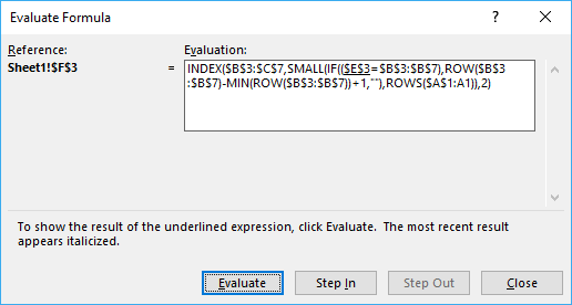
(The image above does not show the actual formula used in this example.)
Step 1 - Find values equal to search value
The IF function has three arguments, IF(logical_test, [value_if_true], [value_if_false]). The first argument contains a logical expression, it returns an array containing values TRUE or FALSE.
The second argument will run if the logical expression returns TRUE and the third will run if the value is FALSE.
IF($B$19=Table1[Item], Table1[Company], "")
becomes
IF("Biscuit joiner"=Table1[Item], Table1[Company], "")
becomes
IF("Biscuit joiner"={"Drill driver"; "Angle grinder"; "Jig saw"; "Gas frame nailer"; "Table saw"; "Router"; "Mitre saw"; "Jointing machine"; "Random orbit sander"; "Planer"; "Combi drill"; "Impact wrench"; "Circlar saw"; "Rotary hammer drill"; "Biscuit joiner"}, Table1[Company], "")
becomes
IF("Biscuit joiner"={"Drill driver"; "Angle grinder"; "Jig saw"; "Gas frame nailer"; "Table saw"; "Router"; "Mitre saw"; "Jointing machine"; "Random orbit sander"; "Planer"; "Combi drill"; "Impact wrench"; "Circlar saw"; "Rotary hammer drill"; "Biscuit joiner"}, {"Kumatsu Motors"; "Roboto Industries"; "Galaxy Corp"; "Galaxy Corp"; "Galaxy Corp"; "Roboto Industries"; "Kumatsu Motors"; "Roboto Industries"; "Roboto Industries"; "Kumatsu Motors"; "Kumatsu Motors"; "Kumatsu Motors"; "Roboto Industries"; "Kumatsu Motors"; "Galaxy Corp"}, "")
and returns
{"";"";"";"";"";"";"";"";"";"";"";"";"";"";"Galaxy Corp"}
Step 2 - Find relational values that corresponds to search value
The MATCH function returns the relative position of an item in an array or cell range that matches a specified value in a specific order.
MATCH(Table2[Company], IF($B$19=Table1[Item], Table1[Company], ""), 0)
becomes
MATCH(Table2[Company], {"";"";"";"";"";"";"";"";"";"";"";"";"";"";"Galaxy Corp"}, 0)
becomes
MATCH({"Galaxy Corp"; "Kumatsu Motors"; "Kumatsu Motors"; "Roboto Industries"; "Roboto Industries"; "Kumatsu Motors"; "Galaxy Corp"; "Kumatsu Motors"; "Roboto Industries"; "Roboto Industries"; "Galaxy Corp"; "Kumatsu Motors"; "Galaxy Corp"; "Kumatsu Motors"; "Roboto Industries"}, {"";"";"";"";"";"";"";"";"";"";"";"";"";"";"Galaxy Corp"}, 0)
and returns
{15; #N/A; #N/A; #N/A; #N/A; #N/A; 15; #N/A; #N/A; #N/A; 15; #N/A; 15; #N/A; #N/A}
This array shows us where the matches are in the column. 15 is in first, seventh, eleventh and thirteenth position.
Step 3 - Identify errors
The formula errors out if we don't get rid of the error values, the ISERROR function returns TRUE if the value is an error and FALSE if not.
ISERROR(MATCH(Table2[Company], IF($B$19=Table1[Item], Table1[Company], ""), 0))
becomes
ISERROR({15; #N/A; #N/A; #N/A; #N/A; #N/A; 15; #N/A; #N/A; #N/A; 15; #N/A; 15; #N/A; #N/A})
and returns
{FALSE; TRUE; TRUE; TRUE; TRUE; TRUE; FALSE; TRUE; TRUE; TRUE; FALSE; TRUE; FALSE; TRUE; TRUE}
step 4 - Avoid duplicate values
The COUNTIF function has two arguments COUNTIF(range, criteria), the first argument has an expanding cell reference that grows when the cell is copied to cells below. This makes it aware of previously displayed values and we can now avoid duplicates.
COUNTIF($B$20:B20,Table2[Sales persons])
becomes
COUNTIF("",Table2[Sales persons])
and returns
{0;0;0;0;0;0;0;0;0;0;0;0;0;0;0}
This array tells us that no values have been shown above cell B21.
Step 5 - Add arrays (OR logic)
By adding the two arrays we apply OR logic meaning that TRUE + TRUE = TRUE. FALSE + TRUE = TRUE. TRUE + FALSE = TRUE and FALSE + FALSE = FALSE.
Excel automatically converts boolean values to their numerical equivalents when the four basic arithmetic operations are preformed. Addition, subtraction, multiplication, and division.
(ISERROR(MATCH(Table2[Company], IF($B$19=Table1[Item], Table1[Company], ""), 0)))+COUNTIF($B$20:B20,Table2[Sales persons])
becomes
{FALSE; TRUE; TRUE; TRUE; TRUE; TRUE; FALSE; TRUE; TRUE; TRUE; FALSE; TRUE; FALSE; TRUE; TRUE} + {0;0;0;0;0;0;0;0;0;0;0;0;0;0;0}
and returns
{0;1;1;1;1;1;0;1;1;1;0;1;0;1;1}
Step 6 - Replace boolean values with row numbers and blanks
IF((ISERROR(MATCH(Table2[Company], IF($B$19=Table1[Item], Table1[Company], ""), 0)))+COUNTIF($B$20:B20,Table2[Sales persons]), "", MATCH(ROW(Table2[Company]), ROW(Table2[Company])))
becomes
IF({0;1;1;1;1;1;0;1;1;1;0;1;0;1;1}, "", MATCH(ROW(Table2[Company]), ROW(Table2[Company])))
becomes
IF({0;1;1;1;1;1;0;1;1;1;0;1;0;1;1}, "", {1; 2; 3; 4; 5; 6; 7; 8; 9; 10; 11; 12; 13; 14; 15})
and returns
{1;"";"";"";"";"";7;"";"";"";11;"";13;"";""}
Step 7 - Extract smallest row number
The SMALL function returns the smallest row number in the array.
SMALL(IF((ISERROR(MATCH(Table2[Company], IF($B$19=Table1[Item], Table1[Company], ""), 0)))+COUNTIF($B$20:B20,Table2[Sales persons]), "", MATCH(ROW(Table2[Company]), ROW(Table2[Company]))), 1)
becomes
SMALL({1;"";"";"";"";"";7;"";"";"";11;"";13;"";""}, 1)
and returns 1.
Step 8 - Return value from Table2[Sales persons]
The INDEx function returns a value from an array or cell range based on a row and column number.
INDEX(Table2[Sales persons], SMALL(IF((ISERROR(MATCH(Table2[Company], IF($B$19=Table1[Item], Table1[Company], ""), 0)))+COUNTIF($B$20:B20,Table2[Sales persons]), "", MATCH(ROW(Table2[Company]), ROW(Table2[Company]))), 1))
becomes
INDEX(Table2[Sales persons], 1)
becomes
INDEX({"Cyril Strong"; "Lewis Moya"; "Kason Leonard"; "Triston Rigsby"; "Jaden Bonds"; "Kason Leonard"; "Cyril Strong"; "Lewis Moya"; "Hija Hanna"; "Simeon Fernandes"; "Dana Leak"; "Corydon Keck"; "Doloris Hawley"; "Corydon Keck"; "Hija Hanna"}, 1)
and returns "Cyril Strong" in cell B21.
Step 9 - Remove error values
The IFERROR function removes errors that will show up when the formula runs out of values to display.
IFERROR(INDEX(Table2[Sales persons], SMALL(IF((ISERROR(MATCH(Table2[Company], IF($B$19=Table1[Item], Table1[Company], ""), 0)))+COUNTIF($B$20:B20,Table2[Sales persons]), "", MATCH(ROW(Table2[Company]), ROW(Table2[Company]))), 1)), "")
12.2 Duplicate values

Array formula in cell B21:
12.2.1 How to create an array formula
- Copy above array formula
- Select cell B21
- Press with left mouse button on in formula bar
- Paste (Ctrl + v)
- Press and hold Ctrl + Shift
- Press Enter
- Release all keys
The formula in the formula bar is now surrounded by curly brackets: {=array_formula}
12.2.2 How to copy an array formula
- Select cell B21
- Copy cell (Ctrl + c)
- Select cell range B22:B23
- Paste (Ctrl + v)
Related tables category
More than 1300 Excel formulasExcel categories
28 Responses to “Working with Relational Tables in Excel”
Leave a Reply
How to comment
How to add a formula to your comment
<code>Insert your formula here.</code>
Convert less than and larger than signs
Use html character entities instead of less than and larger than signs.
< becomes < and > becomes >
How to add VBA code to your comment
[vb 1="vbnet" language=","]
Put your VBA code here.
[/vb]
How to add a picture to your comment:
Upload picture to postimage.org or imgur
Paste image link to your comment.
[...] on Oct.17, 2012. Email This article to a Friend In a previous post I described how to do lookups in a related table. In this post I am going to show you how to extract unique distinct values and duplicates from a [...]
[...] values on Oct.19, 2012. Email This article to a Friend I have written a few posts about two related tables and today I am going to show you how to work with three related tables:Lookups in three related [...]
Its possible for me to get the regular updates from your site. Your site is excellent I ever seen.
Many Thanks
Chandra
[email protected]
Chandra,
thank you for your kind words!
You can subscribe to my blog updates by email or rss, see the right sidebar of this page.
[...] 0)), "", INDIRECT("Table2[Company]")), 0)))=FALSEYou can find the array formula in cell C23 here:Lookups in three related tables and return multiple values Get the Excel *.xlsx fileConditional formatting in related tables.xlsxRelated posts:Working with [...]
Oscar,
You are genius as your name.
Can you suggest me about site or vba book for vba excel as i did not found much about vba at your site get-digital-hel.
vijay singh
VIJAY SINGH,
I recommend "Excel 20xx Power Programming with VBA", author John Walkenbach.
Hi Oscar, your website has always come to my mind each time when I'm having difficulty with my Excel skill and I've learn alot from your post and thanks you very much for creating this for all of us to learn. I'm doing a reporting which need a similar function like what you has demostrate to us but I'll have 3 tab sheet for a product family name G1, G2 & G3 (which is manage by individual) plus a summary tab sheet.
Each of the product family tab sheet will have a shipment breakdown it consist of a schedule for shipment in the mode of Air, Ocean, Land. So how can I by choosing the date (which is the drop down list) it will show all the product in all the (G1, G2 & G3) which I intend to do it in the Summary tab sheet.
Once again, thanks for your help. Please let me know how can I upload my spreadsheet for your to understand more.
Best Regards,
Patrick
Patrick,
you can upload your workbook here: Upload
Or you could simply use PowerPivot or the Excel 2013 DataModel, and build a pivot from two linked tables.
Edouard,
I forgot to mention that!
Hi Oscar,
I failed to find right article in your blog and therefore I want to ask you in newest post. So I have table similar like this:
A 5
B 2
C 1
D 4
Is it possible with formula to generate list like this:
A
A
A
A
A
B
B
C
D
D
D
D
Thank you in advance!
BatTodor,
Read this post: Repeat values
[...] BatTodor asks: [...]
You are genius Oscar! :)
Thanks a lot!
Best regards
Todor
Hi,
I am looking for a inventory database. Can you help me in this. I am looking for excel tables to have sales data, purchase data and stock data date-wise.
Santosh,
You have email.
in excel sheet
i need to search three different word in eight sheet in particular cell and paste if present other wise blank
Example EE2203A,EE2204B,ME2201C
if present of any one paste EE2204B, other wise blank
karthikeyan,
can you explain in greater detail?
Hi Oscar,
You helped me out in the past, and I'm trying to understand the =Index(Match functions in an Array formula.
I have a range of data in 2 different columns on Sheet 2.
The ranges are almost identical, so much so that a simple "If" statement can show me differences.
. If they are equal display 1 else dispay 0. I don't want to filter as there is other data records in the sheet that are used in a vlookup formula.
So what would be the easiest way to have my first sheet "Sheet 1(A2)" find the "0" cells on Sheet 2 and display the values which are offset by 1 row?
In other words, for each two records on Sheet 2 that don't match, create a list of the 2nd record on "Sheet 1" with no blanks in between them.
Thanks in advance!
cwrbelis
cwrbelis,
Check the attached sheet:
cwrbelis.xlsx
Hi Oscar,
This is a question specific to your other article "How to extract a unique distinct list from a column in excel," but there wasn't a section to leave a reply, so I will ask it here.
I'm using your vba code for a user-defined function to extract unique distinct sorted values, but I want to use it in a table. As you probably know, multi-cell array formulas are not allowed in tables, so is there a way around this?
Thanks!
Hi Oscar,
I used your formula above, i have a question, it is possible to have a two search criteria?
Julius,
Yes it is.
Array formula in cell B21:
=IFERROR(INDEX(Table2[Sales persons], SMALL(IF((ISERROR(MATCH(Table2[Company], IF(COUNTIF($B$19:$C$19, Table1[Item]), Table1[Company], ""), 0)))+COUNTIF($B$20:B20,Table2[Sales persons]), "", MATCH(ROW(Table2[Company]), ROW(Table2[Company]))), 1)), "")
Hi Oscar,
I got two pivot tables from two sets of data ie Pivot table1 from data set1 and pivot table from data set2. I would like to know whether it is possible to control these pivot tables with a single slicer. The two data sets have common fields.
Hi Oscar,
I have two different tables, some row in both tables have same data, i want to extract unique rows data by comparing both tables... How can I do this...?
Hello Kamran Mumtaz
Great question, see this article:
https://www.get-digital-help.com/extract-unique-distinct-records-from-two-data-sets/
If I have a Matrix 2x10 in the following way
1 2 3 4 5 6 7 8 9 10
11 12 13 14 5 16 17 18 19 20
and want two arrange in the following way:
1 2
3 4
5 6
7 8
9 10
11 12
13 14
15 16
17 18
19 20
I have a large data file 8000x10 and the numbers are pair the first two number in first row will become first 2 numbers in first row , third and four in row 1 will be first and second in row 2, etc.