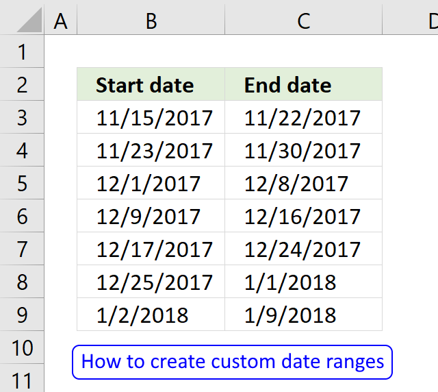
How to create date ranges in Excel
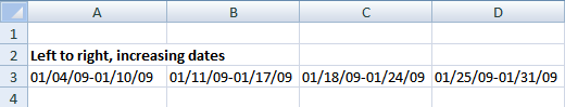
Cell A1 1/4/2009-1/10/2009
Cell B1 1/11/2009-1/17/2009
Cell C1 1/18/2009-1/24/2009
How do I create a formula to do this?
I will in this article discuss what Excel dates actually are, how to use them in formulas and how to create a sequence of dates that you can use as date ranges.
What is on this page?
- How to create date ranges in Excel
- Explaining Excel dates
- Basic date ranges
- Create a date sequence
- Advanced formula
- Explaining advanced formula
- Get workbook
- 7 days (weekly) date ranges using a formula
- Convert dates into date ranges
- Convert date ranges into dates - Excel 365
- Convert date ranges into dates - earlier Excel versions
- Create a quarterly date range using a clever built-in feature in Excel
- Quarterly date ranges using a formula
- Quarterly date ranges in one cell each
- Create a list of dates with blanks between quarters
- Create a monthly date range
1. How to create date ranges in Excel
1.1. What are dates in Excel?
First, what are dates in Excel? They are actually numbers and I will prove it to you, try these steps:
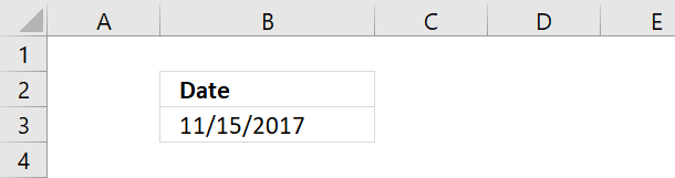
- Type a date in a cell
- Select the cell
- Press CTRL + 1 to open the "Format Cells" dialog box
- Select "General"
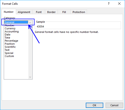
- Press with left mouse button on OK button
- The cell you selected now has a different formatting. This shows you what dates are in Excel.
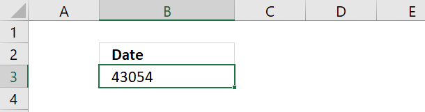
Date 11/15/2017 is 43054. Excel starts numbering dates at 1/1/1900 with value 1. Type 1 in a cell and change the cell formatting to "Date" and see what Excel displays.
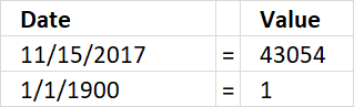
Date 11/15/2017 is 43053 days from 1/1/1900. This means also that you can't use dates prior to 1/1/1900.
Recommended articles
- How to format date values
- Calculate last date in month
- Find latest date based on a condition
- Workdays within date range
1.2. Basic date ranges
You can build a formula or use a built-in feature to build date ranges, read on to learn more.
Now you know that dates in Excel are numbers. You can easily create a date range by adding a number to a date.
The picture below shows a start date 11/15/2017, adding number 7 to that date returns 11/22/2017
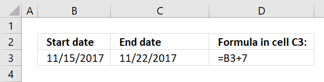
This allows you to quickly build date ranges simply by adding a number to a date.
Now select cell B4 and type =C3+1
Copy cell C3 and paste to cell C4.
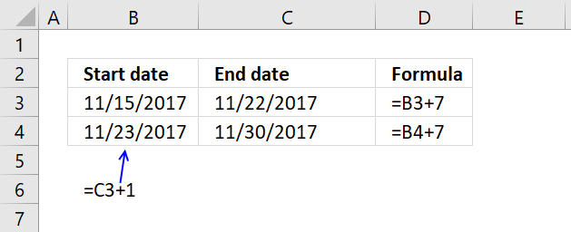
Relative cell references changes when you copy a cell and paste it to a new cell and I am going to use that now.
Copy cell range B4:C4 and paste it to cells below.
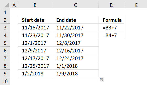
You have now built multiple date ranges using simple mathematics.
1.2.1 Create a date sequence
Excel has a great built-in feature that allows you to create number sequences in no time. Since dates are numbers in Excel you can use the same technique to build date ranges.
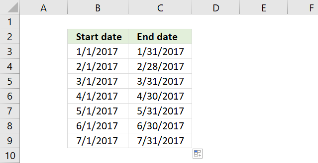
To build date ranges that have the same range but dates change, follow these steps:
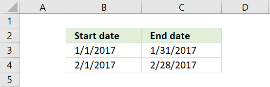
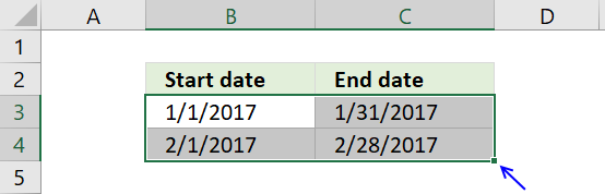
- Type the start date and the end date in a cell each
- Type the second start date an end date in cells below
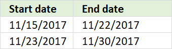
- Select both date ranges
- Press and hold on black dot
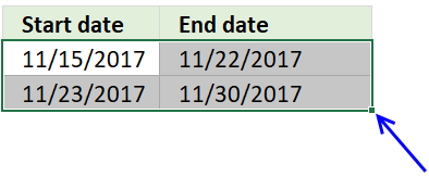
- Drag to cells below
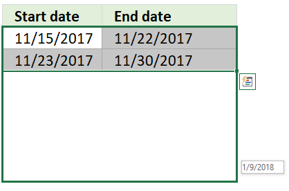
- Release mouse button
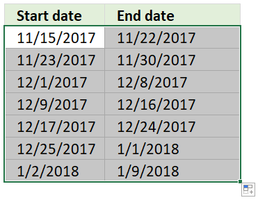
Excel has now built date ranges automatically using the two first date ranges as a template.
Recommended articles
- Use MEDIAN function to calculate overlapping ranges
- Identify overlapping date ranges
- Count overlapping days across multiple date ranges
- Find missing dates in a set of date ranges
1.3. Advanced formula

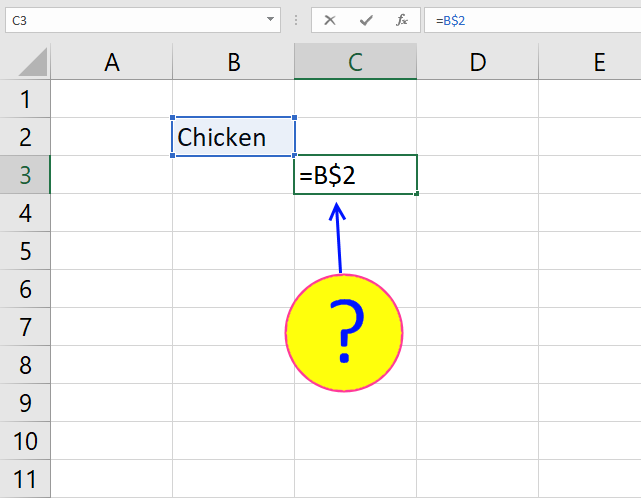
If you need to build date ranges that have both the start and end date in the same cell you need to build a more complicated formula. The TEXT function lets you format dates out of numbers.
See row 3 in the above picture.
1.3.1 Date ranges horizontally
The following formula returns date ranges that exists after the start date, the start date in this case is 1/4/2009, however you can easily change that.
The DATE function creates the number using three arguments. The first argument is the year, the second argument is the month and the third argument is the day.
DATE(year, month, day)
Formula in cell A3:
Copy cell A3 and paste to cells to the right as far as needed.
This formula returns date ranges that are prior to the given start date.
Formula in A6:
1.3.2 Date ranges vertically
Formula in A9:
Formula in A18:
1.3.3 How the formula in cell A3 works
The goal with the formula above is to create a date range from Sunday to Saturday. When cell A3 is copied and pasted to the right, the date range adjusts accordingly.
The formula consists of two parts. The first part calculates the start date of the date range. I have bolded the start date part of the formula below.
=TEXT(DATE(2009, 1, 4)+(COLUMNS($A:A)-1)*7, "mm/dd/yy")&"-"&TEXT(DATE(2009, 1, 4)+(COLUMNS($A:A)-1)*7+6, "mm/dd/yy")
Step 1 - First part of the formula creates the start date (bolded)
I have bolded the start date in this date range: 01/04/09 - 01/10/09.
TEXT(DATE(2009, 1, 4)+(COLUMNS($A:A)-1)*7, "mm/dd/yy")
DATE(2009, 1, 4) is the start date of the date range series.
DATE(2009, 1, 4) returns 39817
(COLUMN(A:A)-1)*7 creates a number determined by the current column.
COLUMNS($A:A) returns 1.
COLUMNS($A:A) - 1 returns 0.
(COLUMNS($A:A)-1)*7 returns 0.
This number creates how many days there is between start dates in the date ranges.
Start dates are bolded below.
Example
01/04/09 - 01/10/09 ; 01/11/09 - 01/17/09 ; 01/18/09 - 01/10/09
11 - 4 = 7, 18 - 11 = 7.
When the formula is copied and pasted to the right, the relative reference in COLUMNS($A:A) changes.
This cell reference changes as the formula is copied and pasted to the right.
Example,
COLUMNS($A:A) is 1
COLUMNS($A:B) is 2
COLUMNS($A:C) is 3
TEXT(DATE(2009, 1, 4)+0, "mm/dd/yy")
becomes
TEXT(39817 + 0, "mm/dd/yy").
"M/DD/YY" is the specified number format.
TEXT(39817 + 0, "mm/dd/yy") returns 01/04/09
Step 2 - Second part of the formula creates the end date
The second part of the formula is
TEXT(DATE(2009, 1, 4)+(COLUMNS($A:A)-1)*7+6, "mm/dd/yy")
The only difference between the first part of the formula:
TEXT(DATE(2009, 1, 4)+(COLUMNS($A:A)-1)*7, "mm/dd/yy")
and the second part of the formula:
TEXT(DATE(2009, 1, 4)+(COLUMNS($A:A)-1)*7+6, "mm/dd/yy")
is +6 (bolded)
Example
01/04/09 - 01/10/09
10 - 4 = 6
Recommended reading
Recommended articles
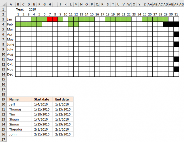
Table of Contents Plot date ranges in a calendar Plot date ranges in a calendar part 2 Highlight events in […]
2. 7 days (weekly) date ranges using a formula
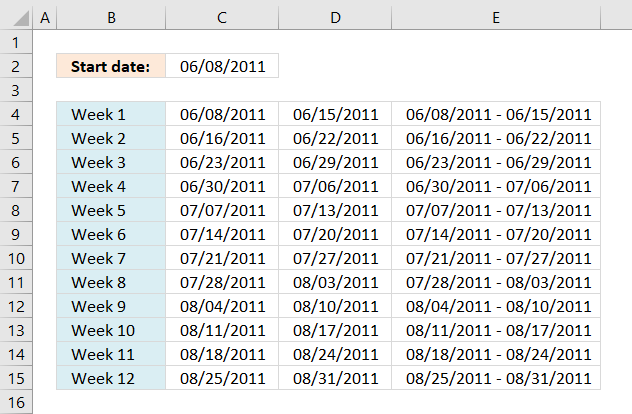
Shannon asks:I need a formula that if I enter a start date in field B1 such as 6/8/11 it will give me the date ranges for 7 days in fields B3-B14. Does that make sense?
Basically I want a formula that will tell me when a client is admitted to services on 6/8/11, their week 1 is 6/8/11 to 6/15/11; week 2 is 6/16/11-6/22/11 etc through 12 weeks.
I want the initial date in B1 to be the only value that I have to change to produce these results. Is that possible?
Answer:
I could create a big formula in cell range B3:B14 but instead, I am going to simplify formulas and use three columns.
The formulas are dynamic meaning when a date is entered in cell B1 cell range B3:D14 is instantly recalculated.
Formula in cell B3:
Formula in cell C3:
Copy (Ctrl + c) cell C3 and paste (Ctrl + v) to cell range C4:C14.
Formula in cell D3:
Copy (Ctrl + c) cell D3 and paste (Ctrl + v) to cell range D4:D14.
Formula in cell B4:
Copy (Ctrl + c) cell B4 and paste (Ctrl + v) to cell range B5:B14.
Explaining formula in cell C3
=$B$1+ROW(A1)*7
Step 1 - Create an absolute cell reference to start date
=$B$1+ROWS($A$1:A1)*7
$B$1 is an absolute cell reference. To create a reference to another cell, double press with left mouse button on cell C3. Type = and press with left mouse button on cell B1. The formula becomes =B1.
Let's convert the cell reference to an absolute cell reference. Absolute cell references are cell references that don't change when the cell is copied and pasted to another cell. Press F4.
The formula becomes: =$B$1.
Step 2 - Make dates with interval
=$B$1+ROW(A1)*7
ROW(A1). A1 is a relative cell reference to cell A1. A relative cell reference is a cell reference that adjusts and change when copied. ROW(A1) returns the row number of a reference. ROW(A1) returns 1.
ROW(A1)*7 becomes
1*7
and returns 7.
Step 3 - All together
=$B$1+ROW(A1)*7
becomes
40702+1*7
and returns 40709. Formatted as a date, cell C3 returns 6/15/11.
Cell C4 becomes =$B$1+ROW(A2)*7
=40702+2*7
becomes
=40702+14
and returns 40716. Formatted as a date, cell C4 returns 6/22/11.
9. Convert dates into date ranges

The array formula in cell D4 extracts the start dates for date ranges in cell range B3:B30, the array formula in cell E4 extracts the end dates for date ranges in cell range B3:B30.
The dates in column B must be sorted from smallest to largest for the formula to work properly, the image above shows the date ranges (blue lines) and the numbers correspond to the extracted date ranges displayed in column D and E.
Excel 365 formula in cell D4:
The cells above (B2) and below (B31) cell range B3:B30 must be empty for the Excel 365 formula to work properly.
Array formula in cell D4:
How to create an array formula
- Select cell C2
- Paste formula
- Press and hold CTRL + SHIFT
- Press Enter
Copy cell C2 and paste it down as far as needed.
Array formula in cell E4:
Copy cell D2 and paste it down as far as needed.
Explaining formula in cell D5
The formula extracts the first date if the current cell is the first cell that is why I start with formula in cell D5.
The ROWS function returns the number of rows in a cell reference, when the cell is copied to cells below the cell reference grows, this is how the formula keeps track of where the first cell is.
IF(ROWS($B$2:B2)=1,INDEX($B$3:$B$30,1), formula)
ROWS($B$2:B2)=1
becomes
1=1 equals TRUE.
IF(TRUE,INDEX($B$3:$B$30,1), formula)
becomes
INDEX($B$3:$B$30,1)
and returns the first date in cell $B$3:$B$30 (1/1/2010).
Step 1 - Compare dates
If we subtract a date with the next date in a sorted list we can quickly check if the next date is one day after the first date. If the number is larger than 1 we know the first date must be an end date and the next date must be a start date.
$B$4:$B$30-$B$3:$B$29>1
returns {FALSE; FALSE; TRUE; ... ; FALSE}
Step 2 - Replace TRUE with corresponding row number
The IF function has three arguments, the first one must be a logical expression. If the expression evaluates to TRUE then one thing happens (argument 2) and if FALSE another thing happens (argument 3).
IF($B$4:$B$30-$B$3:$B$29>1,ROW($B$3:$B$29)-MIN(ROW($B$3:$B$29))+2,"")
returns {""; ""; 4; ... ; ""}.
Step 3 - Extract k-th smallest row number
The SMALL function lets you calculate the k-th smallest value in a cell range or array. SMALL( array, k). This makes sure that a new date is displayed in each cell below. The k argument contains an expanding cell reference that grows when the cell is copied to cells below.
SMALL(IF($B$4:$B$30-$B$3:$B$29>1, ROW($B$3:$B$29)-MIN(ROW($B$3:$B$29))+2, ""), ROWS($B$1:B2)-1)
returns 4.
Step 4 - Return value
The INDEX function returns a value based on a cell reference and column/row numbers.
INDEX($B$3:$B$30,SMALL(IF($B$4:$B$30-$B$3:$B$29>1,ROW($B$3:$B$29)-MIN(ROW($B$3:$B$29))+2,""),ROWS($B$1:B1)-1))
returns 1/5/2010 in cell D5.
10. Convert date ranges into dates - Excel 365

This section shows an Excel 365 formula that lists dates based on multiple date ranges, it spills values automatically to cells below.
Excel 365 formula in cell B3:
Explaining formula
Step 1 - Calculate days in each date range
The minus sign lets you subtract numbers in an Excel formula.
E4:E8-D4:D8
becomes

and returns
{2;4;0;16;1}.
Step 2 - Create a sequence of numbers from 0 to n
The SEQUENCE function creates a list of sequential numbers.
Function syntax: SEQUENCE(rows, [columns], [start], [step])
SEQUENCE(,x+1,0)
x is a variable in the LAMBDA function that represents each value in the array: {2;4;0;16;1}
The SEQUENCE function creates a new sequence for each number in the array.
Step 3 - Stack arrays vertically
The VSTACK function combines cell ranges or arrays. Joins data to the first blank cell at the bottom of a cell range or array (vertical stacking)
Function syntax: VSTACK(array1,[array2],...)
VSTACK(acc,SEQUENCE(,x+1,0))
The VSTACK function adds each sequence to an accumulator variable named acc.
Step 4 - Build LAMBDA function
The LAMBDA function build custom functions without VBA, macros or javascript.
Function syntax: LAMBDA([parameter1, parameter2, …,] calculation)
LAMBDA(acc,x,VSTACK(acc,SEQUENCE(,x+1,0)))
The LAMBDA function lets you name parameters you need in order to properly use the REDUCE function.
Step 5 - Build REDUCE function
The REDUCE function shrinks an array to an accumulated value, a LAMBDA function is needed to properly accumulate each value in order to return a total.
Function syntax: REDUCE([initial_value], array, lambda(accumulator, value))
REDUCE(0,E4:E8-D4:D8,LAMBDA(acc,x,VSTACK(acc,SEQUENCE(,x+1,0))))
returns

Excel fills empty array contains with error values. We need to take care of this in the last step.
Step 6 - Remove first row in array
The DROP function removes a given number of rows or columns from a 2D cell range or array.
Function syntax: DROP(array, rows, [columns])
DROP(REDUCE(0,E4:E8-D4:D8,LAMBDA(acc,x,VSTACK(acc,SEQUENCE(,x+1,0)))),1)
returns the following array:

The first row in the array is deleted. Why is this row in there? It is the first argument 0 in the REDUCE function that creates the first row in the array.
Step 7 - Add start dates to number sequences
The plus sign lets you add numbers in an Excel formula. Excel dates are actually numbers so this method allows us to create date sequences.
D4:D8+DROP(REDUCE(0,E4:E8-D4:D8,LAMBDA(acc,x,VSTACK(acc,SEQUENCE(,x+1,0)))),1)
becomes

and returns

Step 8 - Rearrange array to one column
The TOCOL function rearranges values in 2D cell ranges to a single column.
Function syntax: TOCOL(array, [ignore], [scan_by_col])
TOCOL(D4:D8+DROP(REDUCE(0,E4:E8-D4:D8,LAMBDA(acc,x,VSTACK(acc,SEQUENCE(,x+1,0)))),1))
returns

Step 9 - Extract unique dates
The UNIQUE function returns a unique or unique distinct list.
Function syntax: UNIQUE(array,[by_col],[exactly_once])
UNIQUE(TOCOL(D4:D8+DROP(REDUCE(0,E4:E8-D4:D8,LAMBDA(acc,x,VSTACK(acc,SEQUENCE(,x+1,0)))),1)))
returns

The fourth value is an error value. This value will be last when we sort the array in the next step.
Step 10 - Sort dates from small to large
The SORT function sorts values from a cell range or array
Function syntax: SORT(array,[sort_index],[sort_order],[by_col])
SORT(UNIQUE(TOCOL(D4:D8+DROP(REDUCE(0,E4:E8-D4:D8,LAMBDA(acc,x,VSTACK(acc,SEQUENCE(,x+1,0)))),1))))
returns

Step 11 - Remove last row in array
The DROP function removes a given number of rows or columns from a 2D cell range or array.
Function syntax: DROP(array, rows, [columns])
DROP(SORT(UNIQUE(TOCOL(D4:D8+DROP(REDUCE(0,E4:E8-D4:D8,LAMBDA(acc,x,VSTACK(acc,SEQUENCE(,x+1,0)))),1)))),-1)
The last value in the array is an error value, the DROP function removes the last value from the array.
11. Convert date ranges into dates - earlier Excel versions
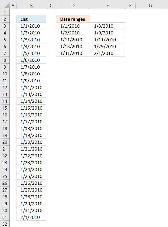
The array formula in cell B3 creates a list of dates based on the date ranges displayed in D3:E7, it handles overlapping date ranges, however, only one instance of each overlapping date is shown.
Array formula in cell B3:
How to create an array formula
- Copy above array formula
- Select cell B3
- Press with left mouse button on in formula bar

- Paste array formula in formula bar
- Press and hold Ctrl + Shift
- Press Enter
- Release all keys
How to copy array formula
- Select cell B3
- Copy cell (Ctrl + c)
- Select cell range B3:B30
- Paste (Ctrl + v)
Explaining formula in cell B3
Step 1 - Create a dynamiccell reference
This step calculates the first date and the last date of all date ranges and builds a cell reference with as many rows as there are days between the first date and the last date.
The MIN function returns the smallest number (date) from all date ranges and the MAX function returns largest number (date) from all date ranges.
$B$1:INDEX($B:$B, MAX($D$3:$E$7)-MIN($D$3:$E$7)+1)
becomes
$B$1:INDEX($B:$B, 40210-40179+1)
becomes
$B$1:INDEX($B:$B, 32)
and returns
$B$1:$B$32
Step 2 - Create a sequence of values
The ROW function creates a sequence of numbers between 0 (zero) and n based on the number of rows in the cell reference.
ROW($B$1:INDEX($B:$B, MAX($D$3:$E$7)-MIN($D$3:$E$7)+1))-1
becomes
ROW($B$1:$B$32)-1
and returns
{0; 1; 2; ... ; 31}.
Step 3 - Create an array of dates
"<="&MIN($D$3:$E$7)+ROW($B$1:INDEX($B:$B, MAX($D$3:$E$7)-MIN($D$3:$E$7)+1))-1
returns {"<=40179"; "<=40180"; ... ; "<=40210"}
The less than sign and equal sign is there to check if dates are inside the date range, this is calculated in the next step.
Step 4 - Calculate if date is in date range
The COUNTIFS function calculates the number of cells across multiple ranges that equals all given conditions.
COUNTIFS($D$3:$D$7, "<="&MIN($D$3:$E$7)+ROW($B$1:INDEX($B:$B, MAX($D$3:$E$7)-MIN($D$3:$E$7)+1))-1, $E$3:$E$7, ">="&MIN($D$3:$E$7)+ROW($B$1:INDEX($B:$B, MAX($D$3:$E$7)-MIN($D$3:$E$7)+1))-1)
returns
{1; 2; 2; 1; 1; 1; 1; 1; 1; 0; 1; 0; 1; 1; 1; 1; 1; 1; 1; 1; 1; 1; 1; 1; 1; 1; 1; 1; 1; 0; 1; 1}
A 0 (zero) indicates that the date is not in a date range, 1 means that the date is in one date range, 2 means two dates ranges and so on.
Step 5 - Replace any number except 0 (zero) with corresponding date
The IF function has three arguments, the first one must be a logical expression. If the expression evaluates to TRUE then one thing happens (argument 2) and if FALSE another thing happens (argument 3).
IF(COUNTIFS($D$3:$D$7, "<="&MIN($D$3:$E$7)+ROW($B$1:INDEX($B:$B, MAX($D$3:$E$7)-MIN($D$3:$E$7)+1))-1, $E$3:$E$7, ">="&MIN($D$3:$E$7)+ROW($B$1:INDEX($B:$B, MAX($D$3:$E$7)-MIN($D$3:$E$7)+1))-1), MIN($D$3:$E$7)+ROW($B$1:INDEX($B:$B, MAX($D$3:$E$7)-MIN($D$3:$E$7)+1))-1, "")
returns {40179; 40180; ... ; 40210}.
Step 6 - Extract k-th smallest date
To be able to return a new value in a cell each I use the SMALL function to filter date numbers from smallest to largest.
SMALL(IF(COUNTIFS($D$3:$D$7, "<="&MIN($D$3:$E$7)+ROW($B$1:INDEX($B:$B, MAX($D$3:$E$7)-MIN($D$3:$E$7)+1))-1, $E$3:$E$7, ">="&MIN($D$3:$E$7)+ROW($B$1:INDEX($B:$B, MAX($D$3:$E$7)-MIN($D$3:$E$7)+1))-1), MIN($D$3:$E$7)+ROW($B$1:INDEX($B:$B, MAX($D$3:$E$7)-MIN($D$3:$E$7)+1))-1, ""), ROWS($B$1:B1))
eturns 1/1/2010 in cell B3.
Useful links
Format an Excel date the way you want
How to change date format in Excel and create custom formatting
12. Create a quarterly date range using a clever built-in feature in Excel

Excel lets you copy formulas and data using the fill handler, a handy tool that automates your work. It is also smart enough to create number sequences.
Conveniently Excel dates are in fact numbers so the fill handler works fine with dates, as well.
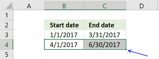
Type the start and end date of the first quarterly date range in row 3. Type the second date range in row 4, see picture below.
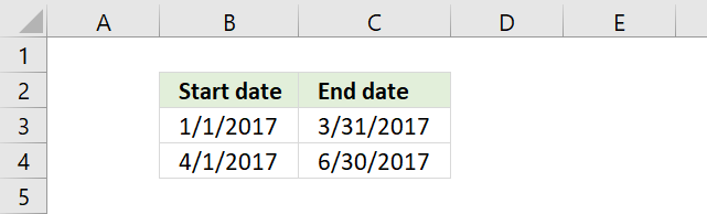
Select cell range B3:C4. Press and hold on the black dot.
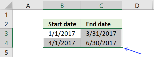
Drag to cells below as far as needed.
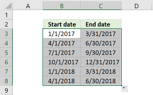
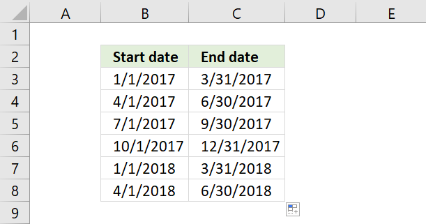
Excel automatically creates the following date ranges using the selected cells as a guide to determine the range and starting point.
13. Quarterly date ranges using a formula
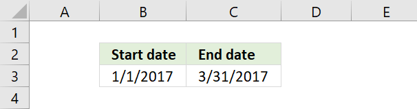
You also have the option to build a date range using formulas. I have entered 1/1/2017 in cell B3 and the following formula in cell C3:
See picture below. The formula adds 3 months to the date in cell B3 and then subtracts 1 to get the last date for the first quarterly date range. This setup takes into account that months have 30 or 31 days.
Type this formula in cell B4:
It is almost identical to the formula in cell C3. Then copy cell C3 and paste to cell C4.
Now select cell range B4:C4 and press and hold on black dot, see picture above.
Drag to cells below as far as needed. This action copies the formulas in cell range B4:C4 and pastes them to cells below.
14. Date ranges in one cell each
The following picture shows date ranges in a cell each, to achieve that we need to build a somewhat more complicated formula. The formulas in cell A4 and A7 must be copied to cells to the right of the start cell.

Array formula in A4:
copied right as far as necessary.
Array formula in A7:
copied right as far as necessary.
Array formula in A10:
copied down as far as necessary.
Array formula in A17:
copied down as far as necessary.
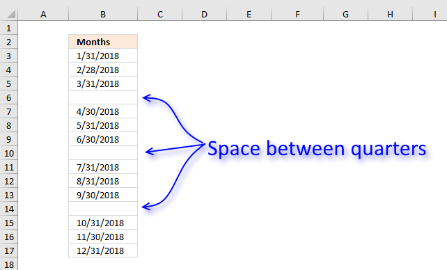
15. Create a list of dates with blanks between quarters
Answer:
Formula in B3:
If you don't need the formula to be dynamic, like in a dashboard or an interactive sheet then simply follow Jarek's instructions below.
Jarek comments:
- Create a list of 3 months in a quarter
- Select it together with a blank cell beneath
- Drag down
Thanks!
Explaining formula in cell B3
Step 1 - Check blank cells above
We want to know how many cells above have been populated with dates in order to calculate the next date.
$B$2:B2<>""
becomes
"Months"<> ""
and returns FALSE.
Step 2 - Sum values
The SUMPRODUCT function can't sum boolean values, we need to convert them into their numerical equivalents.
SUMPRODUCT(($B$2:B2<>"")*1)+1
becomes
SUMPRODUCT((FALSE)*1)+1
becomes
SUMPRODUCT(0)+1
becomes
0+1 and returns 1.
Step 3 - Create date
The DATE function creates an Excel date based on year, month and day.
DATE(2018, SUMPRODUCT(($B$2:B2<>"")*1)+1, 1)
becomes
DATE(2018, 1, 1)
and returns 43132.
Step 4 - Convert the Excel date to something we understand
The TEXT function can do many things, one of them is to format an Excel date.
TEXT(DATE(2018, SUMPRODUCT(($B$2:B2<>"")*1)+1, 1)-1, "M/D/YYYY")
becomes
TEXT(43132, "M/D/YYYY")
and returns 1/31/2018 in cell B3.
Step 5 - Create a blank between quarters
The IF function uses the logical expression to determine if a date or blank is to be returned.
IF(MOD(ROWS($A$1:A1), 4), TEXT(DATE(2018, SUMPRODUCT(($B$2:B2<>"")*1)+1, 1)-1, "M/D/YYYY"), "")
becomes
IF(MOD(ROWS($A$1:A1), 4), "1/31/2018", "")
The MOD function returns the remainder after a number is divided, this allows you to create a squency of values that repeats 1, 2, 3, 0, 1, 2,3, ... and so on.
IF(MOD(ROW(A1), 4), "1/31/2018", "")
becomes
IF(1, "1/31/2018", "")
and returns "1/31/2018" in cell B3.
Get Excel *.xlsx file
Create-a-list-of-dates-with-blanks-between-quarters.xlsx
16. Create a monthly date range
I will demonstrate three different techniques to build monthly date ranges, in this section. Two of these techniques are easy because they have the start and end date in a cell each.
To have two dates in the same cell makes it more complicated but I have a solution for that, as well.
16.1 Create date ranges using a built-in feature
To build a date range that begins with the first date in a month and ends with the last date in a month follow these steps:
- Type the start date of your first date range in one cell
- Type the end date of your first date range in the next cell
- Repeat above steps to enter the second date range in cells below
- Select all cells
- Press and hold on black dot
- Drag to cells below as far as needed
Excel dates are actually numbers, the above technique uses Excel's ability to quickly create number sequences using the selected cells as a guide to determine the size of the date ranges below.
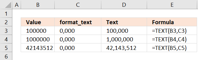
16.2 Basic formula
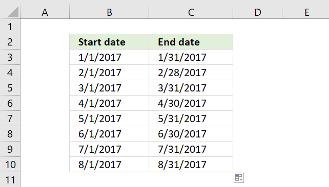
Type the start date in a cell, in this case, 1/1/2017. Type the following formula in the next cell:
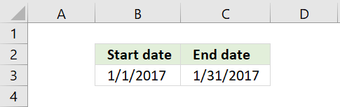
The formula in cell C3 calculates the last date for the month and year in cell B3. It actually calculates the first date in the next month and then subtracts with 1.
This solves the issue with some months having 30 days and some having 31 and February with 28 days in common years and 29 days in leap years.
The next date range has the first date in the next month as the start date. The formula is almost identical to the previous formula.
Formula in cell B4:
Now copy cell C3 and paste to cell C4.
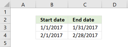
The relative cell references in the formula changes accordingly, you can read more about relative and absolute cell references here:
Recommended articles
What is a reference in Excel? Excel has an A1 reference style meaning columns are named letters A to XFD […]
Copy cell range B4:C4 and paste to cells below as far as needed.
16.3 Advanced formula
The following picture shows you date ranges in a single cell each. To get that you need to build a somewhat more complicated formula.

Formula in A4:
copied right as far as necessary. The TEXT function formats the number from the DATE function as a readable text string in a format you choose. You can read more about the TEXT function here:
Recommended articles
What is the TEXT function? The TEXT function is a helpful tool that allows you to change how a number […]
Formula in A7:
copied right as far as necessary.
Formula in A10:
copied down as far as necessary.
Formula in A19:
copied down as far as necessary.
16.4 Get *.xlsx file
Create a monthly date range.xlsx
Dates category
This article demonstrates how to return the latest date based on a condition using formulas or a Pivot Table. The […]
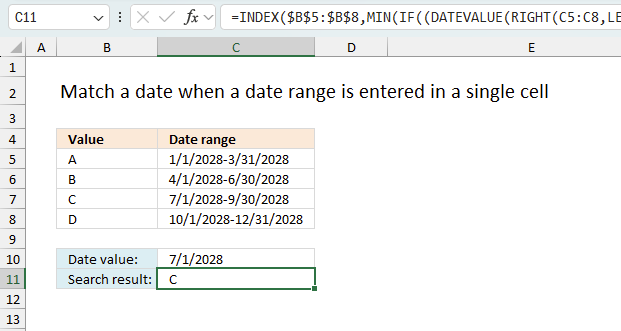
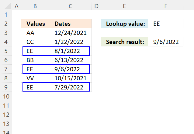
This article explains how to search for a specific date and identify a date range in which it falls between […]
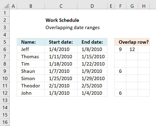
This article demonstrates a formula that points out row numbers of records that overlap the current record based on a […]
Dates basic formulas category
This article demonstrates how to return the latest date based on a condition using formulas or a Pivot Table. The […]
This article explains how to search for a specific date and identify a date range in which it falls between […]
Excel categories
183 Responses to “How to create date ranges in Excel”
Leave a Reply
How to comment
How to add a formula to your comment
<code>Insert your formula here.</code>
Convert less than and larger than signs
Use html character entities instead of less than and larger than signs.
< becomes < and > becomes >
How to add VBA code to your comment
[vb 1="vbnet" language=","]
Put your VBA code here.
[/vb]
How to add a picture to your comment:
Upload picture to postimage.org or imgur
Paste image link to your comment.
The question of exactly *why* you would want blank rows in your data remains unanswered.
I guess it would increase sheet readability in large lists.
I just try to solve peoples excel questions. If the solutions seem useful I post them here.
how can i get the date range as : 01/01/09 - 01/15/09, 01/16/09 - 01/31/09 and so on
=TEXT(DATE(2009, 1, 4)+(ROW(1:1)-1)*14, "mm/dd/yy")&"-"&TEXT(DATE(2009, 1, 4)+(ROW(1:1)-1)*14+13, "mm/dd/yy") + ENTER copied down as far as necessary.
Put your START date in BOTH spots that say (2009, 1, 4)...
Try this: =TEXT(IF(MOD(COLUMNS($A$1:A1), 2), DATE(2009, ROUND(COLUMNS($A$1:A1)/2, 0), 1), DATE(2009, ROUND(COLUMNS($A$1:A1)/2, 0), 16)), "MM/DD/YY")&"-"&TEXT(IF(MOD(COLUMNS($A$1:A1), 2), DATE(2009, ROUND(COLUMNS($A$1:A1)/2, 0), 15), DATE(2009, ROUND(COLUMNS($A$1:A1)/2, 0)+1, 1)-1), "MM/DD/YY") copied right as far as necessary.
I guess the formula can be done a lot smaller.
See this blog post: https://www.get-digital-help.com/create-a-custom-date-range-in-excel/
Here is a way to do it with shorter formulas, but you have to be willing to use only Column C's #NUM! error to identify when to stop looking (Column D's value will repeat the previous rows value at this location).
Put =A2 in cell C2, then put this array-entered** formula in C3 and copy it down...
=SMALL(IF(A$3:A$100-A$2:A$99>1,(A$3:A$100-A$2:A$99>1)*A$3:A$100),ROW(A1))
Next, put this array-entered** formula in D2 (note, this is D2, not D3) and copy it down...
=SMALL(IF(A$3:A$100-A$2:A$99>1,(A$3:A$100-A$2:A$99>1)*A$2:A$99,LOOKUP(2,1/(A$1:A$65535""),A:A)),ROW(A1))
The top ends of the offsetted ranges (A$99 and A$100) can be any cell address that is equal to or larger than the cell address of the last date.
**Commit this formula using Ctrl+Shift+Enter, not just Enter by itself
A follow up to my previous post...
The last paragraph (right before the double-asterisk note) does not read exactly right; perhaps this is better...
The top ends of the offsetted ranges (A$2:A$99 and A$3:A$100) can be any cell addresses, still offsetted by one, that is equal to or larger than the cell address of the last date. The key to keep in mind is the the number of cells in each of the two ranges must be the same because this is an array-entered formula and, as such, the iteration process inherent in an array-entered formula requires a cell-for-cell correspondence.
Very good, both formulas are shorter!
Thank you for your contribution and explanation!
Wow this is for the Excel Black belt guys!
Oscar for the benefit of those who aspire to get here someday, could you please explain in brief the logic and what part of the formula is doing what.......
chrisham,
Thanks!!
I will explain this post and all the others as soon as I can. This post is now number one on my update list.
this isn't working when i copy and paste?
clay,
There seems to have been a typo.
You may also need to adjust mm/dd/yy depending on your regional settings.
https://www.techonthenet.com/excel/formulas/text.php
Thanks for commenting!
why not simply create a list of 3 months in a quarter
then select it together with a blank cell benneath
then drag down
?
Jarek,
your answer to this question is the easiest one. Thanks for your contribution!
welcome, any time
;-)
credit to my boss - I once tried to show him a similar formula solution. he listened and presented me a solution of his own (as above). I was devastated.
;-)
Hey there! Awesome help!
I need something similar to this, however, with an added piece.
I need a formula that if I enter a start date in field B1 such as 6/8/11 it will give me the date ranges for 7 days in fields B3-B14. Does that make sense?
Basically I want a formula that will tell me when a client is admitted to services on 6/8/11, their week 1 is 6/8/11 to 6/15/11; week 2 is 6/16/11-6/22/11 etc through 12 weeks.
I want the initial date in B1 to be the only value that I have to change to produce these results. Is that possible?
Shannon,
read this post: Date ranges for 7 days in excel
Thank you for commenting!
Thanks! This is very helpful!
You are welcome!
Is there a way to reverse this formula to Convert date ranges into dates in excel. For example: from 1 March 2010 - 28 February 2011 to convert that in to list from A1 to A365 starting from 1 March 2010 and A2 2 March 2010 ans so on until 28 February 2011?
Tiaan,
read this post: Convert date ranges into dates in excel
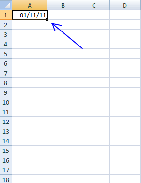
how do i get a range of date to show up.. in the first cell I want 1/11/11 and then each cell to follow the next date
example
b3 has 1/11/11 and then i want all 31 days to follow with out having to put each on in b4, b5, b6 and so on?
todd,
Press with right mouse button and hold on black dot.
Drag down and release right mouse button. Press with left mouse button on Fill series..
Hi I need help with a formula. Basically I have a date column and a true of false value column. What I need is a formula that says if the date in Column J is between 4/1/11-3/31/12 then enter 1 in Column M, if not enter 0 in Column M.
I hope you can help.
Thanks
Michelle,
Formula in cell M1:
perfect thank you Oscar
Michelle,
You are welcome!
Thank you!I used my extensive QA background to spot the use of a : and incorrect spacing in the formula for a6....Once again THANK YOU!
Here's what I ended up with
=TEXT(DATE(2011, 9, 19)+(COLUMNS($A:A)-1)*7, "mm/dd/yy")&"-"&TEXT(DATE(2011, 9, 19)+(COLUMNS($A:A)-1)*7+6, "mm/dd/yy")
DanL,
Thanks! I have updated this post.
I am trying to do a formula in excel 2003. It is quite complex.
The start date was June 13 and I need to reflect any blank cells that are 60 days out and any cells that are 91 days out.
The expirey dates are only for certain cells ($B$3:$F$3 and $N$3:$S$3).
Hope that makes sense :(
Richelle,
can you describe your question in greater detail?
Also add some example data and what you are trying to achieve?
Sure,
Employee Name- Company Start date - WHMIS - Orientation - H/R
John Smith - 17 Oct 11 - BLANK - 17 Oct 11 -BLANK
Johanne Smi - 16 Oct 11 - BLANK - BLANK -BLANK
I have an expirey date of 60 days (will be yellow in color after 60 days from the start date) and 91 days (will be red in color after 91 days from the start date). I only need the expirey dates for the Whimis and HR cells- the orientation cell does not require an expirey date.
I have tried this:
=today()-$b$12>60 and =today()-$b$12>91 and =today()-$b$12>59
that formala does not seem to work...
Richelle,
You are using absolute cell references in your conditional formatting formula.
You are also only using cell $b$12 when you say "I only need the expirey dates for the Whimis and HR cells". $b$12 is the company Start date?
you bet, $b$12 is the company start date. I am wanting the whole line to turn red/yellow when Whimis and HR are over due. The start dates are behind so I dont think (=TODAY)would work.
Richelle,
I am wanting the whole line to turn red/yellow when Whimis and HR are over due
In your example table, Whimis and HR are blank?
Employee Name- Company Start date - WHMIS - Orientation - H/R
John Smith - 17 Oct 11 - BLANK - 17 Oct 11 -BLANK
Johanne Smi - 16 Oct 11 - BLANK - BLANK -BLANK
WHIMIS and H/R are Blank.
Richelle,
Get the file:Richelle.xls
Not quite, when the dates are added it does not return to normal.
Dear Oscar
example: from 20/3/2000 to 31/10/2011 = 11.58, what is the formula i should use to get the result like this?
Richelle,
Get the Excel file: Richelle1.xls
You ROCK!
Thank you so much!
Shirley,
What are you trying to do?
Create dates with 11.58 years between them?
or
Calculate years between two dates?
Calculate years between two dates. :)
Shirley,
Is 0.58 a decimal fraction of a year?
I get 0.62 in my calculations.
Oscar,
I think yours is the correct one as i got 0.58 from my system which I found not accurate.
Shirley,
Formula in cell c4:
=TEXT(A4, "DD/MM/yyyy")&" to "&TEXT(B4, "DD/MM/yyyy")&" = "&ROUND((B4-A4)/365, 2)
This formula does not take leap years into account.
Excel dates: https://www.cpearson.com/excel/datetime.htm
thank you Oscar! i got the solution.
Dear Oscar,
I am really need your help in excel.
I want to sort some data in date between nov/1/2011 to nov/16/2011.this date is in column K.
what should I type the formula?
Thank you.
I have a question as well.
I have a column consisting of date, user, and another variable (lets call it food) on a sheet:
so ex.
A | B | C
-----------------------
Date | user2 | carrots
and it currently counts the number of times a user has eaten a food using the countifs function:
=COUNTIFS(Sheet2!B2:B9000,"=user1",Sheet2!C2:C9000,"=peas")
...this works perfectly.
The problem Im having is that I want to create another sheet where you can enter a date range and have it display only the results in that range, including the dates.
Any suggestions/help would be appreciated.
Came up with a solution - make a true/false date range column and pulled the data from that. Thanks anyway, learned a lot!
How can I create a data range for different data apart from dates- say personnel ID #s? the formula given here is for dates..
need to truncate the undermentioned column to create columns of weeks it has, for eg. 1/26/2011 was a wed, so need a column for 1/26/2011-sun 1/29/2011, and then onwards each week starting monday till 8/31/2011. please help asap
Assigned Dates
1/26/2011 - 8/31/2011
2/1/2011 - 3/30/2011
2/1/2011 - 3/30/2011
2/1/2011 - 3/30/2011
11/1/2010 - 2/11/2011
1/26/2011 - 8/31/2011
Ian,
Can you give me some examples of what you want to achieve?
Hi Oscar,
First of all, helpful blog!
May I ask here regarding finding the correct value based on and within the date range?
For example, column A contains all the different dates like (not arranged or sorted):
(1) 1/10/2011
(2) 23/3/2012
(3) 20/12/2011
(4) 3/1/2012
Reference list:
In column C, contains the expiration dates with corresponding values in column D.
For example (chronologically arranged):
31/05/2010 100,000.00
31/08/2010 200,000.99
30/11/2010 300,000.88
28/02/2011 400,000.77
31/05/2011 500,000.66
31/08/2011 600,000.55
30/11/2011 700,000.44
29/02/2012 800,000.33
25/03/2012 900,000.22
The Result (based on and before the date in Column C but the value in Column D):
(1) 1/10/2011 400,000.77
(2) 23/3/2012 800,000.33
(3) 20/12/2011 700,000.44
(4) 3/1/2012 800,000.33
Thanks for your time,
- oui
Hi Oscar,
Kindly disregard my previous message.
I think I've got it.
I've used LOOKUP function.
Thanks though,
- oui
I have a weekly report for work I use. My template needs to have the date formatted across one of the upper rows. I need it to read. January 2-6, 2012.
Thanks,
Matt
Deeks,
read this post: Filter weeks from a date range
Here is a solution to oui´s question:
Learn more: Return value if in range in excel
Matt,
That is not an easy question! I think you have to change formatting for each date.
Example,
Value in cell A1: 40910
1. Select cell A1
2. Press Ctrl + 1
3. Go to tab "Number"
4. Select custom in category
5. Type MMMM D-"6, " yyyy
6. Press with left mouse button on the OK button
Hi, Oscar! I went through all the Q and As, but not sure my question is answered. It's actually quite simple.
I need a date range, pulling the date from one column.
Column I:
DATE
17-Jun-11
Column J:
Date range (7 days after date in Column I to 21 days after date in Column I).
Further, is there any way to put into column K whether or not the date is out of the range, with a Y/N, or other means to denote out of range date?
THANKS for your help, IN advance!-Ingrid
Ingrid,
Date in cell I2: 17-Jun-11
Formula in cell J2:
This is awesome! THANK YOU!-ij
Hi Oscar, I'm looking for help in Excel.
In one column, I've dates for few years. I would like to have a column next to it which shows the corresponding Weeks, like Week1, Week2,...till Week5. Can you please help me with this?
Chaks,
I hope you´ll find an answer here:
https://www.rondebruin.nl/weeknumber.htm
or here:
https://www.cpearson.com/excel/WeekNumbers.aspx
When does week1 begin? There are few possible ways to number weeks. See links.
Hi Oscar, I need some help for excel.
I have 1 column containing the 365 days of 2010 written in short date like 01/01/2010. Then I have a second column with some cells containing data and some others left blank.
I want a formula that will write 1 if at least 50% of cells for a given month are fill and leave a blank cell if not. I want this formula to be aware of the month shift and easy to drag so that I will only get 12 values for a year.
I think this is impossible but you are the pro.
Ricardo,
It is possible!
Get the Excel file:
Ricardo.xls
Hello Oscar,
I am working with your date range formula from this post (Create a date range using excel formula). I am using the formula from A9, which includes ROW in the formula. Because all of the other cells in those rows are empty I get error warnings. Is there a way to avoid the error warnings regarding empty cells?
Many thanks.
Chaks
use this:
=INT((DAY(cell reference containing your date)-1)/7)+1
Chaks,
Correction!
Use this if you want to consider sunday as the first day of the week:
=INT((13-WEEKDAY(cell reference containing your date)+DAY(cell reference containing your date))/7)
the first formula would only consider the value of the days, and is not what you were looking for I think...
Flyingwater,
I am working with your date range formula from this post (Create a date range using excel formula). I am using the formula from A9, which includes ROW in the formula. Because all of the other cells in those rows are empty I get error warnings. Is there a way to avoid the error warnings regarding empty cells?
Formula in cell A9:
I don´t think ROW function is the problem here, maybe the "mm/dd/yy" gives you trouble?
I am trying a formula which gives me the month between dates what fall between 2 months. For example, 21/02/2012 - 20/03/2012 should return March
Adiel,
What if the date range is 21/02/2012 - 20/04/2012?
I am trying to get the date range that was used in a previous query to show up on the front page of my report. The Date range is selected by the user after running the Macro. I want that date range to be listed so when you run the Report you can visually see what date range was pulled. Lets say the Query name was Query1 and the field name was Field2. Oscar, Any idea?
Thanks!
Hi Oscar
I am specifically look at 21st of the month to 20th of the next month only. is it is 21/02/2012 - 20/04/2012 it should return an error.
Daniel,
Hard to say without seeing your workbook.
Adiel,
Is 21/02/2012 in one cell and 20/03/2012 in a different cell?
I have a spreadsheet that needs to report the number of days a certain document is over 3 shift days. Where I work is a 9 on and 5 off schedule and I need to exclude any of the days off so that the over 3 is actually only over 3 work days. I am thinking the NETWROKDAYS function may be used for this but can you help with this??
Glenn,
Can you provide some example data and what you want to achieve?
Добрый день, Оскар. Помогите решить проблему. Уже который день мучаюсь и все никак не получается посчитать.
Файл с данными я залил на обменник (mail.ru), вот ссылка, чтобы Вы сразу все увидели и поняли мои замыслы
https://files.mail.ru/CJAX0S
Мне необходимо посчитать сумму получившихся цифр за каждый месяц. Хочу задать формулу, которая находит из столбца "А" все даты относящиеся к нужному месяцу и посчитать сумму цифр из столбца "К". Строки в месяце могут добавляться и убираться, следовательно количество цифр изменяется и каждый раз пересчитывать - жутко неудобно.
Для примера покажите на одной цифре - сумма данных за февраль 2012.
Результат находится в L23.
Снизу ТАБ и справа вверху есть разные варианты формул, которые я пытался составить, но так ни одна и не заработала.
Заранее СПАСИБО! )))
Re Сергей, it could be translated as:
Hello, Oscar. Help me solve this problem. I am tormented day after day, and still can not get to "count".
Data file, I filled in the exchanger (mail.ru), here is a link for you to understand all of my designs
"link to his file"
I need to calculate the amount of the resulting figures for each month. I want to set a formula that finds the column "A" all dates relating to the desired month and calculate the sum of numbers in column "K". Rows can be added in the month to get out and therefore the number of digits is changed each time to count - terribly "uncomfortable".
For example, show one figure - the amount of data for February 2012.
The result is in L23.
Bottom-TAB and right at the top there are different versions of the formulas I have tried to make, but no one and did not work.
Thanks in advance! )))
Hi Oscar,
I'm hoping you can help me with my formula question. I have a schedule that I am working with and based on one date (ie. 6/4/12) different processes take different times to complete (ie. one step could only take a week, another could take up to 4 weeks). Is there a formula I can use to calculate each step in the process based off of the date range of completion for the first step in the process?
Let me know if you need more information.
Dear Oscar,
Thanks for the last post, I'm rely grateful for your help. I have another query regarding date format.
I have an excel sheet showing date as 11-08-2018, BUT
I want to convert this date FORMAT to 18-08-2011.
Your help in this matter shall be highly appreciated.
Cheers!
Danielle,
Your question seems interesting but I am not sure I fully understand. Can you provide an example?
Muhammad Nadeem Bhatti,
I am not sure how to solve it, try google:
excel yy/mm/dd dd/mm/yy
Sure! (Sorry i couldn't figure out how to paste this as an excel sheet)
So for example, if you look at the BBD date at the bottom, all of the steps above it take a certain amount of time to complete and have to be finished on time in order for the project to be complete by 1/4/2013. Instead of typing in manually the date ranges I am trying to write a formula that will allow me to input the project date (ie 1/4/2013) and have all of the other steps populate themselves based on how long they take to complete (ie. the manuscript to CE step could take 2 weeks, the manuscript from CE could take 1 week and so on). I hope that makes sense??
ie. ONE ROUND From: To:
Manuscript turnover 6/25/2012 7/30/2012
Manuscript to CE 8/6/2012
Manuscript from CE 8/20/2012
Manuscript to author 8/27/2012
Manuscript from author 9/10/2012
Ms to comp 9/3/2012 9/17/2012
Pages from comp 10/8/2012
Pages from author 10/22/2012
Pages to proofreader 10/29/2012
Pages from proofreader 11/12/2012
Pages to comp 11/19/2012
Confirming proofs 11/26/2012
Ship to printer 12/3/2012
BBD 1/4/2013
Danielle,
read this post:
Calculate dates in each step in a project based on a finish date
Thanks! I posted my comment under the other link!
Hi,
The above formula in A9 "Increasing date in a column" works pretty good however I have a small request to change the formula as per my need.
As I fill the first column in excel with this formula than use + handler on bottom right of the column to drag and copy it to next cell so the date increases. That works but when it reaches the end of month it continues in the same cell. Is it possible so at the end of the month the range would stay within the month instead of increasing to next month?
Here let me try to explain visually.
01/01/12-01/07/12
01/08/12-01/14/12
01/15/12-01/21/12
01/22/12-01/28/12
01/29/12-02/04/12 <-- can this be 01/29/12-01/31/12 ?
And next month would be per week in each coulmn as well and so on.
02/01/12-02/04/12
02/05/12-02/11/12
02/12/12-02/18/12
02/19/12-02/25/12
02/26/12-02/29/12
03/01/12-03/03/12
Thank you.
Anees,
Your question is really complicated and I like that. But unfortunately I don´t have an answer right now.
I have the exact same question as Anees and I was just wondering if you have found a solution. Thanks
Anees and charles,
Read this post:
Date ranges: Weeks within a month
hey oscar ... i used the date range formula in your A3 example above. it's great! thanks! now i'm trying to reference these dates ranges in a sumifs statement. for example (if i can do this) ... my current formula is:
=SUMIFS('PO LOG'!$L$5:$L$1036,'PO LOG'!$K$5:$K$1036,SUMMARY!A10,'PO LOG'!$J$5:$J$1036,SUMMARY!D$3)
'PO LOG'!$L$5:$L$1036: column L lists invoice dollars amounts
'PO LOG'!$K$5:$K$1036: column K lists expense codes
SUMMARY!A10: individual expense code
'PO LOG'!$J$5:$J$1036: column J list invoice dates
SUMMARY!D$3: date range created from your A3 formula above (ex: 02/19/12-02/25/12)
this formula is returning zero dollar amounts - which obviously isn't correct. however, i'm not getting an error with the formula. any help you can give would be amazing! thanks so much.
best ... josh
Josh,
Try this formula:
=SUMIFS('PO LOG'!$L$5:$L$1036,'PO LOG'!$K$5:$K$1036,SUMMARY!A10,'PO LOG'!$J$5:$J$1036,"<="&RIGHT(SUMMARY!D$3, LEN(SUMMARY!D$3)-SEARCH("-", SUMMARY!D$3)),'PO LOG'!$J$5:$J$1036,">="&LEFT(SUMMARY!D$3, SEARCH("-", SUMMARY!D$3)-1))
Hi Oscar, im just trying to change the format from 09/02/2012 to 2 Sept is it possible, ive tried format with no luck whatsoever, it just doesnt seem to take any change, even tried to change it to a percentage still no effect. looks like the formula is locked in a format style?
Osman,
Change the formula from "mm/dd/yy" to "dd mmm".
Example formula in cell A3:
=TEXT(DATE(2009, 1, 4)+(COLUMNS($A:A)-1)*7, "dd mmm")&"-"&TEXT(DATE(2009, 1, 4)+(COLUMNS($A:A)-1)*7+6, "dd mmm")
Hi Oscar,
I’m trying to create a date range in an excel calendar. I’ve got the calendar to update to whatever year you type in so that it can be used to check past/future appointments and events, and I’ve got one sheet that shows important events and the dates they occur – when you add to the list it then updates the calendar to show that event.
What I’m having trouble with is showing a week-long event, e.g.: instead of the date being 23/10/2012, the relevant cell on the events sheet would show 23/10/2012-27/10/2012 AND this being updated on the calendar sheet to show the event covering multiple days.
I got a friend to help me with most of the formulas for this, so I’m having trouble working this problem out for myself! I think if I knew how to do the date range to show in a single cell, I might be able to work out how to get it to update the calendar (though if you have any ideas on this as well that would be great!)
Any help would be really appreciated.
Thanks
Green,
Formula in cell E1:
=IF((DATEVALUE(LEFT($A$1, FIND("/", $A$1)-1))<=D1)*(DATEVALUE(RIGHT($A$1, LEN($A$1)-FIND("/", $A$1)))>=D1), $B$1, "")
Hi Oscar
I need your assistance in putting together a formula to show a period of time between two dates. For example:
09/02/1990 to 04/03/2000 to say 10 years 24 days
If the dates have months included then I need t show that as well. We use this to identify periods to credit as experience.
Much appreciated
Cyril
Hi Cyril, why don't you use datedif? such as :
If date start in A1 and date end in B1 then in C1 type:
=DATEDIF(A1,B1,"y")&" years "&DATEDIF(A1,B1,"ym")&" mos "&DATEDIF(A1,B1,"md")&"days"
Would that work for you?
Hi Oscar
Yes this is exactly what I need. Just another piece to add, how do I total several periods with dates formatted like this, I can't just use a SUM formula (I tried). For example:
10 years 2 months 24 days plus
2 years 0 months 16 days
This would be 12 years 3 months and 0 days.
Please advise and your assistance is very much appreciated.
Cyril
Hi Cyril Clarke,
This is cyril not Oscar, for sure Oscar will have a solution that may be far more elegant. As for your query based on my proposed solution, DATEDIF would work with two (2) strings. A date to start and a date to end.
This may not work in your case if the two sets of periods are separated by another period that should not be computed. (hope I make sense).
Or you could use SUMPRODUCT(DATEDIF(RANGE_START,RANGE_END,"y")) ... such as =SUMPRODUCT(DATEDIF(A1:A2,B1:B2,"y"))
Would that work for you?
Hi Cyril
No this formula did not work but it is close as it has returned a zero rather than N/A so there may just be a tweak required.
Also I noticed above that my example shows as:
10 years 2 months 24 days plus
2 years 0 months 16 days
This would be 12 years 3 months and 0 days.
This should actually be 12 years 3 months and 10 days.
Apologies
Cyril
Understood, kindly type:
=DATEDIF(A1,A1+((B2-A2)+(B1-A1)),"y")&" years "&DATEDIF(A1,A1+((B2-A2)+(B1-A1)),"ym")&" month "&DATEDIF(A1,A1+((B2-A2)+(B1-A1)),"md")&" day
that is with data as follows:
2/9/90 5/3/00
2/5/01 2/21/03
In A1 Start First date
In B1 End First date
In A2 Start Second date
in B2 End Second date
this will give you:
12 years 3 month 10 days
would that work for you?
forgot a " after the word day...
Hi Cyril
This is exactly what I needed and is rather eloquent. I have now put in the cells numbers that I need and it is giving me the result I would have expected. I had noticed the missing rabbits ears. It is unusual to be dealing with someone who has the same name as me, it is not a common name.
Thank you very much
Cyril
Glad it worked for you.
Cheers!
Hey guys,
So I have a spreadsheet where each row is a purchase including the Date (year, Month, Day) and cost (along with other variables). I have another table that includes dates that I received paychecks. What I want to do is create a table that sums the spendings in between paychecks.
Thanks!
Figured it out with some crazy codes, this page was extremely helpful! Thanks to all!
Any ideas why - if I enter 20/7/12 to 30/7/12 the range is expanded from 24/7/12 to 30/7/12 (and does not start at the 20th)?
resolved - not sure what the problem was though
How would you modify the formula for just weekdays? So you would have a 5 day range instead of 7 and the next column skips the weekend and starts on the following monday.
Ryan,
Formula in cell A1:
Copy cel A1 and paste down as far as needed.
Hi Oscar
I have an issue which is not related to dates. I need assistance where if a value exists in a cell in my spreadsheet then the cell I am in should return a zero value. I have several values that are conditional on there being a zero in another cell.
We use these variables for moving people from one part of the country to another. For example, a teacher's kids stay in their former location while the teacher finds permanent housing they get one payment whereas if they move with them they get a different payment.
Please advise.
Thanks
Cyril
Re: if a value exists in a cell in my spreadsheet then the cell I am in should return a zero value
Why not using some such as =IF(AB10<>0,0,"EMPTY")
Not knowing the cell reference, just replace AB!) with the cell of reference and "N" with whatever you want in cell is empty.
haaaa, wrap code... formula is =IF(AB10<>0,0,"EMPTY")
less than more than... hopefully Oscar can edit and delete redundant posts...
I am not sure I got less than and more than where you wanted them?
Thanks Oscar.
that is correct. will return a zero if a value (that is equal to zero) exist in the cell, will return "empty", for empty cell and zero values.
Hi Oscar,
I am facing a small problem as follows :
Column A has 12 items with their quantities mentioned. Column B has 14 items with their quantities mentioned.
There are two items in column B that are not in column A and two items in column A not in the other one.
The objective is to merge the two columns without having repetition of any item in the merged column.Once I have this, I want to sum up the quantities of each items from the two columns and show next to the items in the merged column.
Please advise.
Many Thanks
Haroun
Haroun,
1. Put the quantities in separate columns. Perhaps you can do this by using "Text to columns"?
2. Filter unique distinct values from the two columns combined:
https://www.get-digital-help.com/extract-an-unique-distinct-list-from-two-columns-using-excel-2007-array-formula/
3. Use two Sumif functions to sum up quantities of each item from the two columns.
A pivot table can do all this almost automatically if you combine both lists before creating the pivot table.
https://peltiertech.com/Excel/Pivots/pivottables.htm
Hi Oscar,
Need help with a formula Please. I need to figure out the date range of a cell. So if cell "E2" has a date of 11/23/2012 then that would need to fall under date range of "11/19 - 11/25". I have the following date range I need to identify: "11/12 - 11/18", "11/19 - 11/25", "11/26 - 12/2", "12/3 - 12/9", "12/10 - 12/16", "12/17 - 12/23", "12/24 - 1/1/2013". I tried the formula below but I keep getting a result of "False". I appreciate any help I can get. Thank you
=IF(E2<11/18/12,"11/12 - 11/18",IF(E2<11/25/12,"11/19 - 11/25",IF(E2<12/2/12,"11/26 - 12/2")))
Elizabeth,
read post: Find date range
[...] in Dates, Excel, Search/Lookup on Nov.22, 2012. Email This article to a Friend Elizabeth asks:Hi Oscar, Need help with a formula Please. I need to figure out the date range of a cell. So if cell [...]
Hi Oscar,
I have a question regarding creating a table based on a date range. Say I had a date range (11/27/2012 through 9/27/2033) and I wanted the endpoints to be adjustable. Is there a function I could use, like a PivotTable, to make that happen?
Thanks,
Nate
Nate,
Can you explain in greater detail?
I am trying to count Camper Nights in an RV park, by electric service dates. For Example, a RV camp reserved a pull thru with arrival date of 6/1/12, next column has departure date as 8/15/12. The electric service date (on electric bill) are 6/24/12-7/21/12, 7/22/12-8/23/12. So, I need to count how many camper night fall within each billing cycle. Can you help?
Mr. Oscar,
I have a question.
Cell A1 is haveing date say 01/08/2013
Cell A2 is having no of days say 33 days
Cell A3 is having end date i.e 11/09/2013 by using WORKDAY.INTL(A1,A2,16,$BA$1:$B$10)function.
I need to have the new value in cell a3 every after 33 days(11/09/2013) automatically)
kindly advise
*I need to have the new value in cell a1 every after 33 days(11/09/2013) automatically)
Dear
How can I change the formula, inserting blanks between each group :
(no macro please, shared file, users forget to enable macro's)
link to image :
https://s24.postimg.org/smz0khqc5/Blank_between_groups.jpg
Thanks for your help
Oliver
I think you may have covered this at some point, but I can't seem to get the dates to change appearance as I need them to.
What this formula creates is a date that looks like this: 09/23/2013
However, I only want the month and date to be displayed like this 09/23
I need to show 12 weeks of dates so having the whole date takes up too much room.
I have tried changing the displayed value using conditional formatting and the trick you showed Matt in an earlier post, but the look of the dats never changes.
Is this possible?
Heya, your awesome!!! thanks a lot for posting this up. It saved me alooot of time
Cheers,
sandy
How can I have a formula for this:
Column A: Week of 09/30 to 10/04
Column B: Week of 10/07 to 10/11
Column C: Week of 10/14 to 10/18
Column D: Week of 10/20 to 10/24
Thanks for your help
JAH
Hi Oscar,
I am a beginner with excel so my question it might be simply-answered. I m trying to make a graph with the fluctuation of the rates during the year. I have periods in column A and rates in Column B. How can I set date ranges with constant rates? (e.g. from 01/01/2013 to 05/01/2013 $100)?
Thanks,
Dennis
Thanks for your help, I manage to have what I needed but I want the First cell to Automatically change each monday to the new date (Between Monday and Friday). I also Need to have the Phrase "Week of" before the date.
12/09/13-12/13/13 12/16/13-12/20/13 12/23/13-12/27/13 12/30/13-01/03/14
Thanks again
JAH
How do I create a function that will take the date range I enter and continue with it? for example, if I enter, "12/30/13-01/05/14" in cell a3, I want a4 to have, "01/06/14-01/12/14" and so on down the column.. Any and all help would be greatly appreciated!
Hello, I need to return data to a report from a master sheet by date range
Master sheet has several columns, one of which contains timestamps, I need the report sheet to return the data in another column of the row, based on the date range. I can make the timestamps be in the first column if it's easier.
Can you assist please
Hi,
I tried coping and pasting the formula out of Cell A9 to my spreadsheet and got an error msg as follows #VALUE!
Please Help!!!!!!!!!!!!!!!!!!!!!!!!
Matt,
1. Select a #VALUE cell
2. Go to tab "Formulas"
3. Press with left mouse button on "Evaluate formula" button
4. Check what part of the formula is giving you an error.
What is giving you an error?
Hi Oscar sorry for the late reply didn't realise you had responded, the error I am getting is actually #NAME? and the evaluation revealed that the error was in "(DATE(2009, 1, 4)"
It ok i just worked it out i was copying and pasting the "ENTER" into the formula my bad
Now i have another problem, i cant adjust the dates, im trying to enter 15/04/2015 in the format dd/mm/yyyy but it just wont commit.
Very helpful. I'm at a novice level on most of Office products but I seem to muddle through alright. This got me through so I could copy/paste the date range I wanted.
I was looking for the same thing Andrew (above) referred to but this worked wonderfully. Thanks!
Hi, sir i'd like you to help me about the formula to show the date after a period day. Ex. i have a meeting on 22/04/2015 and i'll have a meeting again after 21 days so i want to know the date will be on.
thank
Puthea
Enter this formula: =DATE(2015,4,22)+21
thank you Oscar i try it now
HI Oscar
Thank you for your help.
I am looking to create a formula that highlights a cell in red if the invoice date + 91 days is after today.
=if(TODAY>L114+91)then RED
It must also keep the L114+91 (example) Date in the cell
I hope thats clear
James
James
Try this conditional formatting formula:
=L114>TODAY()+91
Hi Oscar sorry for the late reply didn't realise you had responded, the error I am getting is actually #NAME? and the evaluation revealed that the error was in "(DATE(2009, 1, 4)"
Hi, I want to only mention Start & End date in Cell C9 & C10 respectively. Based on this workdays calculated I want to display all dates between Start/ End date in a row.
For Example: Start Date = 19 May 2015, End Date = 23 May 2015, WorkDays = 4
Then in row 4, I want to display 20 May, 21 May, 22 May. 23 May starting form F4 cell. I also want to exclude Saturday and Sunday if they are falling between Start & End Date.
Hi oscar.. Can you give me a formula to calculate a starting date to present and the result would be in how many years months and day. Example start on january 1, 2015 and today is feb 2,2015 the result would be 0-year, 1-month, 2-days
Sherwin,
Take a look at this:
https://excelsemipro.com/2011/01/how-many-years-months-and-days-has-it-been/
Hi Oscar, I need the First cell to Automatically change each monday to the new date (Between Monday and Friday). I also Need to have the Phrase "Week of" before the date.
12/09/13-12/13/13 12/16/13-12/20/13 12/23/13-12/27/13 12/30/13-01/03/14
How can I do this?.
Thanks
JAH
Hi can you create a formula where if the payment end dates fall within the following date range:
from the 1st through the 7th day of the month;
from the 8th through the 14th day of the month;
from the 15th through the 21st day of the month;
from the 22nd through the last day of the month.
that the CRA remittance is due on the 3rd working day excluding Sat, Sun and stats below:
1-Jan-2016
8-Feb-2016
25-Mar-2016
28-Mar-2016
23-May-2016
1-Jul-2016
1-Aug-2016
5-Sep-2016
10-Oct-2016
11-Nov-2016
26-Dec-2016
27-Dec-2016
Hi..............
Sir, my question is???
My Product Name - Samsung-E1200 just time price - 1120/-
and then price drop it this product - Samsung-E1200 - 1175/-
so sir howes condition apply i m not understand????
so sir please suggest me............. and question is ????
01-feb to 14-feb price 1120/-
then 15-feb to 29-feb- price change 1175/-
so suggest me???????
I want a help from you in excel
hi Oscar,
I am stuck on an excel problem.
I have thousands of cells of data.
In one column I have manually entered dates. Sometimes the date is a single day (1/1/2003). Other times it is a manually entered date range (1/1/2003-5/1/2003). A few columns later each entry has a numerical value to capture the scale of something I am measuring. The numbers are like: 10, 126, 480; and so on.
Elsewhere in the spread sheet I want to return a single value for the sum of all the numbers that correspond to a specific date, So for example,
TAB 1
DATE VALUE
1/1/2003 20
1/1/2003-5/1/2003 10 (i.e. 10 per day)
1/1/2003-20/6/2007 10 (i.e. 10 per day)
and so on....
TAB 2
DATE VALUE (I need the formula to calculate below)
1/1/2003 40
2/1/2003 20
3/1/2003 20
4/1/2003 20
5/1/2003 20
6/1/2003 10
Is that clear?
Can you help me with that?
ben
ben,
Array formula in cell B8:
=SUM(IF((A8>=$A$2:$A$5)*(A8<=$B$2:$B$5),$C$2:$C$5,""))
Hi Oscar,
Nice formula, I used the Row 3 format - =TEXT(IF(MOD(XXX formula, but need your assistance for getting this working on my computer; when I copy paste the formula it, works for the first cell only,as the gap I am trying to achieve is 7 days, but when I drag the formula to adjacent column, the gap incrases to 16 days. Can you suggest a fix for this please?
I tweaked the formula as below, but needs refinement from an expert like yourself
=TEXT(IF(MOD(COLUMNS($I$5:I5),2), DATE(2016,ROUND(COLUMNS($I$5:I5)/2,0), 1),DATE(2016,ROUND(COLUMNS($I$5:I5)/2, 0),7)),"DD/MM/YY")&" - "&TEXT(IF(MOD(COLUMNS($I$5:I5),2), DATE(2016,ROUND(COLUMNS($I$5:I5)/2,0), 7),DATE(2016,ROUND(COLUMNS($I$5:I5)/2, 0)+1,1)-1),"DD/MM/YY")
Trying to achieve 01/01/16-7/01/16, 8/01/16-15/01/16, using dd/mm/yy format.
Thanks,
Nav
Nav
Is this what you are looking for?
=TEXT(DATE(2016, 1, 1)+(ROW(1:1)-1)*7, "mm/dd/yy")&"-"&TEXT(DATE(2016, 1, 1)+(ROW(1:1)-1)*7+6, "mm/dd/yy")
Hi Oscar! How are you? First of all I'd like to tell you how admire your work and the dedication you put in it till these days.
I've tried to duplicate the A3 formula in GOOGLE SPREADSHEET - but no success.
Could you help me?
Thank's already pal
Hi Oscar,
I'm trying to make a weekly candlestick chart for my retirement fund's daily share prices. I can make such a chart but the values have to be arranged as ...
A B C D E
Date Open High Low Close
My problem is that the info is in a csv file and when I open it the data is arranged as ...
A B
Date Price
So is there a way to programmatically rearrange the later to the former?
Thanks in advance,
Eric
Eric
To my knowledge, you cant extract the open, high, or low out of a closing price. You source data needs to be in greater detail.
Hi,
I'm trying to get the formula to generate this:
June 24 - July 6
July 7 - July 20
July 21 - August 3
August 4 - August 17
August 18 – August 31
September 1 - September 14
September 15- September 28
September 29 - October 12
October 13 – October 26
October 27 - November 9
November 10 - November 23
November 24 - December 7
December 8 - December 21
December 22 - January 4
January 5 - January 18
January 19 - February 1
February 2 - February 15
February 16 - March 1
March 2 - March 15
March 16– March 29
March 30 - April 12
April 13 – April 26
April 27 - May 10
May 11 - May 24
May 25 - June 7
June 8 - June 23
Note that all ranges are 14 days, but the first and last date ranges are not 14 days.
Please help. I can figure out the end date
Spence, is there some logic in that sequence? I know 14 days but that doesn't help much.
Do you want a formula so you simply can provide a start date and the formula does the rest or how will it work?
Oscar,
I would like to add an empty row between each date range but excel seems to lose the formula when I do. It will start to skip weeks in the sequence. Can you help?
Devon,
This regular formula seems to work:
=IF(MOD(ROWS($A$1:A1), 2), TEXT(DATE(2009, 1, 4)+(INT(ROW(2:2)/2)-1)*7, "mm/dd/yy")&"-"&TEXT(DATE(2009, 1, 4)+(INT(ROW(2:2)/2)-1)*7+6, "mm/dd/yy"), "")
[…] got this from Carol Weideman, thank you! I think it is really simple and […]
hi
How to set date range like
1 Jun 18 in first cloume
formula for calculate 7+4 days
and how to set error If date less then 7 days and more then 11 days
Hi
I have this formula (=SUMIFS($C$14:$C$1000,$A$14:$A$1000,">="&DATE($A$1,8,1),$A$14:$A$1000,"<"&DATE($A$1,9,1),$F$14:$F$1000,$AA1)) which works but I want it to show from the 4th Sunday of a month to the 4th Sunday of the next month.
Thank You
Alan
Hi Alan,
I have added your question and an answer to this article:
https://www.get-digital-help.com/excels-sumifs-function-explained/
I have "1/1/2020" in Cell B1. I need to have a date range to show a follow-up appointment scheduled for 1 year in the future +/- 60 days from the date Displayed in cell B2 (i.e. 11/01/2020 - 03/01/2021). How can I do that?
Function daterange(targetbegin As Range, targetend As Range, Optional VolatileParameter As Variant) As VariantDim begindate As Date
Dim enddate As Date
begindate = targetbegin.Value
enddate = targetend.Value
daterange = begindate & " - " & enddate
End Function
in the formula bar: =daterange(startcell, endcell, NOW())
Hi,
How can I get the date change automatically from another cell in the same spreadsheet? For instance, I typed in today's date, 23 Jun in Cell A2 and I want the dates changed in Cell A38, A74, A110 and A146 just by changing the date in Cell A2.
Cheerio,
Ida
Hi,
Anybody could help me about Due Dates of an Amortization to get the output every 7th and 22nd of the month.
Example:
If a member borrow a money on June 22 - June 30 the due dates will be
July 7
July 22
August 7
If a member borrow a money on July 7 - July 15 the due dates will be
July 22
August 7
August 22
Thanks in Advance
THANK YOU THANK YOU THANK YOU !!!
I want a excel formula to calculate date range increment by the day.
So say i input 01/03/2021 as my start date.
Today is 26/03/2021 the new column should return 26 days.
sort of days counter
How would I simply extrapolate a date range in ONE column BY QUARTER? I would like to start on any given day and drag the right side of the cell and it increase the date by Quarters...not days, weeks, months or years--Quarters.
Stunned at how difficult it has been to find the solution to this.
Your way above I suppose will allow me to accomplish what I want, but with extra steps/info I do not need.
I hope I've explained this clearly enough.
Why won't Excel simply put "Quarter" as an option in the date range extension already in the product?
I look forward to your wisdom.
Thanx
Cheers!
Wouldn't be easier to use new 365 functions?
JohnH,
Yes, of course. Thank you for telling me, I will update this.
Need formula, which does not require dragging, to return a list of n dates that are n months apart from a given date. Hence, list of n Certificate of Deposit (CD) dates that are n months apart. Example, list of 5 dates that are 3 months apart from 2/24/2024 is:5/24/2024, 8/24/2024, 11/24/2024, 2/24/2025, and 5/24/2024.
I tried using SEQUENCE but cannot determine how to set STEP by n months.
Thank you!
Cal,
try this formula:
=DATE(2024,2+{3;6;9;12;15},24)