Fuzzy VLOOKUP
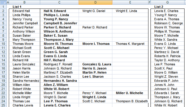
Table of contents
1. Fuzzy VLOOKUP - Excel 365 LAMBDA function

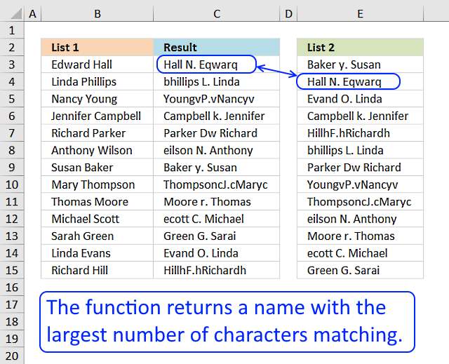
The image above shows a formula in cell D3 that extracts three values from column H (List2) that has as many matching characters as possible with the value in cell B3. The SEARCH function finds the characters, however, it has a limitation. It finds only the first character searching from left to right in a string. This means that repeated duplicate characters are also found when they might not be there.
The formula in this post doesn't have this counting issue:
Fuzzy lookups - Excel 365 recursive LAMBDA function
It is more accurate than the formula demonstrated here.
Excl 365 formula in cell D3:
Explaining formula
Step 1 - Count characters in cell B3
The LEN function returns the number of characters in a cell value.
Function syntax: LEN(text)
LEN(B3)
Step 2 - Create a sequence from 1 to LEN(B3) arranged horizontally
The SEQUENCE function creates a list of sequential numbers.
Function syntax: SEQUENCE(rows, [columns], [start], [step])
SEQUENCE(,LEN(B3))
Step 3 - Split characters
The MID function returns a substring from a string based on the starting position and the number of characters you want to extract.
Function syntax: MID(text, start_num, num_chars)
MID(B3,SEQUENCE(,LEN(B3)),1)
Step 4 - Search characters in $H$3:$H$101
The SEARCH function returns the number of the character at which a specific character or text string is found reading left to right (not case-sensitive)
Function syntax: SEARCH(find_text,within_text, [start_num])
SEARCH(MID(B3,SEQUENCE(,LEN(B3)),1),$H$3:$H$101)
Step 5 - Count numbers in variable a
The COUNT function counts all numerical values in an argument.
Function syntax: COUNT(value1, [value2], ...)
COUNT(a)
Step 6 - Build LAMBDA function
The LAMBDA function build custom functions without VBA, macros or javascript.
Function syntax: LAMBDA([parameter1, parameter2, …,] calculation)
LAMBDA(a,COUNT(a))
Step 7 - Count by row
The BYROW function puts values from an array into a LAMBDA function row-wise.
Function syntax: BYROW(array, lambda(array, calculation))
BYROW(SEARCH(MID(B3,SEQUENCE(,LEN(B3)),1),$H$3:$H$101),LAMBDA(a,COUNT(a)))
Step 8 - Stack values horizontally
The HSTACK function combines cell ranges or arrays. Joins data to the first blank cell to the right of a cell range or array (horizontal stacking)
Function syntax: HSTACK(array1,[array2],...)
HSTACK($H$3:$H$101,BYROW(SEARCH(MID(B3,SEQUENCE(,LEN(B3)),1),$H$3:$H$101),LAMBDA(a,COUNT(a))))
Step 9 - Sort values based on numbers in the second column
The SORT function sorts values from a cell range or array
Function syntax: SORT(array,[sort_index],[sort_order],[by_col])
SORT(HSTACK($H$3:$H$101,BYROW(SEARCH(MID(B3,SEQUENCE(,LEN(B3)),1),$H$3:$H$101),LAMBDA(a,COUNT(a)))),2,-1)
Step 10 - Get values
The INDEX function returns a value or reference from a cell range or array, you specify which value based on a row and column number.
Function syntax: INDEX(array, [row_num], [column_num])
INDEX(SORT(HSTACK($H$3:$H$101,BYROW(SEARCH(MID(B3,SEQUENCE(,LEN(B3)),1),$H$3:$H$101),LAMBDA(a,COUNT(a)))),2,-1),{1;2;3},1)
Step 11 - Rearrange values
The TRANSPOSE function converts a vertical range to a horizontal range, or vice versa.
Function syntax: TRANSPOSE(array)
TRANSPOSE(INDEX(SORT(HSTACK($H$3:$H$101,BYROW(SEARCH(MID(B3,SEQUENCE(,LEN(B3)),1),$H$3:$H$101),LAMBDA(a,COUNT(a)))),2,-1),{1;2;3},1))
2. Fuzzy VLOOKUP - array formula
The array formula demonstrated in this section has no "Fuzzy logic" and don't contain the VLOOKUP function, but it can return names or words arranged differently and with minor misspellings just like a user-defined function with "Fuzzy logic".
There are too many nested functions in this array formula so it works only in Excel 2007 and later versions. It searches for values in List 2 and returns matching values in column C, D and E. I have bolded the correct answer in column C, D or E. As you can see, the first returning value (col C) isn't always the right answer.
Array formula in cell C2:
To enter an array formula, type the formula in a cell then press and hold CTRL + SHIFT simultaneously, now press Enter once. Release all keys.
The formula bar now shows the formula with a beginning and ending curly bracket telling you that you entered the formula successfully. Don't enter the curly brackets yourself.
Copy cell C2 and paste to C2:E100.
Named range
List2 (Sheet1!G2:G100)
Explaining array formula in cell C2
Step 1 - Split characters in cell B2 into an array
The LEN function counts the number of characters in cell B2, then the INDEX function creates a cell reference with a s many rows as there are characters in cell B2.
The ROW function returns an array from 1 to the number of characters in cell B2. The MID function then returns a substring from a string based on the starting position and the number of characters you want to extract, in this case each character is split to a value in the array.
MID($B2, ROW($A$1:INDEX($A$1:$A$100, LEN($B2))), 1)
becomes
MID("Edward Hall", ROW($A$1:INDEX($A$1:$A$100, LEN("Edward Hall"))), 1)
becomes
MID("Edward Hall", ROW($A$1:INDEX($A$1:$A$100, 11)), 1)
becomes
MID("Edward Hall", ROW($A$1:$A$11), 1)
becomes
MID("Edward Hall", {1;2;3;4;5;6;7;8;9;10;11}, 1)
and returns this array {"E";"d";"w";"a";"r";"d";" ";"H";"a";"l";"l"}
Step 2 - Search for characters in List 2
The SEARCH function returns the number of the character at which a specific character or text string is found reading left to right (not case-sensitive), if string is not found the function returns an error value. The TRANSPOSE function converts the vertical range List2 to a horizontal range.
SEARCH(MID($B2;ROW($A$1:INDEX($A$1:$A$100, LEN($B2))), 1), TRANSPOSE(List2))
becomes
SEARCH({"E";"d";"w";"a";"r";"d";" ";"H";"a";"l";"l"},TRANSPOSE(List2))
becomes
SEARCH({"E";"d";"w";"a";"r";"d";" ";"H";"a";"l";"l"};TRANSPOSE({"Lewis E. Charles ", "Young P. Nancy ", "Evans A. Thomas ", ... , "Lee I. Sharon "}))
and returns
{2, #VALUE!, 1, 14, 5, #VALUE!, ... , 4, 3, 1}
Step 3 - Convert values into row numbers
The IF function has three arguments, the first one must be a logical expression. If the expression evaluates to TRUE then one thing happens (argument 2) and if FALSE another thing happens (argument 3). If the ISERROR function returns FALSE the IF function returns the corresponding row number.
IF(ISERROR(SEARCH(MID($B2, ROW($A$1:INDEX($A$1:$A$100, LEN($B2))), 1), TRANSPOSE(List2))), "", TRANSPOSE(ROW(List2)-MIN(ROW(List2))+1))
becomes
IF(ISERROR(SEARCH(MID($B2, ROW($A$1:INDEX($A$1:$A$100, LEN($B2))), 1), TRANSPOSE(List2))), "", {1, 2, 3, ... , 99})
becomes
IF(ISERROR({2, #VALUE!, 1, ... , 1}, TRANSPOSE(List2))), "", {1, 2, 3, ... , 99})
becomes
IF({FALSE, TRUE, FALSE, ... , FALSE}, "", {1, 2, 3, ... , 99})
and returns
{1, "", 3, ... , 99}
Step 4 - Calculate row number frequency and return most frequent row number
The FREQUENCY function calculates how often values occur within a range of values and then returns a vertical array of numbers. The MAX function returns the largest number in an array or cell range.
MAX(FREQUENCY(IF(ISERROR(SEARCH(MID($B2, ROW($A$1:INDEX($A$1:$A$100, LEN($B2))), 1), TRANSPOSE(List2))), "", TRANSPOSE(ROW(List2)-MIN(ROW(List2))+1)), ROW($1:$100)))
becomes
MAX(FREQUENCY(IF(ISERROR(SEARCH(MID($B2, ROW($A$1:INDEX($A$1:$A$100, LEN($B2))), 1), TRANSPOSE(List2))), "", TRANSPOSE(ROW(List2)-MIN(ROW(List2))+1)), {1; 2; 3; 4; 5; 6; 7; 8; 9; 10; 11; 12; 13; 14; 15; 16; 17; 18; 19; 20; 21; 22; 23; 24; 25; 26; 27; 28; 29; 30; 31; 32; 33; 34; 35; 36; 37; 38; 39; 40; 41; 42; 43; 44; 45; 46; 47; 48; 49; 50; 51; 52; 53; 54; 55; 56; 57; 58; 59; 60; 61; 62; 63; 64; 65; 66; 67; 68; 69; 70; 71; 72; 73; 74; 75; 76; 77; 78; 79; 80; 81; 82; 83; 84; 85; 86; 87; 88; 89; 90; 91; 92; 93; 94; 95; 96; 97; 98; 99; 100}))
becomes
MAX(FREQUENCY({1, "", 3, 4, 5, "", 7, 8, 9, 10, 11, 12, "", 14, "", 16, 17, 18, 19, "", 21, "", "", 24, 25, 26, 27, 28, 29, "", 31, 32, 33, 34, "", 36, 37, "", 39, "", 41, 42, 43, "", 45, "", "", 48, 49, "", "", 52, 53, 54, 55, 56, 57, "", 59, 60, 61, 62, 63, 64, 65, 66, "", 68, "", 70, 71, "", 73, 74, 75, 76, 77, 78, 79, 80, "", 82, "", 84, 85, "", "", 88, "", 90, "", 92, 93, 94, "", 96, 97, 98, 99;"", "", "", "", "", "", "", 8, 9, "", 11, "", 13, "", "", "", "", 18, "", "", 21, "", 23, "", "", "", "", "", "", 30, "", 32, 33, 34, "", "", 37, 38, "", "", "", 42, 43, 44, 45, "", 47, 48, "", 50, "", 52, "", "", "", 56, "", "", "", "", 61, "", "", 64, 65, "", "", "", "", "", "", "", "", 74, "", 76, "", 78, "", "", "", 82, "", 84, "", "", 87, 88, "", "", 91, "", "", 94, 95, 96, "", "", "";1, "", "", "", 5, "", "", 8, "", "", "", "", "", "", "", 16, 17, 18, "", "", 21, "", "", 24, "", "", "", 28, "", "", "", "", "", "", "", "", "", "", "", "", "", "", "", "", "", "", "", "", "", 50, "", "", "", "", "", "", 57, "", "", "", "", "", "", "", 65, 66, "", "", "", "", "", 72, "", "", "", 76, "", 78, "", "", "", "", "", "", "", "", "", 88, "", "", "", "", 93, "", "", 96, "", 98, "";1, 2, 3, "", 5, 6, "", 8, 9, 10, 11, 12, 13, 14, 15, 16, "", 18, "", 20, 21, 22, 23, "", 25, 26, 27, 28, 29, 30, 31, "", 33, 34, 35, 36, 37, 38, 39, 40, 41, 42, 43, 44, 45, 46, 47, 48, 49, 50, 51, 52, 53, 54, 55, 56, 57, 58, 59, "", 61, "", 63, "", 65, "", "", "", 69, 70, "", 72, 73, 74, 75, 76, "", 78, 79, 80, 81, 82, 83, 84, 85, 86, 87, 88, 89, 90, 91, 92, 93, 94, 95, 96, 97, 98, 99;1, "", "", 4, 5, "", 7, 8, "", 10, 11, 12, 13, "", "", 16, 17, 18, "", "", 21, 22, 23, 24, 25, 26, 27, "", 29, 30, 31, 32, 33, 34, 35, 36, "", "", "", 40, "", 42, 43, "", 45, 46, 47, 48, 49, 50, 51, 52, 53, 54, 55, 56, "", "", 59, 60, 61, 62, 63, 64, 65, 66, 67, 68, 69, 70, "", "", "", 74, 75, 76, 77, 78, "", 80, "", 82, 83, 84, 85, "", "", 88, 89, 90, 91, 92, 93, "", 95, 96, 97, 98, 99;"", "", "", "", "", "", "", 8, 9, "", 11, "", 13, "", "", "", "", 18, "", "", 21, "", 23, "", "", "", "", "", "", 30, "", 32, 33, 34, "", "", 37, 38, "", "", "", 42, 43, 44, 45, "", 47, 48, "", 50, "", 52, "", "", "", 56, "", "", "", "", 61, "", "", 64, 65, "", "", "", "", "", "", "", "", 74, "", 76, "", 78, "", "", "", 82, "", 84, "", "", 87, 88, "", "", 91, "", "", 94, 95, 96, "", "", "";1, 2, 3, 4, 5, 6, 7, 8, 9, 10, 11, 12, 13, 14, 15, 16, 17, 18, 19, 20, 21, 22, 23, 24, 25, 26, 27, 28, 29, 30, 31, 32, 33, 34, 35, 36, 37, 38, 39, 40, 41, 42, 43, 44, 45, 46, 47, 48, 49, 50, 51, 52, 53, 54, 55, 56, 57, 58, 59, 60, 61, 62, 63, 64, 65, 66, 67, 68, 69, 70, 71, 72, 73, 74, 75, 76, 77, 78, 79, 80, 81, 82, 83, 84, 85, 86, 87, 88, 89, 90, 91, 92, 93, 94, 95, 96, 97, 98, 99;1, "", 3, "", 5, 6, 7, 8, "", 10, "", 12, 13, 14, "", "", 17, 18, 19, 20, 21, 22, 23, 24, "", "", "", 28, "", 30, "", "", "", "", "", 36, "", "", 39, "", 41, "", 43, "", "", 46, "", 48, 49, "", 51, 52, "", 54, 55, 56, "", 58, 59, 60, 61, 62, 63, "", 65, "", 67, "", 69, 70, "", 72, "", 74, 75, 76, 77, "", 79, 80, "", "", "", 84, "", 86, 87, 88, 89, 90, 91, "", "", "", 95, 96, 97, "", 99;1, 2, 3, "", 5, 6, "", 8, 9, 10, 11, 12, 13, 14, 15, 16, "", 18, "", 20, 21, 22, 23, "", 25, 26, 27, 28, 29, 30, 31, "", 33, 34, 35, 36, 37, 38, 39, 40, 41, 42, 43, 44, 45, 46, 47, 48, 49, 50, 51, 52, 53, 54, 55, 56, 57, 58, 59, "", 61, "", 63, "", 65, "", "", "", 69, 70, "", 72, 73, 74, 75, 76, "", 78, 79, 80, 81, 82, 83, 84, 85, 86, 87, 88, 89, 90, 91, 92, 93, 94, 95, 96, 97, 98, 99;1, "", "", "", "", 6, 7, "", 9, 10, "", "", 13, 14, 15, 16, "", "", "", 20, "", "", "", "", "", "", "", 28, 29, "", "", 32, 33, "", "", "", 37, "", 39, "", "", "", 43, 44, 45, 46, "", "", "", 50, 51, "", 53, "", 55, "", 57, "", 59, 60, "", 62, "", "", 65, 66, 67, "", "", "", 71, 72, 73, "", 75, "", 77, "", 79, "", 81, 82, 83, 84, "", 86, 87, 88, "", 90, "", 92, "", 94, 95, 96, 97, 98, 99;1, "", "", "", "", 6, 7, "", 9, 10, "", "", 13, 14, 15, 16, "", "", "", 20, "", "", "", "", "", "", "", 28, 29, "", "", 32, 33, "", "", "", 37, "", 39, "", "", "", 43, 44, 45, 46, "", "", "", 50, 51, "", 53, "", 55, "", 57, "", 59, 60, "", 62, "", "", 65, 66, 67, "", "", "", 71, 72, 73, "", 75, "", 77, "", 79, "", 81, 82, 83, 84, "", 86, 87, 88, "", 90, "", 92, "", 94, 95, 96, 97, 98, 99}), {1; 2; 3; 4; 5; 6; 7; 8; 9; 10; 11; 12; 13; 14; 15; 16; 17; 18; 19; 20; 21; 22; 23; 24; 25; 26; 27; 28; 29; 30; 31; 32; 33; 34; 35; 36; 37; 38; 39; 40; 41; 42; 43; 44; 45; 46; 47; 48; 49; 50; 51; 52; 53; 54; 55; 56; 57; 58; 59; 60; 61; 62; 63; 64; 65; 66; 67; 68; 69; 70; 71; 72; 73; 74; 75; 76; 77; 78; 79; 80; 81; 82; 83; 84; 85; 86; 87; 88; 89; 90; 91; 92; 93; 94; 95; 96; 97; 98; 99; 100}))
becomes
MAX({9; 3; 5; 3; 7; 6; 6; 9; 8; 8; 7; 6; 9; 7; 5; 8; 5; 9; 3; 6; 9; 5; 7; 5; 5; 5; 5; 8; 7; 7; 5; 7; 9; 7; 4; 6; 8; 5; 7; 4; 5; 7; 10; 7; 9; 7; 6; 8; 6; 9; 7; 8; 7; 6; 8; 8; 7; 4; 8; 6; 8; 6; 6; 5; 11; 6; 5; 3; 5; 6; 4; 7; 6; 8; 8; 9; 6; 8; 7; 6; 5; 9; 6; 10; 5; 6; 8; 11; 5; 8; 7; 7; 6; 8; 9; 11; 8; 8; 8; 0; 0})
and returns 11.
Step 5 - Find position of most frequent row number
The IF function compares the largest value in the array to the array and if TRUE then it returns the corresponding row number, FALSE returns "" (nothing).
IF(MAX(FREQUENCY(IF(ISERROR(SEARCH(MID($B2, ROW($A$1:INDEX($A$1:$A$100, LEN($B2))), 1), TRANSPOSE(List2))), "", TRANSPOSE(ROW(List2)-MIN(ROW(List2))+1)), ROW($1:$100)))=FREQUENCY(IF(ISERROR(SEARCH(MID($B2, ROW($A$1:INDEX($A$1:$A$100, LEN($B2))), 1), TRANSPOSE(List2))), "", TRANSPOSE(ROW(List2)-MIN(ROW(List2))+1)), ROW($1:$100)), ROW($1:$100), "")
becomes
IF(11=FREQUENCY(IF(ISERROR(SEARCH(MID($B2, ROW($A$1:INDEX($A$1:$A$100, LEN($B2))), 1), TRANSPOSE(List2))), "", TRANSPOSE(ROW(List2)-MIN(ROW(List2))+1)), ROW($1:$100)), ROW($1:$100), "")
becomes
IF(11={9; 3; 5; 3; 7; 6; 6; 9; 8; 8; 7; 6; 9; 7; 5; 8; 5; 9; 3; 6; 9; 5; 7; 5; 5; 5; 5; 8; 7; 7; 5; 7; 9; 7; 4; 6; 8; 5; 7; 4; 5; 7; 10; 7; 9; 7; 6; 8; 6; 9; 7; 8; 7; 6; 8; 8; 7; 4; 8; 6; 8; 6; 6; 5; 11; 6; 5; 3; 5; 6; 4; 7; 6; 8; 8; 9; 6; 8; 7; 6; 5; 9; 6; 10; 5; 6; 8; 11; 5; 8; 7; 7; 6; 8; 9; 11; 8; 8; 8; 0; 0}, ROW($1:$100), "")
and returns
{""; ""; ""; ""; ""; ""; ""; ""; ""; ""; ""; ""; ""; ""; ""; ""; ""; ""; ""; ""; ""; ""; ""; ""; ""; ""; ""; ""; ""; ""; ""; ""; ""; ""; ""; ""; ""; ""; ""; ""; ""; ""; ""; ""; ""; ""; ""; ""; ""; ""; ""; ""; ""; ""; ""; ""; ""; ""; ""; ""; ""; ""; ""; ""; 65; ""; ""; ""; ""; ""; ""; ""; ""; ""; ""; ""; ""; ""; ""; ""; ""; ""; ""; ""; ""; ""; ""; 88; ""; ""; ""; ""; ""; ""; ""; 96; ""; ""; ""; ""; ""}
Step 6 - Find k-th smallest row number
The SMALL function returns the k-th smallest value in the array based on the COLUMN function and a relative cell reference. Then the cell is copied to cells below the relative cell reference changes, this makes the SMALL function return a new value in each cell.
SMALL(IF(MAX(FREQUENCY(IF(ISERROR(SEARCH(MID($B2, ROW($A$1:INDEX($A$1:$A$100, LEN($B2))), 1), TRANSPOSE(List2))), "", TRANSPOSE(ROW(List2)-MIN(ROW(List2))+1)), ROW($1:$100)))=FREQUENCY(IF(ISERROR(SEARCH(MID($B2, ROW($A$1:INDEX($A$1:$A$100, LEN($B2))), 1), TRANSPOSE(List2))), "", TRANSPOSE(ROW(List2)-MIN(ROW(List2))+1)), ROW($1:$100)), ROW($1:$100), ""), COLUMN(A1))
becomes
SMALL({""; ""; ""; ""; ""; ""; ""; ""; ""; ""; ""; ""; ""; ""; ""; ""; ""; ""; ""; ""; ""; ""; ""; ""; ""; ""; ""; ""; ""; ""; ""; ""; ""; ""; ""; ""; ""; ""; ""; ""; ""; ""; ""; ""; ""; ""; ""; ""; ""; ""; ""; ""; ""; ""; ""; ""; ""; ""; ""; ""; ""; ""; ""; ""; 65; ""; ""; ""; ""; ""; ""; ""; ""; ""; ""; ""; ""; ""; ""; ""; ""; ""; ""; ""; ""; ""; ""; 88; ""; ""; ""; ""; ""; ""; ""; 96; ""; ""; ""; ""; ""}, COLUMN(A1))
becomes
SMALL({""; ""; ""; ""; ""; ""; ""; ""; ""; ""; ""; ""; ""; ""; ""; ""; ""; ""; ""; ""; ""; ""; ""; ""; ""; ""; ""; ""; ""; ""; ""; ""; ""; ""; ""; ""; ""; ""; ""; ""; ""; ""; ""; ""; ""; ""; ""; ""; ""; ""; ""; ""; ""; ""; ""; ""; ""; ""; ""; ""; ""; ""; ""; ""; 65; ""; ""; ""; ""; ""; ""; ""; ""; ""; ""; ""; ""; ""; ""; ""; ""; ""; ""; ""; ""; ""; ""; 88; ""; ""; ""; ""; ""; ""; ""; 96; ""; ""; ""; ""; ""}, 1)
and returns 65.
Step 7 - Return a value of the cell at the intersection of a particular row and column
INDEX(List2, SMALL(IF(MAX(FREQUENCY(IF(ISERROR(SEARCH(MID($B2, ROW($A$1:INDEX($A$1:$A$100, LEN($B2))), 1), TRANSPOSE(List2))), "", TRANSPOSE(ROW(List2)-MIN(ROW(List2))+1)), ROW($1:$100)))=FREQUENCY(IF(ISERROR(SEARCH(MID($B2, ROW($A$1:INDEX($A$1:$A$100, LEN($B2))), 1), TRANSPOSE(List2))), "", TRANSPOSE(ROW(List2)-MIN(ROW(List2))+1)), ROW($1:$100)), ROW($1:$100), ""), COLUMN(A1)))
becomes
=IFERROR(INDEX(List2, 65), "")
becomes
=IFERROR(INDEX({"Lewis E. Charles ";"Young P. Nancy ";"Evans A. Thomas ";"Robinson C. George ";"Moore W. Thomas ";"Phillips M. Thomas ";"Moore T. Michelle ";"White X. Sandra ";"Evans O. Linda ";"Perez Y. Michael ";"Martinez U. David ";"Roberts H. Patricia ";"Taylor D. Anthony ";"Lee P. Thomas ";"Scott X. Paul ";"Moore O. William ";"Wright Z. Steven ";"Edwards P. John ";"Jones N. John ";"Johnson U. Paul ";"Edwards I. Sarah ";"Thompson J. Mary ";"Johnson Q. Richard ";"White W. Robert ";"Scott A. George ";"Baker E. Susan ";"Martin U. Jeff ";"Hall W. Jeff ";"Campbell B. Jennifer ";"Harris H. Sandra ";"Jackson R. Jeff ";"Collins D. George ";"Rodriguez F. Ronald ";"Rodriguez Q. James ";"Robinson X. Patricia ";"Parker P. Sarah ";"Evans N. Donald ";"Davis D. David ";"Scott C. Michael ";"Garcia O. Mark ";"Johnson V. James ";"Anderson F. Mary ";"Phillips V. Deborah ";"Davis V. Paul ";"Martinez G. Donald ";"Phillips C. Sharon ";"Robinson C. Sandra ";"Parker E. Richard ";"Green G. Sarah ";"Williams A. Sandra ";"Taylor B. Thomas ";"Parker D. Richard ";"Gonzalez Q. Laura ";"Martin Q. Kenneth ";"Martinez F. Elizabeth ";"Hernandez I. Richard ";"Allen Z. William ";"Thompson A. Jason ";"Baker S. Helen ";"Phillips O. Jennifer ";"Rodriguez N. Deborah ";"Miller U. Michelle ";"Moore I. Thomas ";"Rodriguez Z. Robert ";"Hall N. Edward ";"Lewis S. Robert ";"Phillips I. Ruth ";"Young R. Kevin ";"Harris U. Jason ";"Parker H. Steven ";"Nelson Y. Kevin ";"Wilson N. Anthony ";"Gonzalez T. Paul ";"Hernandez H. Sandra ";"Martin P. Helen ";"White X. Sandra ";"Moore T. Helen ";"Adams Y. Edward ";"Thompson B. Elizabeth ";"Thomas K. Margaret ";"Collins S. Susan ";"Campbell M. Ronald ";"Taylor B. Mary ";"Taylor G. Deborah ";"Moore A. James ";"Collins O. Anthony ";"Phillips L. Linda ";"Wright G. Daniel ";"Thomas N. Patricia ";"Jackson S. Charles ";"Thompson I. Richard ";"Campbell R. Kimberly ";"Brown J. James ";"Lee Y. David ";"Hill F. Richard ";"Wright E. Linda ";"Taylor I. Helen ";"Walker S. Kevin ";"Lee I. Sharon "}, 65), "")
becomes
=IFERROR("Hall N. Edward", "")
and returns "Hall N. Edward" in cell C2.
3. Fuzzy lookups - Excel 365 recursive LAMBDA function
In this section I will describe a basic user defined function with better search functionality than the array formula above. I will also demonstrate a recursive LAMBDA function that does the exact thing as the UDF.
Here is what they do:
- Iterate through each character.
- Check if the character exists.
- Count the number of characters that match (not case sensitive).
- Return the value from List 2 that has the most number of matches.

The following formula compares a value in one cell to values in a cell range character by character. It keeps counting matching characters and the value with most matching characters is returned.
The example in the image above shows "Edward Hall" in cell B3, the formula in cell C3 compares the value in cell B3 to all values in cell range E3:E101 and returns the value from E3:E101 with the highest matching character count. The formula returns "Hall N. Eqwarq ", the names seems to be misspelled and the last name is first and then the first name.
This is useful if you want to compare two columns and there are missing characters or strings are rearranged in a cell.
Excel 365 recursive LAMBDA function in cell C3:
subs, LAMBDA(ME,str,array,
IF(LEN(str)=0,LEN(array),ME(ME,RIGHT(str,LEN(str)-1),SUBSTITUTE(UPPER(array),LEFT(UPPER(str)),"",1)))),
subs(subs,B3,$E$3:$E$101))),2,1),1,1)
Copy cell C3 and paste to cells below as far as needed.
Adjust cell references B3 and $E$3:$E$101 in the formula above so they work with your worksheet, that is all.
Explaining formula
Step 1 - Convert letters to upper letters
The UPPER function converts a value to upper case letters.
Function syntax: UPPER(text)
UPPER(str)
Step 2 - Extract first character from the left
The LEFT function extracts a specific number of characters always starting from the left.
Function syntax: LEFT(text, [num_chars])
LEFT(UPPER(str))
Step 3 - Substitute character with noting "" and only the first instance
The SUBSTITUTE function replaces a specific text string in a value. Case sensitive.
Function syntax: SUBSTITUTE(text, old_text, new_text, [instance_num])
SUBSTITUTE(UPPER(array),LEFT(UPPER(str)),"",1)
Step 4 - Count characters
The LEN function returns the number of characters in a cell value.
Function syntax: LEN(text)
LEN(str)
Step 5 - Remove first character
The RIGHT function extracts a specific number of characters always starting from the right.
Function syntax: RIGHT(text,[num_chars])
RIGHT(str, LEN(str)-1)
Step 6 - Create recursive function named ME
Some prefer using the ME combined with the LET function while building and troubleshooting the LAMBDA formula. Then create a named formula in the Name Manager, however, I am not going to use the Name manager at all in this example.
ME(ME,RIGHT(str,LEN(str)-1),SUBSTITUTE(UPPER(array),LEFT(UPPER(str)),"",1))
Step 7 - Loop until string is empty
The IF function returns one value if the logical test is TRUE and another value if the logical test is FALSE.
Function syntax: IF(logical_test, [value_if_true], [value_if_false])
The IF function allows us to iterate through each character until there are no characters left.
IF(LEN(str)=0,LEN(array),ME(ME,RIGHT(str,LEN(str)-1),SUBSTITUTE(UPPER(array),LEFT(UPPER(str)),"",1)))
The logical_test is LEN(str)=0, if this returns TRUE then the second argument is run, if FALSE then the third argument. The IF function controls the entire recursive function.
logical_test : LEN(str)=0
[value_if_true] - LEN(array)
[value_if_false] - ME(ME, RIGHT(str, LEN(str)-1), SUBSTITUTE(UPPER(array), LEFT(UPPER(str)), "", 1))
[value_if_false] is repeated until the string str is empty. Then the IF function returns the character count using the LEN function. LEN(array)
Excel lets you populate the array variable with multiple values from a cell range, this creates an algorithm that calculates all values in $E$3:$E$101 simultaneously.
Step 8 - Build LAMBDA function
The LAMBDA function build custom functions without VBA, macros or javascript.
Function syntax: LAMBDA([parameter1, parameter2, …,] calculation)
The LAMBDA function lets you name parameters and specify a formula.
LAMBDA(ME,str,array,
IF(LEN(str)=0,LEN(array),ME(ME,RIGHT(str,LEN(str)-1),SUBSTITUTE(UPPER(array),LEFT(UPPER(str)),"",1))))
Step 9 - Name LAMBDA function
The LET function lets you name intermediate calculation results which can shorten formulas considerably and improve performance.
Function syntax: LET(name1, name_value1, calculation_or_name2, [name_value2, calculation_or_name3...])
I am naming the LAMBDA function subs.
LET(
subs, LAMBDA(ME,str,array,
IF(LEN(str)=0,LEN(array),ME(ME,RIGHT(str,LEN(str)-1),SUBSTITUTE(UPPER(array),LEFT(UPPER(str)),"",1)))),
subs(subs,B3,$E$3:$E$101))
Step 10 - Add arrays horizontally
The HSTACK function combines cell ranges or arrays. Joins data to the first blank cell to the right of a cell range or array (horizontal stacking)
Function syntax: HSTACK(array1,[array2],...)
HSTACK($E$3:$E$101,LET(
subs, LAMBDA(ME,str,array,
IF(LEN(str)=0,LEN(array),ME(ME,RIGHT(str,LEN(str)-1),SUBSTITUTE(UPPER(array),LEFT(UPPER(str)),"",1)))),
subs(subs,B3,$E$3:$E$101)))
Step 11 - Sort array by the second column
The SORT function sorts values from a cell range or array
Function syntax: SORT(array,[sort_index],[sort_order],[by_col])
Sort the array based on the second column which contains the character count.
SORT(HSTACK($E$3:$E$101,LET(
subs, LAMBDA(ME,str,array,
IF(LEN(str)=0,LEN(array),ME(ME,RIGHT(str,LEN(str)-1),SUBSTITUTE(UPPER(array),LEFT(UPPER(str)),"",1)))),
subs(subs,B3,$E$3:$E$101))),2,1)
Step 12 - Get value
The INDEX function returns a value or reference from a cell range or array, you specify which value based on a row and column number.
Function syntax: INDEX(array, [row_num], [column_num])
Get the top left value in the sorted array.
INDEX(SORT(HSTACK($E$3:$E$101,LET(
subs, LAMBDA(ME,str,array,
IF(LEN(str)=0,LEN(array),ME(ME,RIGHT(str,LEN(str)-1),SUBSTITUTE(UPPER(array),LEFT(UPPER(str)),"",1)))),
subs(subs,B3,$E$3:$E$101))),2,1),1,1)
4. Fuzzy lookups - UDF
The user defined function searches for a value with as many characters matching as possible. It is as simple as that.
I have added some serious misspellings randomly in List 2. 98 out of 100 names are found.
User defined Function Syntax
SEARCHCHARS(lookup_value, tbl)
Arguments
| lookup_value | Required. The value you want to lookup. |
| [tbl] | Required. The range you want to search. |
Example
User defined function in cell C3:
Copy cell C3 and paste it to the cells below, as far as needed.
Excel vba
'Name function and arguments
Function SearchChars(lookup_value As String, tbl_array As Range) As String
'Declare variables and types
Dim i As Integer, str As String, Value As String
Dim a As Integer, b As Integer, cell As Variant
'Iterste through each cell
For Each cell In tbl_array
  'Save cell value to variable
  str = cell
  'Iterate through characters
  For i = 1 To Len(lookup_value)
    'Same character?
    If InStr(cell, Mid(lookup_value, i, 1)) > 0 Then
      'Add 1 to number in array
      a = a + 1
      'Remove evaluated character from cell and contine with remaning characters
      cell = Mid(cell, 1, InStr(cell, Mid(lookup_value, i, 1)) - 1) & Mid(cell, InStr(cell, Mid(lookup_value, i, 1)) + 1, 9999)
    End If
  'Next character
  Next i

a = a - Len(cell)
'Save value if there are more matching characters than before
If a > b Then
  b = a
  Value = str
End If

a = 0
Next cell
'Return value with the most matching characters
SearchChars = Value
End Function
How to add the user defined function to your workbook
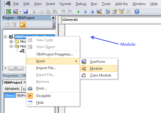
- Press Alt-F11 to open visual basic editor
- Press with left mouse button on Module on the Insert menu
- Copy and paste the above user defined function
- Exit visual basic editor
Fuzzy lookup category
More than 1300 Excel formulasExcel categories
19 Responses to “Fuzzy VLOOKUP”
Leave a Reply
How to comment
How to add a formula to your comment
<code>Insert your formula here.</code>
Convert less than and larger than signs
Use html character entities instead of less than and larger than signs.
< becomes < and > becomes >
How to add VBA code to your comment
[vb 1="vbnet" language=","]
Put your VBA code here.
[/vb]
How to add a picture to your comment:
Upload picture to postimage.org or imgur
Paste image link to your comment.
[...] Excel udf: Fuzzy lookups Filed in Excel, Search/Lookup, User defined functions (udf), vba, Vlookup on Apr.04, 2011. Email This article to a Friend In this post I will describe a basic user defined function with better search functionality than the array formula in this post: Fuzzy vlookup. [...]
I absolutely love the way you think!
I am trying to alter this code to search a closed workbook. My first effort failed so I concluded it can not do this. Is this correct?
What I tried:
1. I duplicated your example. (I could have opened your file but I wanted to learn the code by doing it the long way.)
2. I replaced the range name "List2" with the range name of my search range. [Inven22.xlsm]Catalog!Catalog[Item Description] This file has 2,300 records of which the cells lengths do not exceed 255 char's.
Thanks in advance
I've added your site to my favorites and I'm passing you on to my friends.
Allan,
Thank you for commenting!
I replaced "List2" with a cell reference to a cell range in a closed workbook. Entered the new formula as an array formula. And it worked!
I think you forgot to create an array formula.
1. Replace all instances of List2 with the new cell reference. I used notepad and search/replace.
2. Press and hold Ctrl + Shift
3. Press Enter
4. Release all keys.
Follow up:
I think you may need the code.
Note that the "[" & "]" are removed after selecting Ctrl Shift Enter
Allan,
That is weird.
My cell reference looks like this, after creating the array formula.
[Inven22.xlsm]!Catalog[Item Description]
What error do you get? #NAME?
Thanks for your reply.
I do not get an error, only a blank field.
Allan
Oscar,
I spent hours into the night on this issue and could not figure it out. After posting my last response this morning, it dawned on me that it could be related to the formatting of the file I'm searching.
With that, I created a new test inventory file from scratch and only copied 15 records from the original file and it worked!!
But....I then copied all the records and it failed. It did not return an error but another blank field.
I now have a new direction to focus more troubleshooting towards and will report back.
This is very important for me to achieve. Any thoughts of any kind would be appreciated.
Allan
Oscar,
At this point, I am at a total loss at my findings.
Here are the steps I took:
First - I left a formula unchanged in cell C2 searching the range of the original inventory file that returns a blank.
Second - In Cell C3, I altered formula to search the new file with all the 2303 records.
Responses when searching the new test file:
1. I changed the formula range to search all but 20 records - it worked!
2. Added the full range back to the formula - failed.
3. Cut the range in half - failed.
4. Cut the range another half - failed.
5. Cut the range down to 100 records - success!
6. Increased the range by 500 records - success!
7. Went back to the FULL range - SUCCESS!! ?????
Here is the more interesting issue. After step 7, the formula in C2 went from blank to displaying a correct response!!
What is going on?!?!? I can not trust this formula if it is going to respond this way.
Allan
Alan,
I think I understand. You don´t see the error because the IFERROR function removes errors. That is why you sometimes get a blank cell.
I think it has to do when you enter an array formula. If you don´t enter it correctly you get a regular formula and the IFERROR function removes the error and the output becomes blank.
I should have mentioned this from the beginning, sorry. I am happy you got it working!
I apologize for the non-stop msg's - but it helps me think about other possibilities by trying to explain it to you..
The blank cell makes sense now. I briefly thought about that yesterday while drilling your formula but got side tracked and forgot.
However, I believe the issue still stands. Why would the results return an error on some occasions but not others just by changing the range? More so, changing it from one range that returned an error to another yielding an error ...... then changing it back to the original range which DOES NOT return an error. ???
More importantly, why did the returned error in C2 change to a correct return after I was working on the ranges in C3? Keep in mind, I never edited C2 when this occurred. It did it on its own.
------------------------------------------------------------------
On a second note, I applied the formula to the Item # column and the return is not anywhere close to the expectation.
For ex:
search for item# 1103252507 (which doesn't exist)
- I expect a return of 1103252505 (which does exist, record# 85)
But the return is 3205021007 (record# 275) - way off base.
Can you offer your thoughts on both these issues?
Allan
Allan,
Why would the results return an error on some occasions but not others just by changing the range? More so, changing it from one range that returned an error to another yielding an error ...... then changing it back to the original range which DOES NOT return an error. ???
I have another theory. The array formula is slow. It takes time to calculate. Perhaps when you think it returned a blank cell, it is still calculating. Remove the IFERROR function and try it again. This time it won´t return blank cells.
Good thought; i'll give that a try and get back to you.
I also thought time would be an issue so I made sure to give it plenty - several minutes. I even manually calculated after giving it time and then adding more time. However, I have not tried removing the IfError function.
I hear you saying to drill the whole function down to its primary parts prior to adding the "perks" to it in order to locate the source of the issue. That will take me some time but it'll be fun.
Wish me luck.
Thanks
AC
Oscar,
I've been assuming this function is able to search a closed workbook. Is that correct?
AC
Allan,
I've been assuming this function is able to search a closed workbook. Is that correct?
Yes, I got it working with a closed workbook.
This could be considered harassment at this point.
Current method:
We use an estimating program that searches an external inventory file (managed by the corporate office) by indexing the item # to get the pricing. The current code accounts for missing items by returning the closest match via the "-1" option. As you know, the file must be sorted if we use the "-1" option of the function. In many cases, this returns an item that is not anywhere close to the item being sought.
Goal:
The salesmen have asked me to figure out a way to make this more accurate. Your code - if it can search a closed external file - is exactly what I am looking for because the Fuzzy-vlookup can not read a closed file. Therefor, once my current code locates the closest matched item #, your code could return an item by searching a range of the descriptions based on the item #'s row address.
With that, your array formula provides more than one close item of which I could derive the correct item.
1. If your array formula cannot search a closed file, can it be modified to do so?
2. What prevents it this; the array portion of the code?
3. Should I write code that temporally returns a range above and below the found item# to the estimate sheet to which I could then apply your array formula?
Example items being sought: Actual items in the closed file:
2"x1½"x1½" CI Red. Tee 2"x1½"x1" CI Red. Tee
2½"x2" CI 90° Elbow 2½"x1" CI 90° Reducing Elbow
2½"X1½" Rbrs Red Adapt Fxm 2½"x1½" Rbrs Red Adapt Fxm
2½"X1½" Black CI Flg Con Red 2½"x2" Black CI Flanged Concentric Reducer
2½"x2½"x¾" CI Red. Tee 2½"x2½"x½" CI Red. Tee
Item 3's for above Descr:
1103201515 1103201510
1101002520 1101002510
40CWH0CG25 FHADBRFMEC
As you can see, the corporate office has not developed a schema for the item #'s that can be universally applied. But....the majority of them are. This is the core issue but until they put this on top of their priorities list, I have to deal with it.
Any thoughts or guidance would be greatly appreciated.
Allan
Oscar,
I can't thank you enough for helping me with my issues. Your formula is perfect for my needs and I'm determined to get it working.
I did as you suggested and removed the IfError. It returns a #N/A. With that, I played around with the cell data types, blanks, quantity of records etc. and could only get it to work when there aren't that many records. But even this is hit and miss. Does this help you point me in another direction?
Your suggestion that it may be a time issue did not pan out. The speed is actually pretty nice considering what you've got it doing. When it is working, it's at times when there are not many records. The most I've been able to read and get no errors was the time I mentioned to you already. But as soon as I closed the file, they immediately went error.
I get the same response when the records are on another sheet or workbook. It boils down to the number of records. I believe this is the key to resolving the matter.
I even thought it could be memory related. But I've got 4GB with 8 virtual and Dual Processors so I doubt that could be it. WIN 7 handles it's cache better than the other OS's so I discount that.
Can you help me break this down into smaller segments that will help me narrow it down? Or do you have any tricks that will help determine why the quantity of records is giving it trouble.
Again, thank you for your valuable time.
Any thoughts you can offer are greatly needed and appreciated.
Allan
Allan,
Upload your workbook and I´ll see if I can narrow it down.
Is is possible if the script find different values? I mean multiple occurences if find multiple matches?
Thanks
Rizkyu
[…] https://www.get-digital-help.com/excel-udf-fuzzy-lookups/ […]