Working with overlapping date ranges

This article demonstrates formulas that calculate the number of overlapping ranges for all ranges, finds the most overlapped range and the least overlapped range.
Today's blog post is about date ranges, the techniques demonstrated here can also be applied to Excel time values or other numerical ranges.
The MMULT function is a great excel function, it allows you to do really amazing calculations with date ranges. Yes, I have said that before.
What's on this webpage
- Calculate the number of overlapping date ranges
- Calculate the number of overlapped ranges for all ranges in one formula?
- Find most overlapped date range
- Least overlapped date range
- Most overlapped date
- Least overlapped date
- Get Excel file
- Count overlapping days across multiple date ranges
- Count overlapping days in multiple date ranges
- Count overlapping days in multiple date ranges, part 2
- Find empty dates in a set of date ranges
- List dates outside specified date ranges
1. Calculate the number of overlapping date ranges

For simplicity, in this example, there are only 4 date ranges in column B and C and you can see their length in the chart to the right.
Let's begin with a simple formula, it will be helpful for you if you understand this one. It calculates the number of date ranges that overlaps the first date range:
It returns 3 overlapping date ranges, which is correct. Range 2, 3 and 4 overlap range 1.
Read this post if you want to know more about this formula:
Find overlapping date ranges.
2. Calculate the number of overlapped ranges for all ranges in one formula?
How do we calculate the number of overlapped ranges for all ranges in one formula?
This array formula returns an array: {3;2;2;1} which corresponds to the position of each date range in row 3, 4, 5, and 6.
The first date range has 3 overlapping ranges, described above. The second has 2, range 1 and 3 overlaps range 2.
The third has 2 overlapping ranges, range 1 and 2. The fourth range has 1 overlapping date range, range 1.
Explaining formula in cell I9
Step 1 - Transpose array
The TRANSPOSE function converts a vertical range to a horizontal range, or vice versa.
TRANSPOSE(D3:D6)
becomes
TRANSPOSE({42020; 42009; 42013; 42024})
and returns {42020, 42009, 42013, 42024}
Step 2 - Logical test 1
The less than character and the equal character combined means less than or equal to.
C3:C6<=TRANSPOSE(D3:D6)
becomes
C3:C6<={42020, 42009, 42013, 42024}
becomes
{42007; 42006; 42008; 42016}<={42020, 42009, 42013, 42024}
and returns
{TRUE, TRUE, TRUE, TRUE; TRUE, TRUE, TRUE, TRUE; TRUE, TRUE, TRUE, TRUE; TRUE, FALSE, FALSE, TRUE}
Step 3 - Logical test 2
D3:D6>=TRANSPOSE(C3:C6)
becomes
{42020;42009;42013;42024}>={42007,42006,42008,42016}
and returns
{TRUE, TRUE, TRUE, TRUE; TRUE, TRUE, TRUE, FALSE; TRUE, TRUE, TRUE, FALSE; TRUE, TRUE, TRUE, TRUE}.
Step 4 - Multiply arrays
When we multiply arrays we need to make sure the size of one array matches the other array. Multiplying boolean values is the same as applying AND logic. The result is the numerical equivalent TRUE = 1 and FALSE = 0 (zero).
TRUE * TRUE = 1, TRUE * FALSE = 0 (zero) and, FALSE * FALSE = 0 (zero).
(C3:C6<=TRANSPOSE(D3:D6))*(D3:D6>=TRANSPOSE(C3:C6))
becomes
{TRUE, TRUE, TRUE, TRUE; TRUE, TRUE, TRUE, TRUE; TRUE, TRUE, TRUE, TRUE; TRUE, FALSE, FALSE, TRUE}*{TRUE, TRUE, TRUE, TRUE; TRUE, TRUE, TRUE, FALSE; TRUE, TRUE, TRUE, FALSE; TRUE, TRUE, TRUE, TRUE}
and returns {1, 1, 1, 1; 1, 1, 1, 0; 1, 1, 1, 0; 1, 0, 0, 1}.
Step 5 - Create an array containing 1
Exponentiation is a mathematical operation, use the ^ character or the POWER function to calculate the result of exponentiation.
When a number is raised to the power of 0 (zero) the result is always 1.
C3:C6^0
becomes
{42007;42006;42008;42016}^0
and returns {1;1;1;1}.
Step 6 - Evaluate MMULT function
The MMULT function calculates the matrix product of two arrays, an array as the same number of rows as array1 and columns as array2.
MMULT(array1, array2)
MMULT((C3:C6<=TRANSPOSE(D3:D6))*(D3:D6>=TRANSPOSE(C3:C6)),C3:C6^0)
becomes
MMULT({1, 1, 1, 1; 1, 1, 1, 0; 1, 1, 1, 0; 1, 0, 0, 1}, {1;1;1;1})
and returns {4; 3; 3; 2}.
Step 7 - Subtract with 1
The MMULT function calculates all overlapping ranges even the range itself. We need to subtract with 1 to get the correct result.
MMULT((C3:C6<=TRANSPOSE(D3:D6))*(D3:D6>=TRANSPOSE(C3:C6)),C3:C6^0)-1
becomes
{4; 3; 3; 2}-1
and returns {3; 2; 2; 1}.
2.1 Use a drop-down list to select a date range to see overlapping date ranges

In the animated picture above the drop-down list in cell D7 allows you to select a date range, cell D8 tells you how many overlapping date ranges the selected date range has.
I applied conditional formatting to easily spot the selected date range.
Array formula in cell D8:
3. Find most overlapped date range
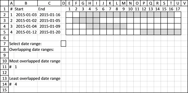
Using this technique we can now construct a formula that finds the most overlapped date range, array formula in cell B11:
Want to know more about the excel functions used in the formulas above?
SUMPRODUCT, MMULT, INDEX, MATCH
4. Least overlapped date range
Array formula in cell B14:
5. Most overlapped date

Array formula in cell C18:
6. Least overlapped date

Array formula in cell C21:
Interested in learning more about excel, join my Advanced excel course.
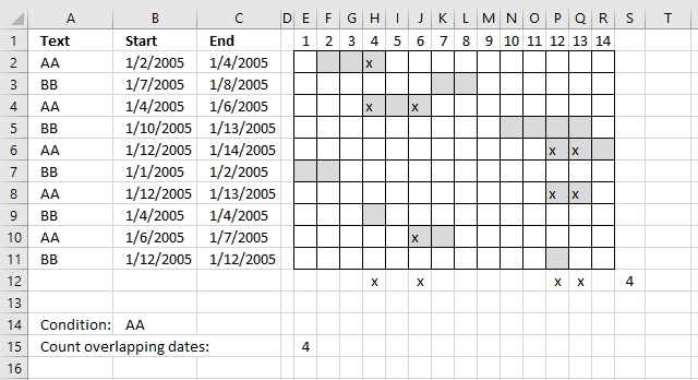
8. Count overlapping days across multiple date ranges
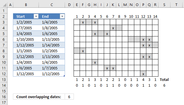
This post demonstrates a formula in cell D16 that counts overlapping dates across multiple date ranges. The date ranges are specified in the Excel Table column Start and End (cell range B3:B12 and C3:C12), see image above.
To the right is a part of a calendar with date 1 to 14, the gray cells are days based on the corresponding date range. The x's are dates that overlap another date.
Row 13 contains the sum of these gray days column-wise, row 14 contains 1 or 0 (zero) indicating if the date contains a date range that overlaps another date range. Cell S14 contains a total of these overlapping dates. This is only demonstrated to show that the calculation is in fact correct.
NC asks:
Thanks a tonne, Oscar. It took me about 8 hours to work through this formula piece by piece, play with it, and come to grips with its basics. Your example was clear and very useful, and this has allowed me to do big, very useful data analysis for the company that employs me. It applies to thousands of people. You're an unsung hero.
Actually just realized that I really need what you said you'd "save for a future post" (actually total number of overlapping dates). I guess I'll try to figure that out. Still... couldn't have gotten this close without you.
Answer:
Thanks NC, here comes that "future" post. Array formula in cell D16:
To enter an array formula you copy above formula and paste to a cell. Press and hold CTRL and Shift simultaneoulsy, then press Enter once. Release all keys.
The formula is now surrounded with curly brackets, don't enter these characters yourself, they appear automatically. {=formula}
Explaining formula in cell D16
Step 1 - Create array
The power of sign ^ converts all dates in Table column Start to 1, you can also use the POWER function, however, to keep the formula as small as possible I use ^.
TRANSPOSE(Table1[Start]^0)
becomes
TRANSPOSE({38354; 38359; 38356; 38362; 38364; 38353; 38364; 38356; 38358; 38364}^0)
becomes
TRANSPOSE({1; 1; 1; 1; 1; 1; 1; 1; 1; 1})
The TRANSPOSE function converts a vertical range to a horizontal range, or vice versa.
TRANSPOSE({1; 1; 1; 1; 1; 1; 1; 1; 1; 1})
returns
{1, 1, 1, 1, 1, 1, 1, 1, 1, 1}
This array is needed in the first argument in the MMULT function.
Step 2 - Create an array containing dates
This step calculates the dates needed based on the earliest and latest date in columns Table1[Start] and Table1[End].
(TRANSPOSE(MIN(Table1[Start])+ROW(B1:INDEX($B:$B,MAX(Table1[End])-MIN(Table1[Start])+1))-1)
becomes
(TRANSPOSE(MIN({38354; 38359; 38356; 38362; 38364; 38353; 38364; 38356; 38358; 38364})+ROW(B1:INDEX($B:$B,MAX(Table1[End])-MIN(Table1[Start])+1))-1)
becomes
(TRANSPOSE(38353+ROW(B1:INDEX($B:$B,MAX(Table1[End])-MIN(Table1[Start])+1))-1)
becomes
(TRANSPOSE(38353+ROW(B1:INDEX($B:$B,MAX({38356; 38360; 38358; 38365; 38366; 38354; 38365; 38356; 38359; 38364})-MIN(Table1[Start])+1))-1)
becomes
(TRANSPOSE(38353+ROW(B1:INDEX($B:$B,38366-MIN(Table1[Start])+1))-1)
becomes
(TRANSPOSE(38353+ROW(B1:INDEX($B:$B,38366-38353+1)))-1)
becomes
(TRANSPOSE(38353+ROW(B1:INDEX($B:$B,13+1)))-1)
becomes
(TRANSPOSE(38353+ROW(B1:INDEX($B:$B,14)))-1)
becomes
(TRANSPOSE(38353+ROW(B1:$B14))-1)
becomes
(TRANSPOSE(38353+{1; 2; 3; 4; 5; 6; 7; 8; 9; 10; 11; 12; 13; 14})-1)
becomes
(TRANSPOSE({38354; 38355; 38356; 38357; 38358; 38359; 38360; 38361; 38362; 38363; 38364; 38365; 38366; 38367})-1)
becomes
(TRANSPOSE(38353+{0; 1; 2; 3; 4; 5; 6; 7; 8; 9; 10; 11; 12; 13})
and returns
{38353, 38354, 38355, 38356, 38357, 38358, 38359, 38360, 38361, 38362, 38363, 38364, 38365, 38366}
Step 3 - Check which dates are later or equal to dates in Table column Start
(TRANSPOSE(MIN(Table1[Start])+ROW(B1:INDEX($B:$B,MAX(Table1[End])-MIN(Table1[Start])+1))-1)>=Table1[Start]
becomes
{38353, 38354, 38355, 38356, 38357, 38358, 38359, 38360, 38361, 38362, 38363, 38364, 38365, 38366}>=Table1[Start]
becomes
{38353, 38354, 38355, 38356, 38357, 38358, 38359, 38360, 38361, 38362, 38363, 38364, 38365, 38366}>={38354; 38359; 38356; 38362; 38364; 38353; 38364; 38356; 38358; 38364}
and returns this array:
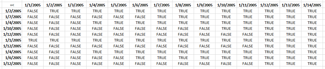
I have added the dates horizontally and vertically to make this picture more easy to understand.
Step 4 - Repeat step 2 and 3 with Table column End
((TRANSPOSE(MIN(Table1[Start])+ROW(B1:INDEX($B:$B,MAX(Table1[End])-MIN(Table1[Start])+1))-1))<=Table1[End]))>1)
returns this array:
Step 5 - Multiply arrays
(TRANSPOSE(MIN(Table1[Start])+ROW(B1:INDEX($B:$B, MAX(Table1[End])-MIN(Table1[Start])+1))-1)>=Table1[Start])*((TRANSPOSE(MIN(Table1[Start])+ROW(B1:INDEX($B:$B, MAX(Table1[End])-MIN(Table1[Start])+1))-1))<=Table1[End])
returns this array:
Step 6 - Sum values column-wise
MMULT(TRANSPOSE(Table1[Start]^0), (TRANSPOSE(MIN(Table1[Start])+ROW(B1:INDEX($B:$B, MAX(Table1[End])-MIN(Table1[Start])+1))-1)>=Table1[Start])*((TRANSPOSE(MIN(Table1[Start])+ROW(B1:INDEX($B:$B, MAX(Table1[End])-MIN(Table1[Start])+1))-1))<=Table1[End]))
returns
{1, 2, 1, 3, 1, 2, 2, 1, 0, 1, 1, 4, 3, 1}
Step 7 - Check if value in array is larger than 1
MMULT(TRANSPOSE(Table1[Start]^0), (TRANSPOSE(MIN(Table1[Start])+ROW(B1:INDEX($B:$B, MAX(Table1[End])-MIN(Table1[Start])+1))-1)>=Table1[Start])*((TRANSPOSE(MIN(Table1[Start])+ROW(B1:INDEX($B:$B, MAX(Table1[End])-MIN(Table1[Start])+1))-1))<=Table1[End]))>1
becomes
{1, 2, 1, 3, 1, 2, 2, 1, 0, 1, 1, 4, 3, 1}>1
and returns
{FALSE, TRUE, FALSE, TRUE, FALSE, TRUE, TRUE, FALSE, FALSE, FALSE, FALSE, TRUE, TRUE, FALSE}
Step 8 - Convert boolean values to their numerical equivalents
(MMULT(TRANSPOSE(Table1[Start]^0), (TRANSPOSE(MIN(Table1[Start])+ROW(B1:INDEX($B:$B, MAX(Table1[End])-MIN(Table1[Start])+1))-1)>=Table1[Start])*((TRANSPOSE(MIN(Table1[Start])+ROW(B1:INDEX($B:$B, MAX(Table1[End])-MIN(Table1[Start])+1))-1))<=Table1[End]))>1)*1
becomes
{FALSE, TRUE, FALSE, TRUE, FALSE, TRUE, TRUE, FALSE, FALSE, FALSE, FALSE, TRUE, TRUE, FALSE}*1
and returns
{0, 1, 0, 1, 0, 1, 1, 0, 0, 0, 0, 1, 1, 0}
Step 9 - Sum overlapping dates
SUM((MMULT(TRANSPOSE(Table1[Start]^0), (TRANSPOSE(MIN(Table1[Start])+ROW(B1:INDEX($B:$B, MAX(Table1[End])-MIN(Table1[Start])+1))-1)>=Table1[Start])*((TRANSPOSE(MIN(Table1[Start])+ROW(B1:INDEX($B:$B, MAX(Table1[End])-MIN(Table1[Start])+1))-1))<=Table1[End]))>1)*1)
becomes
SUM({0, 1, 0, 1, 0, 1, 1, 0, 0, 0, 0, 1, 1, 0})
and returns 6 in cell D16.
Count overlapping days across multiple date ranges with condition
This formula takes into account the condition specified in cell E15 as well, the formula counts overlapping dates based on date ranges that has a cell in column A which is equal to the condition in cell B14.
Formula in cell E15:
The only difference with the formula above is this part:
($A$2:$A$11=$B$14)
It is a logical expression that returns an array containing TRUE or FALSE if equal to value in cell B14.
9. Count overlapping days in multiple date ranges
The MEDIAN function lets you count overlapping dates between two date ranges. If you have more than two date ranges you need to use a more complicated array formula.
What's on this section
- Count overlapping days for all date ranges
- Count all overlapping days
9.1. Count overlapping days for all date ranges

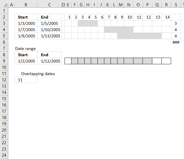
I have three date ranges (B3:C5) in this example and I want to count the number of days that overlap another date range (B9:C9).
This array formula counts overlapping days for each date range in cell range B3:C5 compared to the date range in cell range B9:C9.
Array formula in cell S3:S5:
Excel 365 formula in cell R2:
The Excel 365 formula above is a dynamic array formula and works only in Excel 365.
Both formulas above return this array: {3; 4; 1}, the numbers correspond to the date ranges in rows 2,3, and 4.
Date range 2005-01-03/2005-01-05 (A2:B2) has 3 overlapping dates compared to 2005-01-02/2005-01-12 (A8:B8).
Date range 2005-01-07/2005-01-10 (A3:B3) has 4 overlapping dates compared to 2005-01-02/2005-01-12 (A8:B8).
Date range 2005-01-12/2005-01-13 (A3:B3) has 1 overlapping date compared to 2005-01-02/2005-01-12 (A8:B8).
Explaining formula in cell S3:S5
Step 1 - Count days in date range
$C$9-$B$9+1
becomes
38364-38354+1
and returns 11.
Step 2 - Create a cell reference
The INDEX function is also able to create a cell reference.
INDEX($B:$B, $C$9-$B$9+1)
becomes
INDEX($B:$B, 11)
and returns A11.
Step 3 - Concatenate cell references
A1:INDEX($A:$A, $C$9-$B$9+1)
returns A1:A11.
Step 4 - Calculate row numbers based on cell reference
The ROW function returns a row number from a cell reference. It returns multiple row numbers if the cell reference points to a cell range.
ROW(A1:INDEX($A:$A, $C$9-$B$9+1))
becomes
ROW(A1:A11)-1
and returns {1; 2; 3; 4; 5; 6; 7; 8; 9; 10; 11}
Step 5 - Subtract with 1
ROW(A1:INDEX($A:$A, $C$9-$B$9+1))-1
becomes
{1; 2; 3; 4; 5; 6; 7; 8; 9; 10; 11} - 1
and returns
{0; 1; 2; 3; 4; 5; 6; 7; 8; 9; 10}
Step 6 - Add array to start date
$B$9+ROW(A1:INDEX($A:$A, $C$9-$B$9+1))-1
becomes
38354+{0; 1; ... ; 10}
and returns {38354; ... ; 38364}
Step 7 - Convert vertical array to a horizontal array
The TRANSPOSE function allows you to convert a vertical range to a horizontal range, or vice versa.
TRANSPOSE(array)
TRANSPOSE($B$9+ROW(A1:INDEX($A:$A, $C$9-$B$9+1))-1)
returns {38354, 38355, ... , 38364}
Step 8 - Test which dates are larger or equal to start dates
TRANSPOSE($B$9+ROW(A1:INDEX($A:$A,$C$9-$B$9+1))-1)>=$B$3:$B$5
returns {FALSE, TRUE, ... , TRUE}
Step 9 - Test which dates are smaller or equal to end dates
TRANSPOSE($B$9+ROW(A1:INDEX($A:$A,$C$9-$B$9+1))-1)<=C3:C5
returns {TRUE, TRUE, ... , TRUE}
Step 10 - Multiply arrays
This step identifies dates inside a date range, both arrays must return TRUE to return TRUE which is the same as AND-logic.
(TRANSPOSE($B$9+ROW(A1:INDEX($A:$A,$C$9-$B$9+1))-1)>=$B$3:$B$5)*(TRANSPOSE($B$9+ROW(A1:INDEX($A:$A,$C$9-$B$9+1))-1)<=C3:C5)
returns {0, 1, ... , 1}.
Note that 1 is equal to the boolean value TRUE and 0 (zero) is FALSE.
Step 11 - Create an array of numbers all equal to 1
Exponentiation is a mathematical operation, use the ^ character or the POWER function to calculate the result of exponentiation.
When a number is raised to the power of 0 (zero) the result is always 1. This makes it easy to create an array of numbers all equal to 1.
ROW(A1:INDEX($A:$A,$C$9-$B$9+1))^0
returns {1; ... ; 1}
Step 12 - Evaluate MMULT function
The MMULT function calculates the matrix product of two arrays, an array as the same number of rows as array1 and columns as array2.
MMULT((TRANSPOSE($B$9+ROW(A1:INDEX($A:$A,$C$9-$B$9+1))-1)>=$B$3:$B$5)*(TRANSPOSE($B$9+ROW(A1:INDEX($A:$A,$C$9-$B$9+1))-1)<=C3:C5),ROW(A1:INDEX($A:$A,$C$9-$B$9+1))^0)
returns {3;4;4}.
9.2. Count all overlapping days

To count all overlapping days, array formula in cell B12:
Functions in array formulas: MMULT, ROW, INDEX
Overlapping date ranges in cell range A2:B4
Keep in mind that if you have overlapping date ranges in A2:B4, overlapping dates will be counted twice or more.
In this example, date 9 and 10 are overlapped by 2005-01-07/2005-01-10 and 2005-01-09/2005-01-13. They are counted twice, see values above in cell range S4:S5.
The value in cell A11 is wrong because of this, only 9 dates are overlapped. There is a formula for this scenario also but I'll save it for a future post.
10. Count overlapping days in multiple date ranges, part 2

In the previous post I explained how to count overlapping dates comparing a single date range against multiple date ranges. In this section, I will demonstrate how to count overlapping dates across multiple date ranges.
The date ranges are in columns A and B. The calendar to the right is there so that you can easily verify that the formula is correct.
What's on this webpage
- Count the number of overlapping date ranges for each date
- Count dates overlapped by two or more date ranges
- Get Excel file
10.1. Count the number of overlapping date ranges for each date
The first formula returns an array that counts the number of overlapping date ranges for each date. It is shown in cell range D12:Q12.
The formula returns this array: {1, 2, 1, 3, 1, 2, 2, 1, 0, 1, 1, 4, 3, 1}
Date 2005-01-01 is overlapped once by date range 2005-01-01/2005-01-02. So the first value in the array is 1.
Date 2005-01-02 is overlapped twice by date range 2005-01-01/2005-01-02 and 2005-01-02/2005-01-04. The second value in the array is 2.
...
Date 2005-01-09 is not overlapped at all so the ninth value in the array is 0 (zero).
And so on.., you can verify these numbers against the calendar above.
10.2. Count dates overlapped by two or more date ranges
The second array formula returns an array that indicates if a date is overlapped by two or more date ranges. It is entered in cell range E14:R14.
This formula returns {0, 1, 0, 1, 0, 1, 1, 0, 0, 0, 0, 1, 1, 0}
If we sum this array we get the total number of overlapped dates. That value is shown cell D15 and R13.
10.2.1 Explaining formula in cell range D13:Q13
Step 1 - Find latest date in end dates
The MAX function returns the largest number from a cell range or array.
MAX($C$3:$C$12)
becomes
MAX({38356; 38360; 38358; 38365; 38366; 38354; 38365; 38356; 38359; 38364})
and returns 38366. Note that these numbers are actually Excel dates, numbers formatted as dates. 38366 is 1/14/2005.
Step 2 - Find earliest date in start dates
The MIN function returns the largest number from a cell range or array.
MIN($B$3:$B$12)
becomes
MIN({38354; 38359; 38356; 38362; 38364; 38353; 38364; 38356; 38358; 38364})
and returns 38353.
Step 3 - Subtract dates
MAX($C$3:$C$12)-MIN($B$3:$B$12)+1))+1
becomes
38366 - 38353 +1 equals 14.
Step 4 - Create a cell reference
The INDEX function is also able to create a cell reference.
INDEX($A:$A, MAX($C$3:$C$12)-MIN($B$3:$B$12)+1)
becomes
INDEX($A:$A, 14)
and returns cell reference A14.
Step 5- Concatenate cell references
You need to use the ampersand character & to concatenate strings, however, not necessary in this rare case.
A1:INDEX($A:$A, MAX($C$3:$C$12)-MIN($B$3:$B$12)+1)
returns cell reference A1:A14.
Step 6 - Calculate row numbers based on a cell reference
The ROW function returns a row number from a cell reference. It returns multiple row numbers if the cell reference points to a cell range.
ROW(A1:INDEX($A:$A, MAX($B$2:$B$11)-MIN($A$2:$A$11)+1))
becomes
ROW( A1:A14)
and returns {1; 2; 3; 4; 5; 6; 7; 8; 9; 10; 11; 12; 13; 14}.
Step 5 - Subtract array with 1
ROW(A1:INDEX($A:$A, MAX($B$2:$B$11)-MIN($A$2:$A$11)+1))-1
becomes
{1; 2; 3; 4; 5; 6; 7; 8; 9; 10; 11; 12; 13; 14}-1
and returns
{0; 1; 2; 3; 4; 5; 6; 7; 8; 9; 10; 11; 12; 13;}
Step 6 - Add array to earliest start date
MIN($B$3:$B$12)+ROW(A1:INDEX($A:$A, MAX($C$3:$C$12)-MIN($B$3:$B$12)+1))-1
becomes
38353+ROW(A1:INDEX($A:$A, MAX($C$3:$C$12)-MIN($B$3:$B$12)+1))-1
becomes
38353 + {0; 1; 2; 3; 4; 5; 6; 7; 8; 9; 10; 11; 12; 13;}
and returns
{38353; 38354; 38355; 38356; 38357; 38358; 38359; 38360; 38361; 38362; 38363; 38364; 38365; 38366}
Step 7 - Convert vertical array to a horizontal array
The TRANSPOSE function allows you to convert a vertical range to a horizontal range, or vice versa.
TRANSPOSE(array)
TRANSPOSE(MIN($B$3:$B$12)+ROW(A1:INDEX($A:$A, MAX($C$3:$C$12)-MIN($B$3:$B$12)+1))-1)
becomes
TRANSPOSE({38353; 38354; 38355; 38356; 38357; 38358; 38359; 38360; 38361; 38362; 38363; 38364; 38365; 38366})
and returns
{38353, 38354, 38355, 38356, 38357, 38358, 38359, 38360, 38361, 38362, 38363, 38364, 38365, 38366}
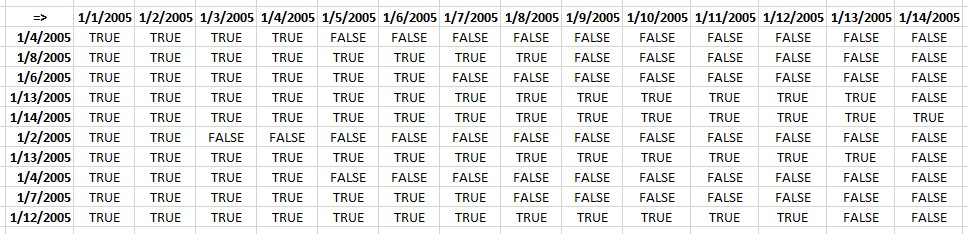
Step 8 - Test which dates are larger or equal to start dates
TRANSPOSE(MIN($B$3:$B$12)+ROW(A1:INDEX($A:$A, MAX($C$3:$C$12)-MIN($B$3:$B$12)+1))-1)>=$B$3:$B$12
becomes
{38353, 38354, 38355, 38356, 38357, 38358, 38359, 38360, 38361, 38362, 38363, 38364, 38365, 38366}>={38354; 38359; 38356; 38362; 38364; 38353; 38364; 38356; 38358; 38364}
and returns
{FALSE, TRUE, TRUE, TRUE, TRUE, TRUE, TRUE, TRUE, TRUE, TRUE, TRUE, TRUE, TRUE, TRUE;FALSE, FALSE, FALSE, FALSE, FALSE, FALSE, TRUE, TRUE, TRUE, TRUE, TRUE, TRUE, TRUE, TRUE;FALSE, FALSE, FALSE, TRUE, TRUE, TRUE, TRUE, TRUE, TRUE, TRUE, TRUE, TRUE, TRUE, TRUE;FALSE, FALSE, FALSE, FALSE, FALSE, FALSE, FALSE, FALSE, FALSE, TRUE, TRUE, TRUE, TRUE, TRUE;FALSE, FALSE, FALSE, FALSE, FALSE, FALSE, FALSE, FALSE, FALSE, FALSE, FALSE, TRUE, TRUE, TRUE;TRUE, TRUE, TRUE, TRUE, TRUE, TRUE, TRUE, TRUE, TRUE, TRUE, TRUE, TRUE, TRUE, TRUE;FALSE, FALSE, FALSE, FALSE, FALSE, FALSE, FALSE, FALSE, FALSE, FALSE, FALSE, TRUE, TRUE, TRUE;FALSE, FALSE, FALSE, TRUE, TRUE, TRUE, TRUE, TRUE, TRUE, TRUE, TRUE, TRUE, TRUE, TRUE;FALSE, FALSE, FALSE, FALSE, FALSE, TRUE, TRUE, TRUE, TRUE, TRUE, TRUE, TRUE, TRUE, TRUE;FALSE, FALSE, FALSE, FALSE, FALSE, FALSE, FALSE, FALSE, FALSE, FALSE, FALSE, TRUE, TRUE, TRUE}
Step 9 - Test which dates are smaller or equal to end dates
TRANSPOSE(MIN($B$3:$B$12)+ROW(A1:INDEX($A:$A, MAX($C$3:$C$12)-MIN($B$3:$B$12)+1))-1))<=$C$3:$C$12
returns
{TRUE, TRUE, TRUE, TRUE, FALSE, FALSE, FALSE, FALSE, FALSE, FALSE, FALSE, FALSE, FALSE, FALSE;TRUE, TRUE, TRUE, TRUE, TRUE, TRUE, TRUE, TRUE, FALSE, FALSE, FALSE, FALSE, FALSE, FALSE;TRUE, TRUE, TRUE, TRUE, TRUE, TRUE, FALSE, FALSE, FALSE, FALSE, FALSE, FALSE, FALSE, FALSE;TRUE, TRUE, TRUE, TRUE, TRUE, TRUE, TRUE, TRUE, TRUE, TRUE, TRUE, TRUE, TRUE, FALSE;TRUE, TRUE, TRUE, TRUE, TRUE, TRUE, TRUE, TRUE, TRUE, TRUE, TRUE, TRUE, TRUE, TRUE;TRUE, TRUE, FALSE, FALSE, FALSE, FALSE, FALSE, FALSE, FALSE, FALSE, FALSE, FALSE, FALSE, FALSE;TRUE, TRUE, TRUE, TRUE, TRUE, TRUE, TRUE, TRUE, TRUE, TRUE, TRUE, TRUE, TRUE, FALSE;TRUE, TRUE, TRUE, TRUE, FALSE, FALSE, FALSE, FALSE, FALSE, FALSE, FALSE, FALSE, FALSE, FALSE;TRUE, TRUE, TRUE, TRUE, TRUE, TRUE, TRUE, FALSE, FALSE, FALSE, FALSE, FALSE, FALSE, FALSE;TRUE, TRUE, TRUE, TRUE, TRUE, TRUE, TRUE, TRUE, TRUE, TRUE, TRUE, TRUE, FALSE, FALSE}
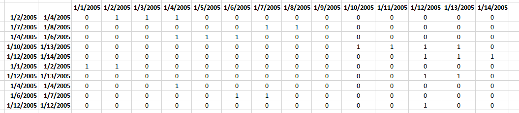
Step 10 - Multiply arrays
(TRANSPOSE(MIN($B$3:$B$12)+ROW(A1:INDEX($A:$A, MAX($C$3:$C$12)-MIN($B$3:$B$12)+1))-1)>=$B$3:$B$12)*((TRANSPOSE(MIN($B$3:$B$12)+ROW(A1:INDEX($A:$A, MAX($C$3:$C$12)-MIN($B$3:$B$12)+1))-1))<=$C$3:$C$12)
returns
{0, 1, 1, 1, 0, 0, 0, 0, 0, 0, 0, 0, 0, 0;0, 0, 0, 0, 0, 0, 1, 1, 0, 0, 0, 0, 0, 0;0, 0, 0, 1, 1, 1, 0, 0, 0, 0, 0, 0, 0, 0;0, 0, 0, 0, 0, 0, 0, 0, 0, 1, 1, 1, 1, 0;0, 0, 0, 0, 0, 0, 0, 0, 0, 0, 0, 1, 1, 1;1, 1, 0, 0, 0, 0, 0, 0, 0, 0, 0, 0, 0, 0;0, 0, 0, 0, 0, 0, 0, 0, 0, 0, 0, 1, 1, 0;0, 0, 0, 1, 0, 0, 0, 0, 0, 0, 0, 0, 0, 0;0, 0, 0, 0, 0, 1, 1, 0, 0, 0, 0, 0, 0, 0;0, 0, 0, 0, 0, 0, 0, 0, 0, 0, 0, 1, 0, 0}
Step 11 - Create an array of numbers all equal to 1
Exponentiation is a mathematical operation, use the ^ character or the POWER function to calculate the result of exponentiation.
TRANSPOSE($B$3:$B$12^0)
becomes
TRANSPOSE({38354; 38359; 38356; 38362; 38364; 38353; 38364; 38356; 38358; 38364}^0)
becomes
TRANSPOSE({1; 1; 1; 1; 1; 1; 1; 1; 1; 1})
and returns {1, 1, 1, 1, 1, 1, 1, 1, 1, 1}.
Step 12 - Evaluate MMULT function
The MMULT function calculates the matrix product of two arrays, an array as the same number of rows as array1 and columns as array2.
MMULT(TRANSPOSE($B$3:$B$12^0), (TRANSPOSE(MIN($B$3:$B$12)+ROW(A1:INDEX($A:$A, MAX($C$3:$C$12)-MIN($B$3:$B$12)+1))-1)>=$B$3:$B$12)*((TRANSPOSE(MIN($B$3:$B$12)+ROW(A1:INDEX($A:$A, MAX($C$3:$C$12)-MIN($B$3:$B$12)+1))-1))<=$C$3:$C$12))
becomes
MMULT({1, 1, 1, 1, 1, 1, 1, 1, 1, 1}, {0, 1, 1, 1, 0, 0, 0, 0, 0, 0, 0, 0, 0, 0;0, 0, 0, 0, 0, 0, 1, 1, 0, 0, 0, 0, 0, 0;0, 0, 0, 1, 1, 1, 0, 0, 0, 0, 0, 0, 0, 0;0, 0, 0, 0, 0, 0, 0, 0, 0, 1, 1, 1, 1, 0;0, 0, 0, 0, 0, 0, 0, 0, 0, 0, 0, 1, 1, 1;1, 1, 0, 0, 0, 0, 0, 0, 0, 0, 0, 0, 0, 0;0, 0, 0, 0, 0, 0, 0, 0, 0, 0, 0, 1, 1, 0;0, 0, 0, 1, 0, 0, 0, 0, 0, 0, 0, 0, 0, 0;0, 0, 0, 0, 0, 1, 1, 0, 0, 0, 0, 0, 0, 0;0, 0, 0, 0, 0, 0, 0, 0, 0, 0, 0, 1, 0, 0})
and returns
{1, 2, 1, 3, 1, 2, 2, 1, 0, 1, 1, 4, 3, 1}
Step 13 - Check if value in array is larger than 1
MMULT(TRANSPOSE($B$3:$B$12^0), (TRANSPOSE(MIN($B$3:$B$12)+ROW(A1:INDEX($A:$A, MAX($C$3:$C$12)-MIN($B$3:$B$12)+1))-1)>=$B$3:$B$12)*((TRANSPOSE(MIN($B$3:$B$12)+ROW(A1:INDEX($A:$A, MAX($C$3:$C$12)-MIN($B$3:$B$12)+1))-1))<=$C$3:$C$12))>1
becomes
{1, 2, 1, 3, 1, 2, 2, 1, 0, 1, 1, 4, 3, 1}>1
and returns
{FALSE, TRUE, FALSE, TRUE, FALSE, TRUE, TRUE, FALSE, FALSE, FALSE, FALSE, TRUE, TRUE, FALSE}
Step 14 - Convert boolean values
(MMULT(TRANSPOSE($B$3:$B$12^0), (TRANSPOSE(MIN($B$3:$B$12)+ROW(A1:INDEX($A:$A, MAX($C$3:$C$12)-MIN($B$3:$B$12)+1))-1)>=$B$3:$B$12)*((TRANSPOSE(MIN($B$3:$B$12)+ROW(A1:INDEX($A:$A, MAX($C$3:$C$12)-MIN($B$3:$B$12)+1))-1))<=$C$3:$C$12))>1)*1
becomes
{FALSE, TRUE, FALSE, TRUE, FALSE, TRUE, TRUE, FALSE, FALSE, FALSE, FALSE, TRUE, TRUE, FALSE}*1
and returns
{0, 1, 0, 1, 0, 1, 1, 0, 0, 0, 0, 1, 1, 0}.
Functions in this post: MMULT, ROW, INDEX
11. Find empty dates in a set of date ranges
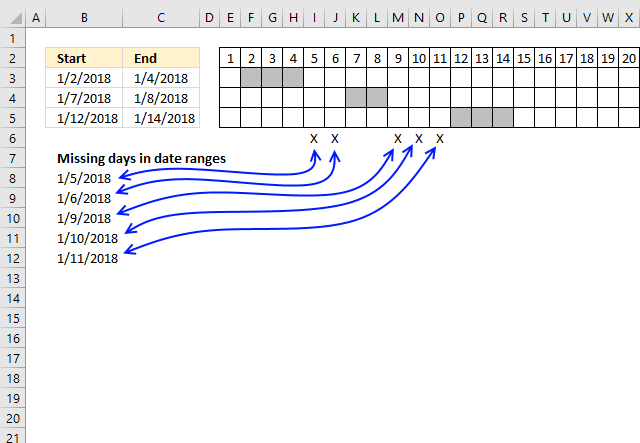
The formula in cell B8, shown above, extracts dates not included in the specified date ranges, in other words, dates that are between date ranges.
I have also built a small calendar using conditional formatting to show exactly where the missing dates are. The formula below works fine with overlapping date ranges.
I will explain the formula in this article and there will also be a file for you to get.
What's on this section
- Find empty dates in a set of date ranges - Excel 365
- Find empty dates in a set of date ranges - earlier versions
11.1. Find empty dates in a set of date ranges - Excel 365

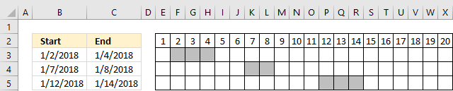
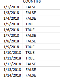
The "X" on row 6 shows which dates are empty or not overlapping the specified date ranges in cells B3:C5. The cells above show which dates each range covers, there are five dates not in any of the date ranges.
Excel 365 dynamic array formula in cell B8:
11.1.1 Explaining formula
Step 1 - Find the latest date
The MAX function calculate the largest number in a cell range.
Function syntax: MAX(number1, [number2], ...)
MAX(B3:C5)
becomes
MAX({43102, 43104; 43107, 43108; 43112, 43114})
and returns 43114. 43114 represents Excel date '1/14/2018'.
Step 2 - Find the earliest date
The MIN function returns the smallest number in a cell range.
Function syntax: MIN(number1, [number2], ...)
MIN(B3:C5)
becomes
MIN({43102, 43104; 43107, 43108; 43112, 43114})
and returns 43102. 43102 represents Excel date '1/2/2018'.
Step 3 - Calculate the difference in days between the earliest date and the latest date
The minus character lets you subtract numbers in an Excel formula.
MAX(B3:C5)-MIN(B3:C5)
becomes
43114-43102 equals 12.
Step 4 - Create a sequence of Excel dates
The SEQUENCE function creates a list of sequential numbers.
Function syntax: SEQUENCE(rows, [columns], [start], [step])
SEQUENCE(MAX(B3:C5)-MIN(B3:C5),,MIN(B3:C5))
becomes
SEQUENCE(12,, 43102)
and returns
{43102; 43103; 43104; 43105; 43106; 43107; 43108; 43109; 43110; 43111; 43112; 43113}.
Step 5 - Check if dates in sequence are larger or equal to the start dates
The less than and equal signs are logical operators that let you compare value to value, in this ,case if a number is smaller than or equal to another number.
B3:B5,"<="&SEQUENCE(MAX(B3:C5)-MIN(B3:C5),,MIN(B3:C5))
becomes
{43102;43107;43112},{"<=43102";"<=43103";"<=43104";"<=43105";"<=43106";"<=43107";"<=43108";"<=43109";"<=43110";"<=43111";"<=43112";"<=43113"}
Step 6 - Check if dates in sequence are smaller or equal to the end dates
The larger than and equal signs are logical operators that let you compare value to value, in this case, if a number is larger than or equal to another number.
C3:C5,">="&SEQUENCE(MAX(B3:C5)-MIN(B3:C5),,MIN(B3:C5))
becomes
{43104;43108;43114},{">=43102";">=43103";">=43104";">=43105";">=43106";">=43107";">=43108";">=43109";">=43110";">=43111";">=43112";">=43113"}
Step 6 - Apply AND-logic
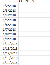
The COUNTIFS function calculates the number of cells across multiple ranges that equals all given conditions.
Function syntax: COUNTIFS(criteria_range1, criteria1, [criteria_range2, criteria2]…)
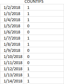
COUNTIFS(B3:B5,"<="&SEQUENCE(MAX(B3:C5)-MIN(B3:C5),,MIN(B3:C5)),C3:C5,">="&SEQUENCE(MAX(B3:C5)-MIN(B3:C5),,MIN(B3:C5)))
becomes
COUNTIFS({43102;43107;43112},{"<=43102";"<=43103";"<=43104";"<=43105";"<=43106";"<=43107";"<=43108";"<=43109";"<=43110";"<=43111";"<=43112";"<=43113"},{43104;43108;43114},{">=43102";">=43103";">=43104";">=43105";">=43106";">=43107";">=43108";">=43109";">=43110";">=43111";">=43112";">=43113"})
and returns
{1; 1; 1; 0; 0; 1; 1; 0; 0; 0; 1; 1}.
Step 7 - Check if number is equal to 0 (zero) meaning no date range is overlapping
COUNTIFS(B3:B5,"<="&SEQUENCE(MAX(B3:C5)-MIN(B3:C5),,MIN(B3:C5)),C3:C5,">="&SEQUENCE(MAX(B3:C5)-MIN(B3:C5),,MIN(B3:C5)))=0
becomes
{1; 1; 1; 0; 0; 1; 1; 0; 0; 0; 1; 1}=0
and returns
{FALSE; FALSE; FALSE; TRUE; TRUE; FALSE; FALSE; TRUE; TRUE; TRUE; FALSE; FALSE}.
Step 8 - Filter no overlapping dates
The FILTER function extracts values/rows based on a condition or criteria.
Function syntax: FILTER(array, include, [if_empty])
FILTER(SEQUENCE(MAX(B3:C5)-MIN(B3:C5),,MIN(B3:C5)),COUNTIFS(B3:B5,"<="&SEQUENCE(MAX(B3:C5)-MIN(B3:C5),,MIN(B3:C5)),C3:C5,">="&SEQUENCE(MAX(B3:C5)-MIN(B3:C5),,MIN(B3:C5)))=0)
becomes
FILTER({43102; 43103; 43104; 43105; 43106; 43107; 43108; 43109; 43110; 43111; 43112; 43113},{FALSE; FALSE; FALSE; TRUE; TRUE; FALSE; FALSE; TRUE; TRUE; TRUE; FALSE; FALSE})
and returns
{43105; 43106; 43109; 43110; 43111}.
Step 9 - Shorten the formula
The LET function lets you name intermediate calculation results which can shorten formulas considerably and improve performance.
Function syntax: LET(name1, name_value1, calculation_or_name2, [name_value2, calculation_or_name3...])
FILTER(SEQUENCE(MAX(B3:C5)-MIN(B3:C5),,MIN(B3:C5)),COUNTIFS(B3:B5,"<="&SEQUENCE(MAX(B3:C5)-MIN(B3:C5),,MIN(B3:C5)),C3:C5,">="&SEQUENCE(MAX(B3:C5)-MIN(B3:C5),,MIN(B3:C5)))=0)
y : B3:C5
x : SEQUENCE(MAX(y)-MIN(y),,MIN(y))
LET(y, B3:C5, x, SEQUENCE(MAX(y)-MIN(y),,MIN(y)), FILTER(x,COUNTIFS(B3:B5,"<="&x,C3:C5,">="&x)=0))
11.2. Find empty dates in a set of date ranges - earlier versions
Array formula in cell B8:
To enter an array formula, type the formula in a cell then press and hold CTRL + SHIFT simultaneously, now press Enter once. Release all keys.
The formula bar now shows the formula with a beginning and ending curly bracket telling you that you entered the formula successfully. Don't enter the curly brackets yourself.
Now copy cell B8 and paste as far as needed to cells below.
11.2.1 How to adjust cell references in the array formula to your worksheet
Cell range $B$3:$B$5 contains the start dates of the date ranges and $C$3:$C$5 contains the end dates.
$B$3:$C$5 contains both the start and end dates of your date ranges. Adjust these accordingly to your worksheet and don't forget to enter the formula as an array formula.
$A$1:A1 is only an expanding cell reference that lets the SMALL function extract the correct date value, you don't need to change it.
11.2.2 Explaining formula in cell B8
Step 1 - Find the earliest date
The MIN function returns the smallest earliest date from cell range $B$3:$C$5. The dollar signs make sure that the cell reference doesn't change when we copy the cell and paste it to the cells below.
MIN($B$3:$C$5)
becomes
MIN({43102, 43104; 43107, 43108; 43112, 43114})
and returns 43102.
Step 2 - Find latest date
The MAX function returns the lates date from cell range $B$3:$C$5
MAX($B$3:$C$5)
becomes
MAX({43102, 43104; 43107, 43108; 43112, 43114})
and returns 43114.
Step 3 - Concatenate results
The ampersand character lets you concatenate strings.
MIN($B$3:$C$5)&":"&MAX($B$3:$C$5)
becomes
43102&":"&43114
and returns "43102:43114".
Step 4- Create a cell reference
The INDIRECT function converts a text string to a working cell reference.
INDIRECT(MIN($B$3:$C$5)&":"&MAX($B$3:$C$5))
becomes
INDIRECT("43102:43114")
and returns 43102:43114.
Step 5 - Create an array of row numbers
ROW(INDIRECT(MIN($B$3:$C$5)&":"&MAX($B$3:$C$5)))
The following formula returns an array of Excel dates needed to extract the missing dates.
ROW(INDIRECT(MIN($B$3:$C$5)&":"&MAX($B$3:$C$5)))
becomes
ROW(INDIRECT(43102&":"&43114))
becomes
ROW(43102:43114)
and returns
{43102; 43103; 43104; 43105; 43106; 43107; 43108; 43109; 43110; 43111; 43112; 43113; 43114}.
Step 6 - which dates are outside the date ranges
The COUNTIFS function returns an array that we can use to extract dates not in date ranges. This particular COUNTIFS function has 4 arguments, however, you can use up to 255 arguments.
COUNTIFS($B$3:$B$5, "<="&ROW(INDIRECT(MIN($B$3:$C$5)&":"&MAX($B$3:$C$5))), $C$3:$C$5, ">="&ROW(INDIRECT(MIN($B$3:$C$5)&":"&MAX($B$3:$C$5))))
becomes
COUNTIFS($B$3:$B$5,{"<=43102"; "<=43103"; "<=43104"; "<=43105"; "<=43106"; "<=43107"; "<=43108"; "<=43109"; "<=43110"; "<=43111"; "<=43112"; "<=43113"; "<=43114"},$C$3:$C$5,{">=43102"; ">=43103"; ">=43104"; ">=43105"; ">=43106"; ">=43107"; ">=43108"; ">=43109"; ">=43110"; ">=43111"; ">=43112"; ">=43113"; ">=43114"})
and returns {1; 1; 1; 0; 0; 1; 1; 0; 0; 0; 1; 1; 1}. This array tells us which dates is in the array and which are not. 1 - yes, 0 (zero) - no. The position in this array is important to identify the corresponding date.
Step 7 - Compare each value in array with 0 (zero)
Value 0 (zero) shows us that the corresponding date is not in the date range so I am now going to compare each value in the array to 0 (zero).
The equal sign lets you compare a value to an array of values, the result is a boolean value TRUE or FALSE.
COUNTIFS($B$3:$B$5, "<="&ROW(INDIRECT(MIN($B$3:$C$5)&":"&MAX($B$3:$C$5))), $C$3:$C$5, ">="&ROW(INDIRECT(MIN($B$3:$C$5)&":"&MAX($B$3:$C$5))))=0
becomes
{1; 1; 1; 0; 0; 1; 1; 0; 0; 0; 1; 1; 1}=0
and returns
{FALSE; FALSE; FALSE; TRUE; TRUE; FALSE; FALSE; TRUE; TRUE; TRUE; FALSE; FALSE; FALSE}.
Step 8 - IF function returns an array of correct dates

The IF function uses the logical values to filter the dates we are looking for.
IF(COUNTIFS($B$3:$B$5, "<="&ROW(INDIRECT(MIN($B$3:$C$5)&":"&MAX($B$3:$C$5))), $C$3:$C$5, ">="&ROW(INDIRECT(MIN($B$3:$C$5)&":"&MAX($B$3:$C$5))))=0, ROW(INDIRECT(MIN($B$3:$C$5)&":"&MAX($B$3:$C$5))))
becomes
IF({FALSE; FALSE; FALSE; TRUE; TRUE; FALSE; FALSE; TRUE; TRUE; TRUE; FALSE; FALSE; FALSE}, {43102; 43103; 43104; 43105; 43106; 43107; 43108; 43109; 43110; 43111; 43112; 43113; 43114})
and returns {FALSE; FALSE; FALSE; 43105; 43106; FALSE; FALSE; 43109; 43110; 43111; FALSE; FALSE; FALSE}
Step 9 - Extract the k-th smallest number (date)
The SMALL function returns dates based on their sizes, the second argument uses an expanding cell reference so that the small function extracts the smallest value in cell B8 and the second smallest in cell B9 and so on.
SMALL(IF(COUNTIFS($B$3:$B$5, "<="&ROW(INDIRECT(MIN($B$3:$C$5)&":"&MAX($B$3:$C$5))), $C$3:$C$5, ">="&ROW(INDIRECT(MIN($B$3:$C$5)&":"&MAX($B$3:$C$5))))=0, ROW(INDIRECT(MIN($B$3:$C$5)&":"&MAX($B$3:$C$5)))), ROWS($A$1:A1))
becomes
SMALL({FALSE; FALSE; FALSE; 43105; 43106; FALSE; FALSE; 43109; 43110; 43111; FALSE; FALSE; FALSE}, ROWS($A$1:A1))
The ROWS function counts the number of rows in a given cell reference, the cell reference used here is a growing cell reference. It contains an absolute and a relative part indicated by the dollar signs.
becomes
SMALL({FALSE; FALSE; FALSE; 43105; 43106; FALSE; FALSE; 43109; 43110; 43111; FALSE; FALSE; FALSE}, 1)
and returns 43105 in cell B8.
Excel formats the number as a date and shows 1/5/2018, see picture below.
12. List dates outside specified date ranges
This article demonstrates how to calculate dates in a given date range (cells B13 and B14) that don't overlap the date ranges specified in cells A3:B10 (Excel Table).
Table of Contents
- List dates outside specified date ranges
- List dates outside specified date ranges - Excel 365
- List empty gaps as date ranges - Excel 365
12.1. List dates outside specified date ranges
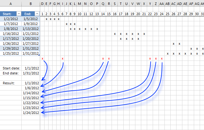
The Excel defined table contains start and end dates for each date range in cell range A3:B10. Cell B13 is the start date and B14 is the end date which are the outer boundaries, obviously, we can't list all dates that ever existed.
The array formula in cell B16 filters all dates between the start and end date and outside the specified date ranges in the Excel defined table.
I made a simple calendar (D3:AH10) next to the Excel defined table (A3:B10) that shows the date ranges and dates not in date ranges (red x). Row 2 contains the days in January 1 to 31, each x below row 2 represents a day in each date range. This makes it much easier to demonstrate and explain what the formula does and also verify the formula result.
Array formula in cell B16:
How to create an array formula
- Copy above array formula
- Press with left mouse button on in formula bar
- Paste array formula (Ctrl + v)
- Press and hold Ctrl + Shift
- Press Enter
How to copy array formula
- Select cell B16
- Copy cell (Ctrl + c)
- Select cell range B17:B25
- Paste (Ctrl + v)
Explaining formula in cell B16
Step 1 - Dynamic cell reference
The INDEX function creates a cell reference based on cell B14 - B13. This cell referenc will in a later step be used to create an array containing a sequence of numbers ranging from 0 to 29. If you change the dates in cell B13 or B14 a new sequence of values is instantly created.
$A$1:INDEX($A:$A,$B$14-$B$13)
becomes
$A$1:INDEX($A:$A,40939-40909)
becomes
$A$1:INDEX($A:$A,30)
and returns
$A$1:$A$30
Step 2 - Create a sequence and add a less than sign to each value in the array
"<="&$B$13+ROW($A$1:INDEX($A:$A,$B$14-$B$13))-1
becomes
"<="&$B$13+ROW($A$1:$A$30)-1
becomes
"<="&$B$13+{0; 1; 2; 3; 4; 5; 6; 7; 8; 9; 10; 11; 12; 13; 14; 15; 16; 17; 18; 19; 20; 21; 22; 23; 24; 25; 26; 27; 28; 29}
becomes
"<="&40909+{0; 1; 2; 3; 4; 5; 6; 7; 8; 9; 10; 11; 12; 13; 14; 15; 16; 17; 18; 19; 20; 21; 22; 23; 24; 25; 26; 27; 28; 29}
becomes
"<="&{40909; 40910; 40911; 40912; 40913; 40914; 40915; 40916; 40917; 40918; 40919; 40920; 40921; 40922; 40923; 40924; 40925; 40926; 40927; 40928; 40929; 40930; 40931; 40932; 40933; 40934; 40935; 40936; 40937; 40938}
and returns
{"<=40909"; "<=40910"; "<=40911"; "<=40912"; "<=40913"; "<=40914"; "<=40915"; "<=40916"; "<=40917"; "<=40918"; "<=40919"; "<=40920"; "<=40921"; "<=40922"; "<=40923"; "<=40924"; "<=40925"; "<=40926"; "<=40927"; "<=40928"; "<=40929"; "<=40930"; "<=40931"; "<=40932"; "<=40933"; "<=40934"; "<=40935"; "<=40936"; "<=40937"; "<=40938"}
Step 3 - Check if dynamic dates are inside the date ranges
The COUNTIFS function calculates the number of cells across multiple ranges that equals all given conditions. The date ranges has a start date and an end date, that means we need two conditions to check if dates are inside the date ranges. The only difference between these two conditions are the less than and greater than signs concatenated to each date.
COUNTIFS(Table1[Start:], "<="&$B$13+ROW($A$1:INDEX($A:$A, $B$14-$B$13))-1, Table1[End:], ">="&$B$13+ROW($A$1:INDEX($A:$A, $B$14-$B$13))-1)
returns
{0; 1; 1; 1; 1; 0; 1; 2; 2; 1; 1; 1; 1; 0; 0; 1; 2; 2; 2; 2; 1; 0; 0; 0; 1; 2; 2; 1; 2; 2}.
Step 4 - Replace 0 (zero) in array with corresponding date
The IF function has three arguments, the first one must be a logical expression. If the expression evaluates to TRUE then one thing happens (argument 2) and if FALSE another thing happens (argument 3).
IF(COUNTIFS(Table1[Start:], "<="&$B$13+ROW($A$1:INDEX($A:$A, $B$14-$B$13))-1, Table1[End:], ">="&$B$13+ROW($A$1:INDEX($A:$A, $B$14-$B$13))-1), "", $B$13+ROW($A$1:INDEX($A:$A, $B$14-$B$13))-1)
becomes
IF({0; 1; 1; 1; 1; 0; 1; 2; 2; 1; 1; 1; 1; 0; 0; 1; 2; 2; 2; 2; 1; 0; 0; 0; 1; 2; 2; 1; 2; 2}, "", {40909; 40910; 40911; 40912; 40913; 40914; 40915; 40916; 40917; 40918; 40919; 40920; 40921; 40922; 40923; 40924; 40925; 40926; 40927; 40928; 40929; 40930; 40931; 40932; 40933; 40934; 40935; 40936; 40937; 40938})
becomes
IF({0; 1; 1; 1; 1; 0; 1; 2; 2; 1; 1; 1; 1; 0; 0; 1; 2; 2; 2; 2; 1; 0; 0; 0; 1; 2; 2; 1; 2; 2}, "", $B$13+ROW($A$1:INDEX($A:$A, $B$14-$B$13))-1)
and returns
{40909; ""; ""; ""; ""; 40914; ""; ""; ""; ""; ""; ""; ""; 40922; 40923; ""; ""; ""; ""; ""; ""; 40930; 40931; 40932; ""; ""; ""; ""; ""; ""}
Step 5 - Extract k-th smallest date
To be able to return a new value in a cell each I use the SMALL function to filter date numbers from smallest to larges
SMALL(IF(COUNTIFS(Table1[Start:], "<="&$B$13+ROW($A$1:INDEX($A:$A, $B$14-$B$13))-1, Table1[End:], ">="&$B$13+ROW($A$1:INDEX($A:$A, $B$14-$B$13))-1), "", $B$13+ROW($A$1:INDEX($A:$A, $B$14-$B$13))-1), ROW(A1))
becomes
SMALL({40909; ""; ""; ""; ""; 40914; ""; ""; ""; ""; ""; ""; ""; 40922; 40923; ""; ""; ""; ""; ""; ""; 40930; 40931; 40932; ""; ""; ""; ""; ""; ""}, ROW(A1))
becomes
SMALL({40909; ""; ""; ""; ""; 40914; ""; ""; ""; ""; ""; ""; ""; 40922; 40923; ""; ""; ""; ""; ""; ""; 40930; 40931; 40932; ""; ""; ""; ""; ""; ""}, 1)
and returns 40909 (1/1/2012) in cell B16.
Step 6 - Replacce errors with blanks
When there are no more values to extract the formula returns errors, the IFERROR function removes the errors and returns blank cells.
IFERROR(SMALL(IF(COUNTIFS(Table1[Start:], "<="&$B$13+ROW($A$1:INDEX($A:$A, $B$14-$B$13))-1, Table1[End:], ">="&$B$13+ROW($A$1:INDEX($A:$A, $B$14-$B$13))-1), "", $B$13+ROW($A$1:INDEX($A:$A, $B$14-$B$13))-1), ROW(A1)), "")
Get excel *.xlsx file
Filter dates outside date ranges.xlsx
12.2. List dates outside specified date ranges - Excel 365
Excel 365 formula in cell B16:
Explaining formula
FILTER($B$13+SEQUENCE($B$14-$B$13)-1,COUNTIFS(Table1[Start:],"<="&$B$13+SEQUENCE($B$14-$B$13)-1,Table1[End:],">="&$B$13+SEQUENCE($B$14-$B$13)-1)=0)
Step 1 - Calculate days in the date range
The minus sign lets you subtract numbers in an Excel formula.
$B$14-$B$13
becomes
40939-40909 equals 30.
Step 2 - Create a sequence of numbers
The SEQUENCE function creates a list of sequential numbers.
Function syntax: SEQUENCE(rows, [columns], [start], [step])
SEQUENCE($B$14-$B$13)-1
becomes
SEQUENCE(30)-1
becomes
{1; 2; 3; 4; 5; 6; 7; 8; 9; 10; 11; 12; 13; 14; 15; 16; 17; 18; 19; 20; 21; 22; 23; 24; 25; 26; 27; 28; 29; 30} - 1
and returns
{0; 1; 2; 3; 4; 5; 6; 7; 8; 9; 10; 11; 12; 13; 14; 15; 16; 17; 18; 19; 20; 21; 22; 23; 24; 25; 26; 27; 28; 29}
Step 3 - Concatenate strings
The plus sign lets you add numbers in an Excel formula. The ampersand character allows you to concatenate values.
"<="&$B$13+SEQUENCE($B$14-$B$13)-1
becomes
"<="&$B$13+{0; 1; 2; 3; 4; 5; 6; 7; 8; 9; 10; 11; 12; 13; 14; 15; 16; 17; 18; 19; 20; 21; 22; 23; 24; 25; 26; 27; 28; 29}
becomes
"<="&{40909; 40910; 40911; 40912; 40913; 40914; 40915; 40916; 40917; 40918; 40919; 40920; 40921; 40922; 40923; 40924; 40925; 40926; 40927; 40928; 40929; 40930; 40931; 40932; 40933; 40934; 40935; 40936; 40937; 40938}
and returns
{"<=40909"; "<=40910"; "<=40911"; "<=40912"; "<=40913"; "<=40914"; "<=40915"; "<=40916"; "<=40917"; "<=40918"; "<=40919"; "<=40920"; "<=40921"; "<=40922"; "<=40923"; "<=40924"; "<=40925"; "<=40926"; "<=40927"; "<=40928"; "<=40929"; "<=40930"; "<=40931"; "<=40932"; "<=40933"; "<=40934"; "<=40935"; "<=40936"; "<=40937"; "<=40938"}
Step 4 - Count dates outside date ranges
The COUNTIFS function calculates the number of cells across multiple ranges that equals all given conditions.
Function syntax: COUNTIFS(criteria_range1, criteria1, [criteria_range2, criteria2]…)
The less than and the larger than characters are logical operators that you can use in the COUNTIFS function. They allow you to count overlapping date ranges with the specified date range in cells B13 and B14.
COUNTIFS(Table1[Start:],"<="&$B$13+SEQUENCE($B$14-$B$13)-1,Table1[End:],">="&$B$13+SEQUENCE($B$14-$B$13)-1)
returns
{0; 1; 1; 1; 1; 0; 1; 2; 2; 1; 1; 1; 1; 0; 0; 1; 2; 2; 2; 2; 1; 0; 0; 0; 1; 2; 2; 1; 2; 2}.
Step 5 - Check if number is equal to 0 (zero)
The equal sign lets you identify if a number in the array is equal to 0 (zero), the result is a boolean value TRUE or FALSE. 0 (zero) means that the date ranges are not overlapping based on the relative position of the number in the array and the position in the Excel Table. In other words, their positions match which makes it easy to extract the corresponding dates.
COUNTIFS(Table1[Start:],"<="&$B$13+SEQUENCE($B$14-$B$13)-1,Table1[End:],">="&$B$13+SEQUENCE($B$14-$B$13)-1)=0
becomes
{0; 1; 1; 1; 1; 0; 1; 2; 2; 1; 1; 1; 1; 0; 0; 1; 2; 2; 2; 2; 1; 0; 0; 0; 1; 2; 2; 1; 2; 2}=0
and returns
{TRUE; FALSE; FALSE; FALSE; FALSE; TRUE; FALSE; FALSE; FALSE; FALSE; FALSE; FALSE; FALSE; TRUE; TRUE; FALSE; FALSE; FALSE; FALSE; FALSE; FALSE; TRUE; TRUE; TRUE; FALSE; FALSE; FALSE; FALSE; FALSE; FALSE}.
Step 6 - Filter dates based on condition
The FILTER function extracts values/rows based on a condition or criteria.
Function syntax: FILTER(array, include, [if_empty])
FILTER($B$13+SEQUENCE($B$14-$B$13)-1,COUNTIFS(Table1[Start:],"<="&$B$13+SEQUENCE($B$14-$B$13)-1,Table1[End:],">="&$B$13+SEQUENCE($B$14-$B$13)-1)=0)
becomes
FILTER($B$13+SEQUENCE($B$14-$B$13)-1,{TRUE; FALSE; FALSE; FALSE; FALSE; TRUE; FALSE; FALSE; FALSE; FALSE; FALSE; FALSE; FALSE; TRUE; TRUE; FALSE; FALSE; FALSE; FALSE; FALSE; FALSE; TRUE; TRUE; TRUE; FALSE; FALSE; FALSE; FALSE; FALSE; FALSE})
becomes
FILTER({40909; 40910; 40911; 40912; 40913; 40914; 40915; 40916; 40917; 40918; 40919; 40920; 40921; 40922; 40923; 40924; 40925; 40926; 40927; 40928; 40929; 40930; 40931; 40932; 40933; 40934; 40935; 40936; 40937; 40938},{TRUE; FALSE; FALSE; FALSE; FALSE; TRUE; FALSE; FALSE; FALSE; FALSE; FALSE; FALSE; FALSE; TRUE; TRUE; FALSE; FALSE; FALSE; FALSE; FALSE; FALSE; TRUE; TRUE; TRUE; FALSE; FALSE; FALSE; FALSE; FALSE; FALSE})
and returns
{40909; 40914; 40922; 40923; 40930; 40931; 40932}
Step 7 - Shorten the formula
The LET function lets you name intermediate calculation results which can shorten formulas considerably and improve performance.
Function syntax: LET(name1, name_value1, calculation_or_name2, [name_value2, calculation_or_name3...])
FILTER($B$13+SEQUENCE($B$14-$B$13)-1,COUNTIFS(Table1[Start:],"<="&$B$13+SEQUENCE($B$14-$B$13)-1,Table1[End:],">="&$B$13+SEQUENCE($B$14-$B$13)-1)=0)
$B$13 is repeated plenty of times in the formula, I will name it y in this example.
SEQUENCE($B$14-$B$13) is also repeated, I am going to name it x.
LET(y, $B$13, x, SEQUENCE($B$14-y)-1, FILTER(y+x, COUNTIFS(Table1[Start:], "<="&y+x, Table1[End:], ">="&y+x)=0))
12.3. List empty gaps as date ranges - Excel 365

The following formulas extract empty gaps between given date ranges specified in the Excel Table located in cells A3:B10.
The formulas returns #CALC error if no empty date ranges exist.
The Excel Table lets you easily add or remove date ranges without the need to adjust cell ranges in the formulas.
Excel 365 formula in cell A17:
Excel 365 formula in cell B17:
Explaining the formula in cell A17
The formulas in cells A17 and B17 check between gaps using the end date to the start date, they are displayed if they don't overlap with the original date ranges meaning they must be an empty space.
=FILTER(FILTER(TOCOL(IF((TRANSPOSE(Table4[End:])+1<=Table4[Start:]-1)*(Table4[Start:]-1>=TRANSPOSE(Table4[End:])+1),TRANSPOSE(Table4[End:])+1,"")),TOCOL(IF((TRANSPOSE(Table4[End:])+1<=Table4[Start:]-1)*(Table4[Start:]-1>=TRANSPOSE(Table4[End:])+1),TRANSPOSE(Table4[End:])+1,""))<>""),COUNTIFS(Table4[Start:],"<="&FILTER(TOCOL(IF((TRANSPOSE(Table4[End:])+1<=Table4[Start:]-1)*(Table4[Start:]-1>=TRANSPOSE(Table4[End:])+1),Table4[Start:]-1,"")),TOCOL(IF((TRANSPOSE(Table4[End:])+1<=Table4[Start:]-1)*(Table4[Start:]-1>=TRANSPOSE(Table4[End:])+1),Table4[Start:]-1,""))<>""),Table4[End:],">="&FILTER(TOCOL(IF((TRANSPOSE(Table4[End:])+1<=Table4[Start:]-1)*(Table4[Start:]-1>=TRANSPOSE(Table4[End:])+1),TRANSPOSE(Table4[End:])+1,"")),TOCOL(IF((TRANSPOSE(Table4[End:])+1<=Table4[Start:]-1)*(Table4[Start:]-1>=TRANSPOSE(Table4[End:])+1),TRANSPOSE(Table4[End:])+1,""))<>""))=0)
Step 1 - Specify reference to the Excel Table
Table4[End:]
Step 2 - Transpose dates
The TRANSPOSE function converts a vertical range to a horizontal range, or vice versa.
Function syntax: TRANSPOSE(array)
TRANSPOSE(Table4[End:])
Step 3 - Add 1
TRANSPOSE(Table4[End:])+1
Step 4 - Subtract dates by 1
Table4[Start:]-1
Step 5 - Check if the end dates are equal to or smaller than the start dates
(TRANSPOSE(Table4[End:])+1)<=(Table[Start:]-1)
Step 6 - Multiply arrays (AND logic)
(TRANSPOSE(Table4[End:])+1<=Table4[Start:]-1)*(Table4[Start:]-1>=TRANSPOSE(Table4[End:])+1)
Step 7 - Replace array with end dates
The IF function returns one value if the logical test is TRUE and another value if the logical test is FALSE.
Function syntax: IF(logical_test, [value_if_true], [value_if_false])
IF((TRANSPOSE(Table4[End:])+1<=Table4[Start:]-1)*(Table4[Start:]-1>=TRANSPOSE(Table4[End:])+1),TRANSPOSE(Table4[End:])+1,"")
Step 8 - Rearrange dates to fit a column
The TOCOL function rearranges values in 2D cell ranges to a single column.
Function syntax: TOCOL(array, [ignore], [scan_by_col])
TOCOL(IF((TRANSPOSE(Table4[End:])+1<=Table4[Start:]-1)*(Table4[Start:]-1>=TRANSPOSE(Table4[End:])+1),TRANSPOSE(Table4[End:])+1,""))
Step 9 - Filter out empty values
The FILTER function extracts values/rows based on a condition or criteria.
Function syntax: FILTER(array, include, [if_empty])
FILTER(TOCOL(IF((TRANSPOSE(Table4[End:])+1<=Table4[Start:]-1)*(Table4[Start:]-1>=TRANSPOSE(Table4[End:])+1),TRANSPOSE(Table4[End:])+1,"")),TOCOL(IF((TRANSPOSE(Table4[End:])+1<=Table4[Start:]-1)*(Table4[Start:]-1>=TRANSPOSE(Table4[End:])+1),TRANSPOSE(Table4[End:])+1,""))<>"")
Step 10 - Count dates
The COUNTIFS function calculates the number of cells across multiple ranges that equals all given conditions.
Function syntax: COUNTIFS(criteria_range1, criteria1, [criteria_range2, criteria2]…)
COUNTIFS(Table4[Start:],"<="&FILTER(TOCOL(IF((TRANSPOSE(Table4[End:])+1<=Table4[Start:]-1)*(Table4[Start:]-1>=TRANSPOSE(Table4[End:])+1),Table4[Start:]-1,"")),TOCOL(IF((TRANSPOSE(Table4[End:])+1<=Table4[Start:]-1)*(Table4[Start:]-1>=TRANSPOSE(Table4[End:])+1),Table4[Start:]-1,""))<>""),Table4[End:],">="&FILTER(TOCOL(IF((TRANSPOSE(Table4[End:])+1<=Table4[Start:]-1)*(Table4[Start:]-1>=TRANSPOSE(Table4[End:])+1),TRANSPOSE(Table4[End:])+1,"")),TOCOL(IF((TRANSPOSE(Table4[End:])+1<=Table4[Start:]-1)*(Table4[Start:]-1>=TRANSPOSE(Table4[End:])+1),TRANSPOSE(Table4[End:])+1,""))<>""))
Step 10 - Filter end dates
Filter end dates whose count is equal to 0 (zero) meaning no overlapping.
FILTER(FILTER(TOCOL(IF((TRANSPOSE(Table4[End:])+1<=Table4[Start:]-1)*(Table4[Start:]-1>=TRANSPOSE(Table4[End:])+1),TRANSPOSE(Table4[End:])+1,"")),TOCOL(IF((TRANSPOSE(Table4[End:])+1<=Table4[Start:]-1)*(Table4[Start:]-1>=TRANSPOSE(Table4[End:])+1),TRANSPOSE(Table4[End:])+1,""))<>""),COUNTIFS(Table4[Start:],"<="&FILTER(TOCOL(IF((TRANSPOSE(Table4[End:])+1<=Table4[Start:]-1)*(Table4[Start:]-1>=TRANSPOSE(Table4[End:])+1),Table4[Start:]-1,"")),TOCOL(IF((TRANSPOSE(Table4[End:])+1<=Table4[Start:]-1)*(Table4[Start:]-1>=TRANSPOSE(Table4[End:])+1),Table4[Start:]-1,""))<>""),Table4[End:],">="&FILTER(TOCOL(IF((TRANSPOSE(Table4[End:])+1<=Table4[Start:]-1)*(Table4[Start:]-1>=TRANSPOSE(Table4[End:])+1),TRANSPOSE(Table4[End:])+1,"")),TOCOL(IF((TRANSPOSE(Table4[End:])+1<=Table4[Start:]-1)*(Table4[Start:]-1>=TRANSPOSE(Table4[End:])+1),TRANSPOSE(Table4[End:])+1,""))<>""))=0)
Step 11 - Shorten the formula
The LET function lets you name intermediate calculation results which can shorten formulas considerably and improve performance.
Function syntax: LET(name1, name_value1, calculation_or_name2, [name_value2, calculation_or_name3...])
FILTER(FILTER(TOCOL(IF((TRANSPOSE(Table4[End:])+1<=Table4[Start:]-1)*(Table4[Start:]-1>=TRANSPOSE(Table4[End:])+1),TRANSPOSE(Table4[End:])+1,"")),TOCOL(IF((TRANSPOSE(Table4[End:])+1<=Table4[Start:]-1)*(Table4[Start:]-1>=TRANSPOSE(Table4[End:])+1),TRANSPOSE(Table4[End:])+1,""))<>""),COUNTIFS(Table4[Start:],"<="&FILTER(TOCOL(IF((TRANSPOSE(Table4[End:])+1<=Table4[Start:]-1)*(Table4[Start:]-1>=TRANSPOSE(Table4[End:])+1),Table4[Start:]-1,"")),TOCOL(IF((TRANSPOSE(Table4[End:])+1<=Table4[Start:]-1)*(Table4[Start:]-1>=TRANSPOSE(Table4[End:])+1),Table4[Start:]-1,""))<>""),Table4[End:],">="&FILTER(TOCOL(IF((TRANSPOSE(Table4[End:])+1<=Table4[Start:]-1)*(Table4[Start:]-1>=TRANSPOSE(Table4[End:])+1),TRANSPOSE(Table4[End:])+1,"")),TOCOL(IF((TRANSPOSE(Table4[End:])+1<=Table4[Start:]-1)*(Table4[Start:]-1>=TRANSPOSE(Table4[End:])+1),TRANSPOSE(Table4[End:])+1,""))<>""))=0)
x - TRANSPOSE(Table[End:])+1
y - Table[Start:]-1
z - TOCOL(IF((x<=y)*(y>=x),x,""))
w - TOCOL(IF((x<=y)*(y>=x),y,""))
q - FILTER(z,z<>"")
LET(x,TRANSPOSE(Table[End:])+1,y,Table[Start:]-1,z,TOCOL(IF((x<=y)*(y>=x),x,"")),w,TOCOL(IF((x<=y)*(y>=x),y,"")),q,FILTER(z,z<>""),FILTER(q,COUNTIFS(Table[Start:],"<="&FILTER(w,w<>""),Table[End:],">="&q)=0))
Overlapping category
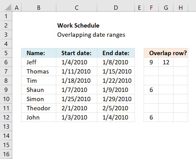
This article demonstrates a formula that points out row numbers of records that overlap the current record based on a […]
Excel categories
23 Responses to “Working with overlapping date ranges”
Leave a Reply
How to comment
How to add a formula to your comment
<code>Insert your formula here.</code>
Convert less than and larger than signs
Use html character entities instead of less than and larger than signs.
< becomes < and > becomes >
How to add VBA code to your comment
[vb 1="vbnet" language=","]
Put your VBA code here.
[/vb]
How to add a picture to your comment:
Upload picture to postimage.org or imgur
Paste image link to your comment.
typo??
INDEX($A:$A, $B$14-$B$13) --> INDEX($A:$A, $B$14-$B$13+1)
aMareis,
I don´t think so. Can you explain why?
If B9=2012-01-30 and B10=2012-01-30 then ????
Your result omit 2012-01-31.
Thanks a tonne, Oscar. It took me about 8 hours to work through this formula piece by piece, play with it, and come to grips with its basics. Your example was clear and very useful, and this has allowed me to do big, very useful data analysis for the company that employs me. It applies to thousands of people. You're an unsung hero.
Actually just realized that I really need what you said you'd "save for a future post" (actually total number of overlapping dates). I guess I'll try to figure that out. Still... couldn't have gotten this close without you.
NC,
read this post:
https://www.get-digital-help.com/count-overlapping-days-across-multiple-date-ranges/
[…] NC asks: […]
[…] The value in cell A11 is wrong because of this, only 9 dates are overlapped. There is a formula for this scenario also but I'll save it for a future post. […]
in the above eg. if now i have multiple date range ( ie.(A8:B8) is now (A8:B20) or more and the range (A2:B4 ) is now (A2: B100) , then how to calculate overlap for each row (A8:B8), (A9:B9) and so on
Also this needs to account for workdays only, and the data in (A8:B8)... are dynamic
Hi Oscar,
Thanks for your knowledge sharing and really helpful!
You have mentioned the overlapping date within a single month. My question is how can we highlight the overlapping dates for 2 months. Kindly find the details below for your reference.
Date Format is in (MM/DD/YYYY)
Start - 03/28/2016 - End - 04/05/2016
Start - 04/25/2016 - End - 05/10/2016
I need your help in this issue. It will be great if I get the solution for this and the same will reduce my work upto 50%. Requesting you to provide me the solution for my query.
Regards
Sam Fredy. P
Hi Oscar,
Please help. Awaiting for your positive reply.
Regards
Sam
Hi Oscar,
Pls help me for my query.
Regards
Sam
i don't know but it does not work for me for 180 lines of range dates can you please help me ?
Hey! Awesome article. Instead of finding the most overlapped date, how would you find the largest number of overlaps (i.e. count of the overlaps on the date instead of the date)?
My question is probably better suited here (I had initially posted in it Part 1). For this example, I want to find the maximum number of overlaps that occurred with a set of date ranges (i.e. in this example above, it would be four (or another way of looking at it is I want the Max value of Row 12).
This is so close to what I want. However, what I would LOVE to see in column "R" is the total number of days that one date overlaps all others.
For instance, the date range on row has 2 days that overlap 3 other date ranges. I would like to see the formula for calculating that 2 days in Column "R"
Then I can do a "Countifs" for the number days that overlap with other date ranges where the same "resource" has been assigned.
Is this possible?
This formula is almost perfect for what I need. Is there a way to add an "If" statement so that the overlap will calculate dependent on an email address. I need to calculate overlap by person for 9000 people.
Christyn Lewandowski,
great question. I have added more content to this article that answers your question.
What about the opposite? I'd like a sum of dates that are NOT overlapping. For example: a ticket's dates of validity compared to dates of actual use, when some of the days were not included with the ticket.
Ticket start: 01/01/2010 Ticket end 01/05/2010 Actual use start: 01/04/2010 Actual use end: 01/07/2010. The result should be 2, because they used the service on Jan 6 and Jan 7, when those dates were not covered by their ticket.
Thanks!!!!!
Excel Noob,
Formula in cell F3:
=MEDIAN(B3,C3+1,E3+1) - MEDIAN(B3,C3+1,D3)
Units contained in a range that overlap another range
Oscar, this is amazing stuff! I did have a follow-up question on this method. I have data that decades - I need to calculate the quantity of days that overlap for each row (or project). For example, if I have four concurrent projects, each one as a row, I need to calculate the total quantity of days that the other three projects might overlap. This figure would need to be calculated for each row. How might you recommend proceeding? Thank you for your time!
Thank you so much for all your posts.
am trying to count number of unique overlap days between a start and end date and a range of start and end dates, it is I think what you referred to as a future post - but that calculates all the overlapped dates, am only interested in one set of overlapped dates.
is that a relatively easy ask? hope so.
Thanks - sfd