How to compare two data sets
Table of Contents
- How to compare two data sets - Excel Table and autofilter
- Filter shared records from two tables
- Filter values that exists in all three columns
- Extract shared values between two columns
- Extract shared values between two columns - Excel 365
- Extract shared values between two columns (case sensitive)
- Filter common values from three separate columns
- Filter values in common between two multi-column cell ranges - Excel 365
- Filter values in common between two multi-column cell ranges - Excel 2019
- Filter values in common between two multi-column cell ranges - earlier versions
- Filter values in common between two multi-column cell ranges - UDF
1. How to compare two data sets - Excel Table and autofilter

This article demonstrates how to quickly compare two data sets in Excel using a formula and Excel defined Tables. The formula will return TRUE if a record is found in the other data set and FALSE if not.
The image above shows you the first data set: Table1 The image below shows you the second data set: Table2

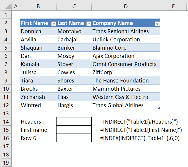
Excel defined tables has many advantages, one is that you only need to enter a formula in one cell and Excel automatically enters the formula in the remaining cells in the same column.
Another one is that it expands accordingly when new data is added, no need to adjust the cell references. You can also easily filter the data using the arrows in the top row of the Excel table.
How to convert a data set to an Excel defined Table:
-
- Select a cell in the data set.
- Press CTRL + T.
- Press with left mouse button on checkbox if your data set has headers.
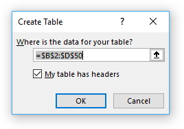
- Press with left mouse button on OK.
Type the following formula in the next column adjacent to the Excel defined Table:
The Excel defined Table will automatically expand shown in the image below and enter the formula in all cells below in that column.

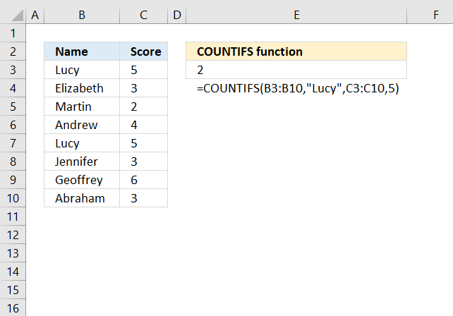
Explaining formula in cell E3
The COUNTIFS function calculates the number of cells across multiple ranges that equals all given conditions. There is a criteria range and a condition forming a pair, our Excel table has three columns so wee need three pairs in order to find matching records in the other table.
COUNTIFS(criteria_range1, criteria1, [criteria_range2, criteria2]…)
Step 1 - Build COUNTIFS function
The first argument is a cell reference to the entire column in table2 and the second argument is a cell reference to the cell on the same row as the formula but in column GivenName. Excel automatically enters these cell references (structured references) if you select the cells with your mouse when you build the formula.
You can also type the table name and column name in brackets, the formula bar will guide you in this process.
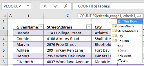
COUNTIFS(Table2[GivenName],[@GivenName]
Complete the function by adding the remaining cell references to the COUNTIFS function.
COUNTIFS(Table2[GivenName],[@GivenName],Table2[StreetAddress],[@StreetAddress],Table2[City],[@City])
Step 2 - Logical expression
The COUNTIFS function returns a number representing how many records that match the current record in the other table. A number larger than zero indicates that there is at least one match.
COUNTIFS(Table2[GivenName],[@GivenName],Table2[StreetAddress],[@StreetAddress],Table2[City],[@City])>0
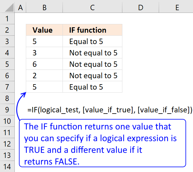
TRUE - At least one match.
FALSE - No match.
Filter records occuring in both tables
- Select sheet 1 (Table1)
- Press with left mouse button on black arrow in column Compare
- Disable FALSE
- Press with left mouse button on OK.

The image below shows a filtered table with records that exists in both tables.

Filter records existing in only one table
- Select a sheet
- Press with left mouse button on black arrow in column Compare
- Enable only FALSE
- Press with left mouse button on OK.
Table1

Table2

2. Filter shared records from two tables
I will in this section demonstrate a formula that extracts common records (shared records) from two data sets in Excel. I have demonstrated how to compare two columns and today I want to show you how to filter records that exists in both tables.
You can also use conditional formatting to highlight shared records. If you are looking for records that exist only in one out of two tables then read this article: Filter records occurring in only one table
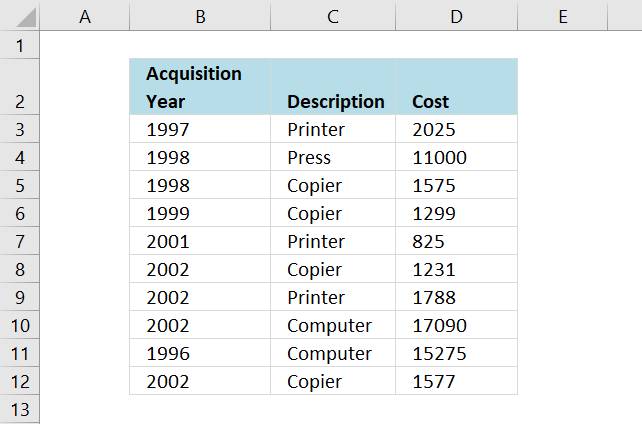
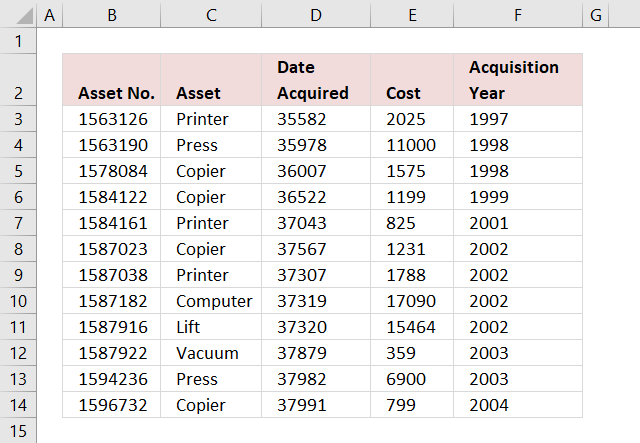
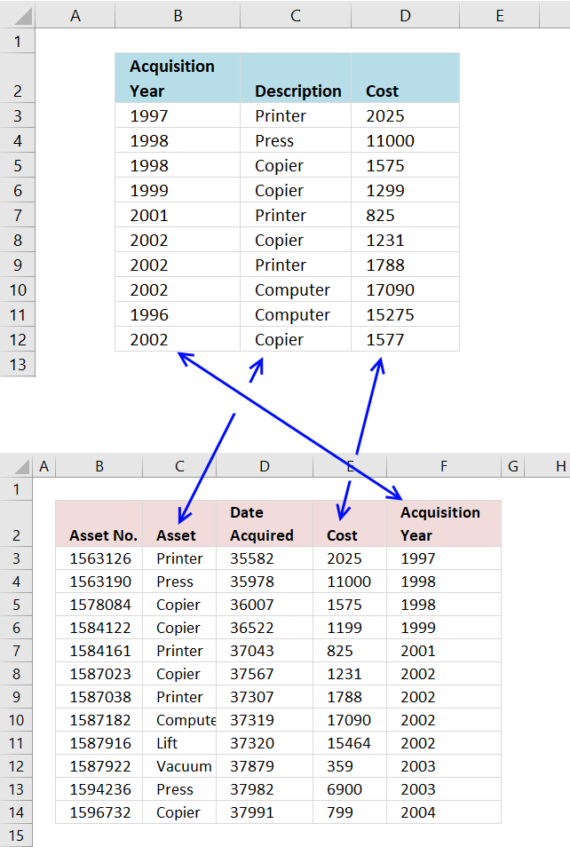
The first data set is in worksheet: List 1, see image above. The second data set is in worksheet: List 2, see image below. These two data sets have three columns each that I want to compare. One column has a different header name.
The columns I am going to compare are these:
- List 1 : Description - List 2 : Asset
- List 1 : Cost - List 2 : Cost
- List 1 : Acquisition year - List 2 : Acquisition year
The following picture shows the columns I am going to compare. Keep in mind that records must be exactly the same in both data tables to be filtered, except that letter case may differ.
COUNTIFS is the core in the formula I will construct, it is here all the comparisons will take place. It is important to understand what is going on so you can use this technique to create your own powerful array formulas.
The COUNTIFS function may have up to 255 arguments leaving you to compare up to 127 columns, however, if you have that many columns to compare perhaps a UDF (User defined function) is a better option. Array formulas are often quite slow dealing with lots of data.
COUNTIFS(criteria_range1,criteria1, criteria_range2, criteria2...)
Counts the number of cells specified by a given set of conditions or criteria
Here are the cell ranges that I am going to use in the COUNTIFS function:
List 2 - Aquisition year - 'List 2'!$F$3:$F$14
List 1 - Aquisition year - 'List 1'!$B$3:$B$12
List 2 - Asset - 'List 2'!$C$3:$C$14
List 1 - Description - 'List 1'!$C$3:$C$12
List 2 - Cost - 'List 2'!$E$3:$E$14
List 1 - Cost - 'List 1'!$D$3:$D$12
COUNTIFS('List 2'!$F$3:$F$14,'List 1'!$B$3:$B$12,'List 2'!$C$3:$C$14,'List 1'!$C$3:$C$12,'List 2'!$E$3:$E$14,'List 1'!$D$3:$D$12)
Is it important to begin with the second data set in the first argument? No, you can begin with the first data set if you like, remember to change cell reference in the INDEX function so you fetch the right values.
With the COUNTIFS function complete we can now construct the array formula.
Formulas
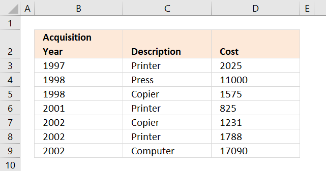
The image above shows the third worksheet named: Common records
Excel 365 dynamic array formula in cell B3:
Array formula in cell B3:
How to create an array formula
- Select cell B3
- Press with left mouse button on in formula bar

- Copy the array formula above and paste to formula bar
- Press and hold Ctrl + Shift simultaneously
- Press Enter
- Release all keys
You can check using the formula bar that you did above steps right, Excel tells you if a cell contains an array formula by surrounding the formula with a beginning and ending curly brackets, like this: {=array_formula}.
Don't enter these characters yourself they show up automatically if you did above steps correctly.
Copy cell B3 and paste it to the right as far as needed. Copy cell B3:D3 and paste down as far as needed.
Explaining the array formula in cell B3
You can easily examine a formula (or array formula) that you don't understand, select the cell containing the formula. Go to tab "Formulas", press with left mouse button on "Evaluate Formula".
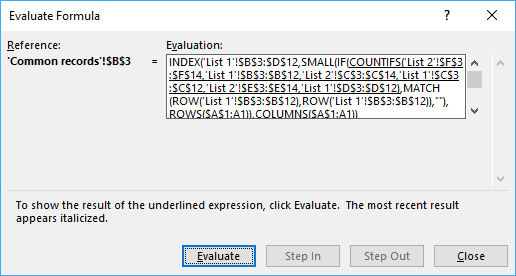
The "Evaluate" button above lets you go to the next "calculation" step.
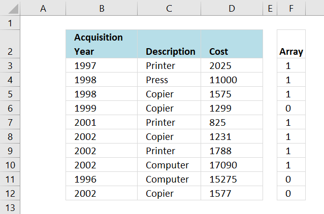
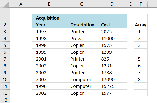
Step 1 - Find common records
COUNTIFS('List 2'!$F$3:$F$14,'List 1'!$B$3:$B$12,'List 2'!$C$3:$C$14,'List 1'!$C$3:$C$12,'List 2'!$E$3:$E$14,'List 1'!$D$3:$D$12)
returns this array: {1, 1, 1, 0, 1, 1, 1, 1, 0, 0}
The array is shown in column F below, the first 1 in the array means that the three corresponding values on row 3 (B3, C3 and D3) have a match somewhere on the other data table, on the same row.
Recommended articles
Checks multiple conditions against the same number of cell ranges and counts how many times all criteria are met.
Step 2 - Return corresponding relative row numbers
IF(COUNTIFS('List 2'!$F$3:$F$14,'List 1'!$B$3:$B$12,'List 2'!$C$3:$C$14,'List 1'!$C$3:$C$12,'List 2'!$E$3:$E$14,'List 1'!$D$3:$D$12),MATCH(ROW('List 1'!$B$3:$B$12),ROW('List 1'!$B$3:$B$12)),"")
returns {1,2,3,"",5,6,7,"",""}
The image below shows you relative row numbers for records that exist on the other data table.
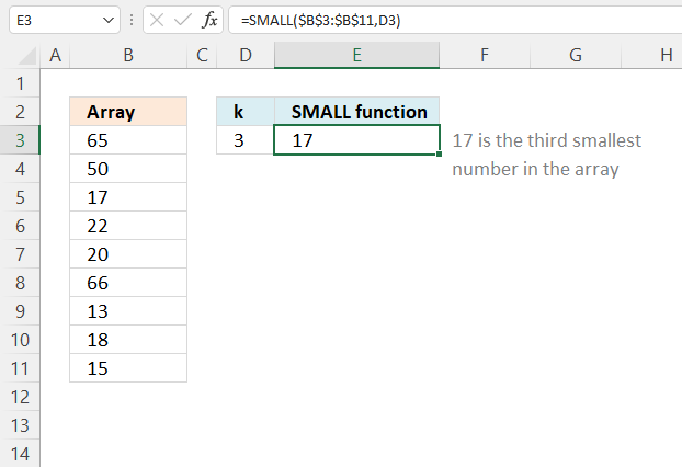
Now it is really easy for the INDEX function to fetch the values it need, first I need to make this array formula return a single number. The SMALL function helps me with that.
Recommended articles
Checks if a logical expression is met. Returns a specific value if TRUE and another specific value if FALSE.
Step 3 - Return the k-th smallest value
I don't want the SMALL function to extract the same value in every cell, I want it to change so a new row number is extracted in the cell below. This is repeated in every new cell below until all values have been extracted.
SMALL({1,2,3,"",5,6,7,"",""}, ROWS($A$1:A1))
returns 1.
The ROWS function return the number of rows a certain cell range has. If that cell range expands every time I copy the formula to new cells below, the ROWS function will return the old number + 1.
In cell B3 ROWS($A$1:A1) returns 1. In cell B4 it changes to ROWS($A$1:A2) and returns 2. Read more about absolute and relative cell references here.
Why use the ROWS function and not ROW? If you insert new rows above the formula, the ROW function will return the wrong value because the relative cell reference changed. It will change in the ROWS function as well but so will also the absolute cell reference.
Recommended articles
The SMALL function lets you extract a number in a cell range based on how small it is compared to the other numbers in the group.
Step 4 - Return a value of the cell at the intersection of a particular row and column
INDEX('List 1'!$B$3:$D$12,SMALL(IF(COUNTIFS('List 2'!$F$3:$F$14,'List 1'!$B$3:$B$12,'List 2'!$C$3:$C$14,'List 1'!$C$3:$C$12,'List 2'!$E$3:$E$14,'List 1'!$D$3:$D$12),MATCH(ROW('List 1'!$B$3:$B$12),ROW('List 1'!$B$3:$B$12)),""),ROWS($A$1:A1)),COLUMNS($A$1:A1))
returns 1997 in cell B3.
Recommended articles
Gets a value in a specific cell range based on a row and column number.
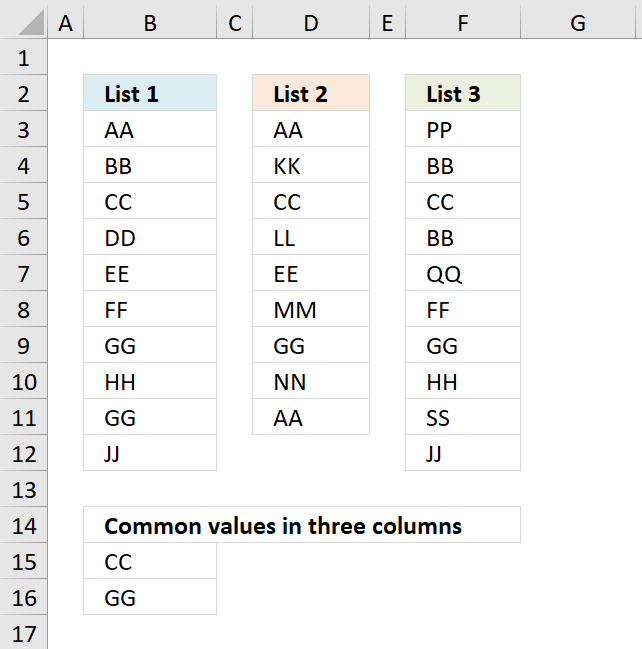
3. Filter values that exists in all three columns

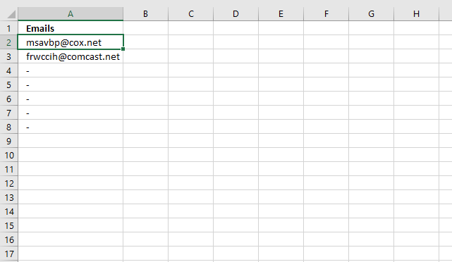
This article explains how to extract values that exist in three different columns, they must occur in each of the three columns in order to be extracted. The example demonstrated in this article uses email addresses but you can use any kind of value.
The image above shows three different columns all containing email addresses, here is the question that inspired me to do this article.
This is close to what I need. I have three lists of email addresses. If an email address appears in all three (not two out of three) lists then place it in the duplicate column. Also, I need all three named ranges to be dynamic.
Named ranges
Named ranges allow you to create dynamic cell ranges that automatically grows when new data is added, this way you won't need to adjust cell references in formulas each time new values are added.
There are three columns so we need three different named ranges are necessary, here are the steps to create a named range:
- Go to tab "Formulas" on the ribbon.
- Press with left mouse button on "Name Manager" button.

- Press with left mouse button on "New..." button.
- Name the named range based on the data below.
- Use the first formula below.
- Press with left mouse button on OK button.
- Repeat above steps so in total three named ranges are created, they are Email_Address, Email_Address2, Email_Address3.
Named range: Email_Address
Formula:
The COUNTA function counts the number of cells in column A that are not empty. The INDEX function uses that number to create a cell reference to the last not empty cell.
The named range concatenates the first cell reference and the second cell reference and creates a single cell reference to a cell range. If a new value is added the named range expands automatically, and it shrinks if the last value is deleted.
The disadvantage with this formula is that it doesn't take blank cells into account. If the cell range is not contiguous meaning there are blanks between values than the named range returns a smaller cell reference than required.
This named range formula takes care of that problem:
=Sheet1!$A$2:INDEX($A:$A,MATCH("ZZZZZZZZZZZZZZZZ",$A:$A))
Named range: Email_address2
Formula:
Named range: Email_address3
Formula:
Sheet 2 - Duplicate column
Array formula in cell A2:
How to enter an array formula
- Select cell A2
- Press with left mouse button on in formula bar
- Copy/Paste or type above array formula
- Press and hold Ctrl + Shift
- Press Enter
- The formula is now surrounded by curly brackets {=array_formula}
How to copy array formula
- Select cell A2
- Copy (Ctrl + c)
- Select cell range A3:A8
- Paste (Ctrl + v)
Explaining array formula in cell A2, sheet2
Step 1 - Identify email adresses in Email address 2 column that exists in Email address 1 column
The COUNTIF function counts cells based on a condition or multiple conditions. COUNTIF(range, criteria) In this case the function contains multiple conditions and if the number in the array is larger than 0 (zero) then the value exists in the other column.
COUNTIF(Email_address2, Email_Address)
becomes
COUNTIF({"[email protected]"; "[email protected]"; "[email protected]"; "[email protected]"; "[email protected]"; "[email protected]"; "[email protected]"; "[email protected]"; "[email protected]"; "[email protected]"; "[email protected]"; "[email protected]"; "[email protected]"; "[email protected]"; "[email protected]"}, {"[email protected]"; "[email protected]"; "[email protected]"; "[email protected]"; "[email protected]"; "[email protected]"; "[email protected]"; "[email protected]"; "[email protected]"; "[email protected]"; "[email protected]"; "[email protected]"; "[email protected]"; "[email protected]"; "[email protected]"; "[email protected]"; "[email protected]"; "[email protected]"; "[email protected]"; "[email protected]"})
and returns
{1; 0; 0; 0; 0; 0; 1; 0; 0; 0; 0; 0; 0; 0; 0; 0; 0; 0; 1; 0}
Step 2 - Identify email adresses in Email address 3 column that exists in Email address 1 column
This part compares the first column with the third column.
COUNTIF(Email_address3, Email_Address)
becomes
COUNTIF({"[email protected]"; "[email protected]"; "[email protected]"; "[email protected]"; "[email protected]"; "[email protected]"; "[email protected]"; "[email protected]"; "[email protected]"; "[email protected]"; "[email protected]"; "[email protected]"; "[email protected]"; "[email protected]"; "[email protected]"; "[email protected]"; "[email protected]"}, {"[email protected]"; "[email protected]"; "[email protected]"; "[email protected]"; "[email protected]"; "[email protected]"; "[email protected]"; "[email protected]"; "[email protected]"; "[email protected]"; "[email protected]"; "[email protected]"; "[email protected]"; "[email protected]"; "[email protected]"; "[email protected]"; "[email protected]"; "[email protected]"; "[email protected]"; "[email protected]"})
and returns
{1; 0; 0; 0; 0; 0; 1; 0; 0; 0; 0; 0; 0; 0; 0; 0; 0; 0; 0; 0}
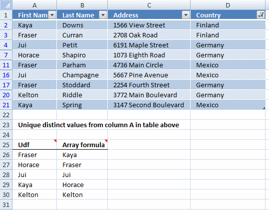
Step 3 - Extract only unique distinct email addresse from Email Address 1 column
The NOT function changes booolean value TRU to FALSE and vice versa.
The COUNTIF function makes sure that only one instance of each value is returned.
NOT(COUNTIF($A$1:A1, Email_Address))
becomes
COUNTIF("Emails", {"[email protected]"; "[email protected]"; "[email protected]"; "[email protected]"; "[email protected]"; "[email protected]"; "[email protected]"; "[email protected]"; "[email protected]"; "[email protected]"; "[email protected]"; "[email protected]"; "[email protected]"; "[email protected]"; "[email protected]"; "[email protected]"; "[email protected]"; "[email protected]"; "[email protected]"; "[email protected]"})
and returns
{TRUE; TRUE; TRUE; TRUE; TRUE; TRUE; TRUE; TRUE; TRUE; TRUE; TRUE; TRUE; TRUE; TRUE; TRUE; TRUE; TRUE; TRUE; TRUE; TRUE}
Step 4 - Multiply all arrays
This part of the formula applies AND logic between the arrays, this is done by multiplying the arrays.
COUNTIF(Email_address2, Email_Address)*COUNTIF(Email_address3, Email_Address)*NOT(COUNTIF($A$1:A1, Email_Address))
becomes
{1; 0; 0; 0; 0; 0; 1; 0; 0; 0; 0; 0; 0; 0; 0; 0; 0; 0; 1; 0} * {1; 0; 0; 0; 0; 0; 1; 0; 0; 0; 0; 0; 0; 0; 0; 0; 0; 0; 0; 0} * {TRUE; TRUE; TRUE; TRUE; TRUE; TRUE; TRUE; TRUE; TRUE; TRUE; TRUE; TRUE; TRUE; TRUE; TRUE; TRUE; TRUE; TRUE; TRUE; TRUE}
and returns
{1; 0; 0; 0; 0; 0; 1; 0; 0; 0; 0; 0; 0; 0; 0; 0; 0; 0; 0; 0}
Step 5 - Find relative position of the first email address existing in all three lists
The MATCH function returns the relative position of a specific value in a cell range or array.
MATCH(1, COUNTIF(Email_address2, Email_Address)*COUNTIF(Email_address3, Email_Address)*NOT(COUNTIF($A$1:A1, Email_Address)), 0)
becomes
MATCH(1, {1; 0; 0; 0; 0; 0; 1; 0; 0; 0; 0; 0; 0; 0; 0; 0; 0; 0; 0; 0}, 0)
and returns 1.
Step 6 - Return a value of the cell at the intersection of a particular row and column
The INDEX function returns a value from a cell range or aray based on a row and column number.
INDEX(Email_Address, MATCH(1, COUNTIF(Email_address2, Email_Address)*COUNTIF(Email_address3, Email_Address)*NOT(COUNTIF($A$1:A1, Email_Address)), 0))
becomes
INDEX(Email_Address, 1)
becomes
INDEX({"[email protected]"; "[email protected]"; "[email protected]"; "[email protected]"; "[email protected]"; "[email protected]"; "[email protected]"; "[email protected]"; "[email protected]"; "[email protected]"; "[email protected]"; "[email protected]"; "[email protected]"; "[email protected]"; "[email protected]"; "[email protected]"; "[email protected]"; "[email protected]"; "[email protected]"; "[email protected]"}, 1)
and returns [email protected] in cell A2.
4. Extract shared values between two columns
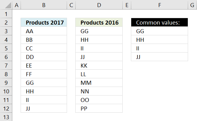
The picture above shows two lists, one in column B and one in column D. The array formula in cell F3 extracts values that both lists have.
Array formula in cell F3:
In this case GG, HH, II, and JJ are in both lists, see the picture below.
The formula above can only compare two columns, however, the lists don't have to be the same size.
If you need to compare two different multicolumn cell ranges, read the following article:
Recommended articles
The image above shows an array formula in cell B12 that extracts values shared by cell range B2:D4 (One) and […]
4.1 How to create an array formula
- Select cell F3
- Press with left mouse button on in formula bar
- Copy and paste the array formula above to formula bar
- Press and hold Ctrl + Shift simulateously
- Press Enter
- Release all keys
You can check using the formula bar that you did above steps right, excel tells you if a cell contains an array formula by surrounding the formula with a beginning and ending curly brackets, like this: {=array_formula}.
Don't enter these characters yourself they show up automatically if you did above steps correctly.
Recommended articles

Array formulas allows you to do advanced calculations not possible with regular formulas.
4.2 How to copy array formula
Copy cell F3 and paste it to cells below as far as needed.
4.3 Explaining array formula in cell C2
You can easily examine a formula (or array formula) that you don't understand, select the cell containing the formula. Go to tab "Formulas", press with left mouse button on "Evaluate Formula".
The "Evaluate" button above lets you see the next "calculation" step.
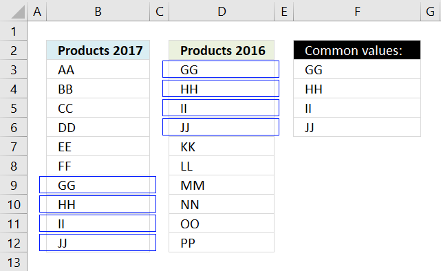
Step 1 - Compare cell range 1 with cell range 2
The COUNTIF function lets you compare values if you enter it as an array formula and use multiple values as criteria. COUNTIF(range, criteria)
COUNTIF($D$3:$D$12, $B$3:$B$12)
The array is shown in column H below.
This tells us that AA exists 0 (zero) times in cell range D3:D12,
BB - 0, CC - 0, DD - 0, EE-0, FF - 0
but GG is found once in cell range D3:D12 and so are HH, II, JJ.
Recommended articles

Counts the number of cells that meet a specific condition.
Step 2 - Check if value exists, if so return corresponding position in array
IF({0; 0; 0; 0; 0; 0; 1; 1; 1; 1}, MATCH(ROW($B$3:$B$12),ROW($B$3:$B$12)), "")
The array is shown in column H below.
Recommended articles
Checks if a logical expression is met. Returns a specific value if TRUE and another specific value if FALSE.
Step 3 - Extract k-th smallest value
Until now we have been working with an array of values but excel allows us to only display one value per cell (That is not entirely true, as of Excel 2016 you can display all values in an array in one cell)
To extract a specific number from an array I use the SMALL function.
SMALL(IF(COUNTIF($D$3:$D$12, $B$3:$B$12), MATCH(ROW($B$3:$B$12),ROW($B$3:$B$12)), ""), ROWS($A$1:A1))
returns number 7, SMALL function ignores blanks and letters.
Recommended articles
The SMALL function lets you extract a number in a cell range based on how small it is compared to the other numbers in the group.
Step 4 - Return corresponding value
INDEX($B$3:$B$12, SMALL(IF(COUNTIF($D$3:$D$12, $B$3:$B$12), MATCH(ROW($B$3:$B$12),ROW($B$3:$B$12)), ""), ROWS($A$1:A1)))
returns GG in cell F3.
When you copy cell F3 and paste it to cell F4 the relative cell references changes. ROWS($A$1:A1) becomes ROWS($A$1:A2) and returns 2 in cell F4.
The second smallest value is then extracted from the array which is 8. The value in cell range B3:B12 in row 8 is HH. HH is returned the value returned to F4.
Recommended articles
Gets a value in a specific cell range based on a row and column number.
Get excel sample file for this tutorial
common-values1.xlsx
(Excel 2007 Workbook *.xlsx and later versions)
5. Extract shared values between two columns - Excel 365

This Excel 365 dynamic array formula extracts values from cell range B3:B12 only if they also exist in cell range D3:D12.
Formula in cell F3:
5.1 Explaining formula
Step 1 - Find values in common
The COUNTIF function lets you compare values if you enter it as an array formula and use multiple values as criteria.
COUNTIF(range, criteria)
COUNTIF($D$3:$D$12, $B$3:$B$12)
returns {0; 0; 0; 0; 0; 0; 1; 1; 1; 1}
Step 2 - Extract values
The FILTER function extracts values/rows based on a condition or criteria.
FILTER(array, include, [if_empty])
FILTER($B$3:$B$12,COUNTIF($D$3:$D$12, $B$3:$B$12))
becomes
FILTER($B$3:$B$12, {0; 0; 0; 0; 0; 0; 1; 1; 1; 1})
and returns
{"GG"; "HH"; "II"; "JJ"}
6. Extract shared values between two columns - case sensitive

This formula shown in the image above extracts values in the first cell range if they also exist in the second cell range, upper and lower letters are also evaluated.
Excel 365 dynamic array formula in cell F3:
6.1 Explaining formula
Step 1 - Rearrange values from vertical to horizontal
The TRANSPOSE function converts a vertical range to a horizontal range, or vice versa.
TRANSPOSE(array)
TRANSPOSE(D3:D12)
returns {"GG", "HH", "II", ... , "aa"}.
Step 2 - Compare values based on upper and lower letters
The EXACT function performs a case sensitive comparison between values.
EXACT(value1, value2)
EXACT(B3:B12,TRANSPOSE(D3:D12))
returns an array shown in the image below. I have added the corresponding values from both cell ranges and highlighted values that exist in both cell ranges.

Step 3 - Convert boolean values
The asterisk lets you multiply numbers in an Excel formula, it also lets you convert boolean values to their numerical equivalents.
TRUE -> 1
FALSE -> 0 (zero)
EXACT(B3:B12,TRANSPOSE(D3:D12))*1
becomes
{FALSE,FALSE,FALSE, ... ,FALSE}*1
and returns

Step 4 - Create an array containing 1's
The ROW function returns the corresponding row number in a cell reference or multiple row numbers if a cell range reference is used.
ROW(reference)
ROW(B3:B12)^0
becomes
{3; 4; 5; 6; 7; 8; 9; 10; 11; 12}^0
and returns
{1; 1; 1; 1; 1; 1; 1; 1; 1; 1}.
Step 5 - Sum numbers row-wise
The MMULT function calculates the matrix product of two arrays, an array as the same number of rows as array1 and columns as array2.
MMULT(array1, array2)
MMULT(EXACT(B3:B12,TRANSPOSE(D3:D12))*1,ROW(B3:B12)^0)
becomes
MMULT({0,0,0, ... ,0},{1; 1; 1; 1; 1; 1; 1; 1; 1; 1})
and returns
{0; 0; 0; 0; 0; 0; 0; 1; 1; 1}.
Step 6 - Filter values based on array
The FILTER function extracts values/rows based on a condition or criteria.
FILTER(array, include, [if_empty])
FILTER($B$3:$B$12,MMULT(EXACT(B3:B12,TRANSPOSE(D3:D12))*1,ROW(B3:B12)^0))
returns
{"HH"; "II"; "JJ"}.
7. Filter common values from three separate columns
The image above demonstrates a formula in cell B15 that extracts values if they exist in all three cell ranges B3:B12, D3:D12, and F3:F12.
Array formula in B15:
Copy cell B15 and paste it to cells below as far as necessary.
To enter an array formula, type the formula in a cell then press and hold CTRL + SHIFT simultaneously, now press Enter once. Release all keys.
The formula bar now shows the formula with a beginning and ending curly bracket telling you that you entered the formula successfully. Don't enter the curly brackets yourself.
Explaining formula in cell B15
Step 1 - Prevent duplicates in the list
The COUNTIF function counts values based on a condition or criteria. The first argument $B$14:B14 expands as the cell is copied to cells below. This makes the formula aware of displayed values above the current cell.
COUNTIF($B$14:B14, $B$3:$B$12)
returns {0;0;0... ;0}
Step 2 - Find position of value in array
The MATCH function returns a number representing the position of a value in a list.
MATCH(0,COUNTIF($B$14:B14,$B$3:$B$12)+(((COUNTIF($D$3:$D$11,$B$3:$B$12)>0)+(COUNTIF($F$3:$F$12,$B$3:$B$12)>0))<>2),0)
returns 3.
Step 3 - Return value
The INDEX function returns a value based on a row and column number.
INDEX($B$3:$B$12, MATCH(0, COUNTIF($B$14:B14, $B$3:$B$12)+IF(((COUNTIF($D$3:$D$11, $B$3:$B$12)>0)+(COUNTIF($F$3:$F$12, $B$3:$B$12)>0))=2, 0, 1), 0))
returns "CC" in cell B15.
Get Excel *.xlsx file
Common values in three columns.xlsx
8. Filter common values between two nonadjacent cell ranges - Excel 365

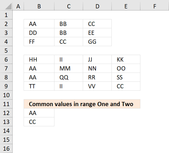
This example demonstrates a short dynamic array formula that works only in Excel 365. It compares two cell ranges B2:D4 and B6:E9 and extracts values in common between these two cell ranges.
The formula returns values to cell G3 and cells below automatically, Microsoft calls this behavior for spilling. A #SPILL error is returned if one or more cells are populated making it impossible for the formula to show all values.
Excel 365 formula in cell G3:
Note that the formula does not compare rows or records only single cell values, however, this article covers that topic: Filter shared records from two tables
Explaining formula in cell G3
Step 1 - Rearrange values
The TOCOL function rearranges values in 2D cell ranges to a single column.
Function syntax: TOCOL(array, [ignore], [scan_by_col])
TOCOL(B2:D4)
becomes
TOCOL({"AA","BB","CC";"DD","BB","EE";"FF","CC","GG"})
and returns
{"AA";"BB";"CC";"DD";"BB";"EE";"FF";"CC";"GG"}
Step 2 - Count values based on criteria
The COUNTIF function calculates the number of cells that is equal to a condition.
Function syntax: COUNTIF(range, criteria)
COUNTIF(B6:E9,TOCOL(B2:D4))
becomes
COUNTIF(B6:E9,{"AA";"BB";"CC";"DD";"BB";"EE";"FF";"CC";"GG"})
and returns
{2;0;1;0;0;0;0;1;0}
Step 3 - Extract values
The FILTER function extracts values/rows based on a condition or criteria.
Function syntax: FILTER(array, include, [if_empty])
FILTER(TOCOL(B2:D4),COUNTIF(B6:E9,TOCOL(B2:D4)))
becomes
FILTER({"AA";"BB";"CC";"DD";"BB";"EE";"FF";"CC";"GG"}, {2;0;1;0;0;0;0;1;0})
and returns
{"AA";"CC";"CC"}
Step 4 - Extract unique distinct values
The UNIQUE function returns a unique or unique distinct list.
Function syntax: UNIQUE(array,[by_col],[exactly_once])
UNIQUE(FILTER(TOCOL(B2:D4),COUNTIF(B6:E9,TOCOL(B2:D4))))
becomes
UNIQUE({"AA";"CC";"CC"})
and returns {"AA";"CC"}.
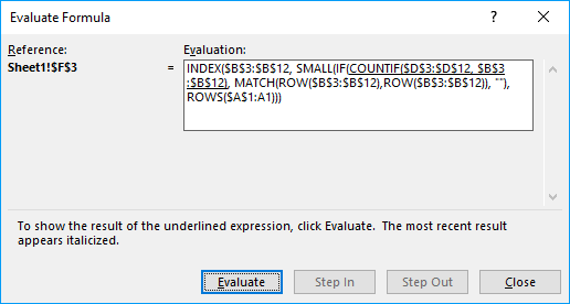
9. Filter common values between two ranges - Excel 2019
Array formula in B12:
Explaining formula in cell B12
Step 1 - Identify values shared by both cell ranges
The COUNTIF function counts values based on a condition or criteria, in this case, it compares values between the cell ranges.
COUNTIF($B$6:$E$9, $B$2:$D$4)>0
becomes
COUNTIF({"HH", "II", "JJ", "KK";"AA", "MM", "NN", "OO";"AA", "QQ", "RR", "SS";"TT", "II", "VV", "CC"}, {"AA", "BB", "CC";"DD", "BB", "EE";"FF", "CC", "GG"})>0
becomes
{2,0,1;0,0,0;0,1,0}>0
and returns
{TRUE, FALSE, TRUE;FALSE, FALSE, FALSE;FALSE, TRUE, FALSE}
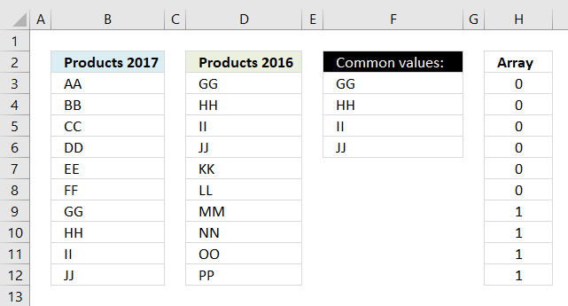
Step 2 - Prevent duplicates
The next COUNTIF function counts values based on a condition or criteria, in this case, we take into account previously displayed values in order to prevent duplicates from showing up in our list.
The first argument in the COUNTIF function B$11:$B11 expands as the cell is copied to cells below, this makes the formula aware of values above the current cell.
COUNTIF($B$11:B11,$B$2:$D$4)=1
becomes
COUNTIF("Common values in range One and Two", {"AA", "BB", "CC";"DD", "BB", "EE";"FF", "CC", "GG"})=1
becomes
{0,0,0;0,0,0;0,0,0}=1
and returns
{FALSE, FALSE, FALSE;FALSE, FALSE, FALSE;FALSE, FALSE, FALSE}.
Step 3 - Add arrays
If at least one of the COUNTIF functions return TRUE then the array returns TRUE or the equivalent value 1.
(COUNTIF($B$6:$E$9,$B$2:$D$4)>0)+COUNTIF(B11:$B$11,$B$2:$D$4))=1
becomes
({TRUE, FALSE, TRUE;FALSE, FALSE, FALSE;FALSE, TRUE, FALSE}+{FALSE, FALSE, FALSE;FALSE, FALSE, FALSE;FALSE, FALSE, FALSE})=1
becomes
{1,0,1;0,0,0;0,1,0}=1
and returns
{TRUE, FALSE, TRUE;FALSE, FALSE, FALSE;FALSE, TRUE, FALSE}.
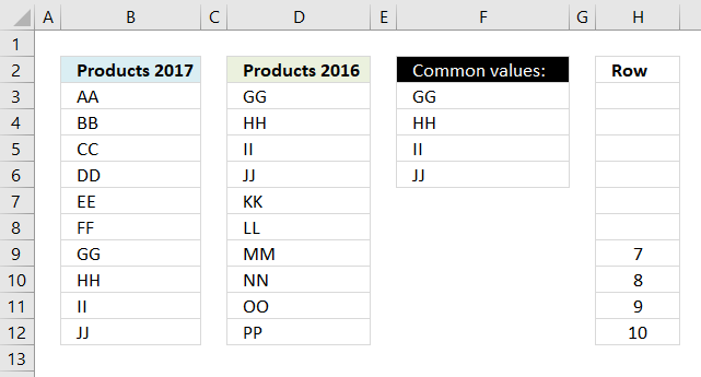
Step 4 - Replace TRUE with coordinates
The following IF function returns the corresponding coordinate if boolean value is TRUE. FALSE returns "" (nothing).
IF(((COUNTIF($B$6:$E$9,$B$2:$D$4)>0)+COUNTIF(B11:$B$11,$B$2:$D$4))=1,(ROW($B$2:$D$4)+(1/(COLUMN($B$2:$D$4)+1)))*1,"")
becomes
IF({TRUE, FALSE, TRUE;FALSE, FALSE, FALSE;FALSE, TRUE, FALSE},(ROW($B$2:$D$4)+(1/(COLUMN($B$2:$D$4)+1)))*1,"")
The ROW and COLUMN functions return the row(s) and column(s) of a cell range. Adding these two numbers creates a unique number for each cell in the cell range.
IF({TRUE, FALSE, TRUE;FALSE, FALSE, FALSE;FALSE, TRUE, FALSE},(ROW($B$2:$D$4)+(1/(COLUMN($B$2:$D$4)+1)))*1,"")
becomes
IF({TRUE, FALSE, TRUE;FALSE, FALSE, FALSE;FALSE, TRUE, FALSE},{2.33333333333333, 2.25, 2.2;3.33333333333333, 3.25, 3.2;4.33333333333333, 4.25, 4.2},"")
and returns
{2.33333333333333,"",2.2;"","","";"",4.25,""}
Step 5 - Get the smallest value in array
The MIN function returns the smallest number in array ignoring blanks and text values.
MIN(IF(((COUNTIF($B$6:$E$9,$B$2:$D$4)>0)+COUNTIF(B11:$B$11,$B$2:$D$4))=1,(ROW($B$2:$D$4)+(1/(COLUMN($B$2:$D$4)+1)))*1,""))
becomes
MIN({2.33333333333333,"",2.2;"","","";"",4.25,""})
and returns 2.2.
Step 6 - Identify value in cell range
IF(MIN(IF(((COUNTIF($B$6:$E$9, $B$2:$D$4)>0)+COUNTIF(B11:$B$11, $B$2:$D$4))=1, (ROW($B$2:$D$4)+(1/(COLUMN($B$2:$D$4)+1)))*1, ""))=(ROW($B$2:$D$4)+(1/(COLUMN($B$2:$D$4)+1)))*1, $B$2:$D$4, "")
becomes
IF(2.2=(ROW($B$2:$D$4)+(1/(COLUMN($B$2:$D$4)+1)))*1,$B$2:$D$4,"")
becomes
IF(2.2={2.33333333333333, 2.25, 2.2; 3.33333333333333, 3.25, 3.2; 4.33333333333333, 4.25, 4.2},$B$2:$D$4,"")
becomes
IF({FALSE,FALSE, TRUE;FALSE, FALSE,FALSE; FALSE,FALSE, FALSE},$B$2:$D$4,"")
and returns
{"","","CC";"","","";"","",""}.
Step 7 - Join text strings in array
The TEXTJOIN function returns values concatenated ignoring blanks in array.
TEXTJOIN("", TRUE, IF(MIN(IF(((COUNTIF($B$6:$E$9, $B$2:$D$4)>0)+COUNTIF(B11:$B$11, $B$2:$D$4))=1, (ROW($B$2:$D$4)+(1/(COLUMN($B$2:$D$4)+1)))*1, ""))=(ROW($B$2:$D$4)+(1/(COLUMN($B$2:$D$4)+1)))*1, $B$2:$D$4, ""))
becomes
TEXTJOIN("", TRUE, {"","","CC";"","","";"","",""})
and returns "CC" in cell B12.
10. Filter common values between two ranges
If your Excel version is missing the TEXTJOIN function then use the following array formula.
Array formula in B12:
To enter an array formula, type the formula in a cell then press and hold CTRL + SHIFT simultaneously, now press Enter once. Release all keys.
The formula bar now shows the formula with a beginning and ending curly bracket telling you that you entered the formula successfully. Don't enter the curly brackets yourself.
Get Excel *.xlsx file
Filter common values from two ranges.xlsx
Filter common values from two rangesv2.xlsx
11. Filter values in common between two cell ranges - UDF
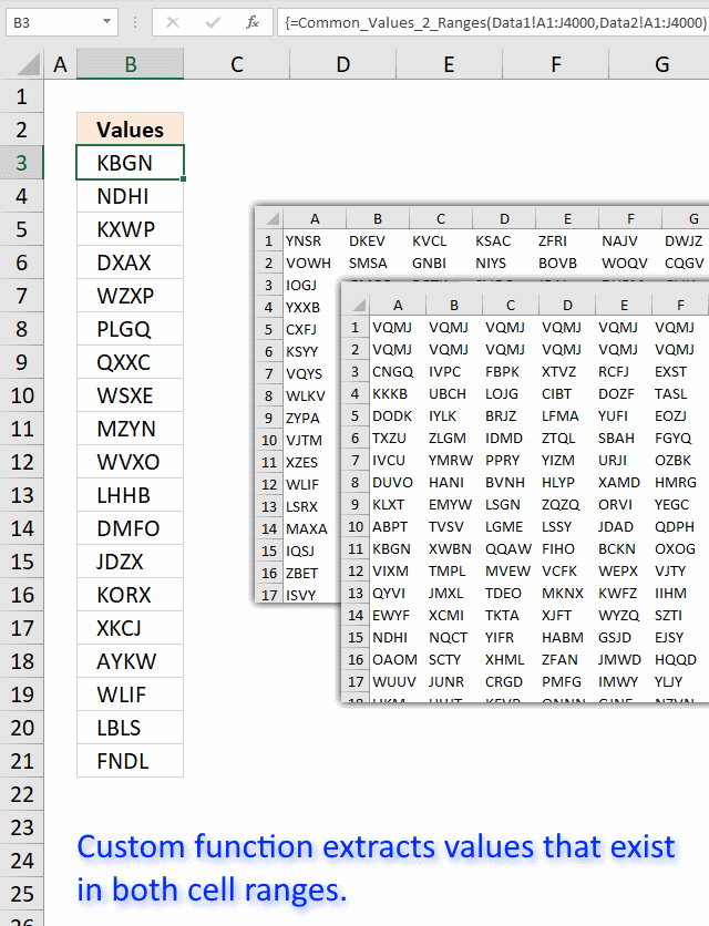
I tried the array formula in this post: Filter common values between two ranges using array formula in excel to extract common values between two cell ranges. 40000 random cell values in each cell range.
As you might have guessed, the array formula is too slow. Sheet2 contains 40000 random text strings in cell range A1:J4000, sheet3 also contains 40000 random text strings in cell range A1:J4000
This udf creates a list of common cell values between the two cell ranges:
User defined function
Function Common_Values_2_Ranges(rng1 As Variant, rng2 As Variant) As Variant

Dim Value1 As Variant
Dim Value2 As Variant
Dim temp() As Variant
Dim Test As New Collection

ReDim temp(0)

rng1 = rng1.Value
rng2 = rng2.Value

On Error Resume Next
For Each Value1 In rng1
 If Len(Value1) > 0 Then Test.Add Value1, CStr(Value1)
Next Value1
On Error GoTo 0

On Error Resume Next
For Each Value2 In rng2
 If Len(Value2) > 0 Then Test.Add Value2, CStr(Value2)
  If Err Then
   temp(UBound(temp)) = Value2
   ReDim Preserve temp(UBound(temp) + 1)
  End If
  Err = False
  Test.Remove Value2
Next Value2
On Error GoTo 0

Common_Values_2_Ranges = Application.Transpose(temp)

End Function
How to add the user defined function to your workbook
- Press Alt-F11 to open visual basic editor
- Press with left mouse button on Module on the Insert menu
- Copy and paste the above user defined function
- Exit visual basic editor
- Select sheet1
- Select cell range A1:A5000
- Type =Common_Values_2_ranges(Sheet2!A1:J4000, Sheet3!A1:J4000) into formula bar and press CTRL+SHIFT+ENTER
- Make sure you save your workbook with the file extension *.xlsm so you can use the UDF the next time you open the same workbook.

Recommended blog post:
Compare two lists of data: Filter common row records in excel
Table category
This article demonstrates different ways to reference an Excel defined Table in a drop-down list and Conditional Formatting formulas. The […]
This article demonstrates two formulas that extract distinct values from a filtered Excel Table, one formula for Excel 365 subscribers […]
The image above demonstrates a macro linked to a button. Press with left mouse button on the button and the […]
How to use Excel Tables
36 Responses to “How to compare two data sets”
Leave a Reply
How to comment
How to add a formula to your comment
<code>Insert your formula here.</code>
Convert less than and larger than signs
Use html character entities instead of less than and larger than signs.
< becomes < and > becomes >
How to add VBA code to your comment
[vb 1="vbnet" language=","]
Put your VBA code here.
[/vb]
How to add a picture to your comment:
Upload picture to postimage.org or imgur
Paste image link to your comment.
If you need to expand your comparison you will need to highlight all the rows, in the column, where you want the common values stored. Paste the above equation into the formula box, may need to use F2 button, and change the values of 17 to however many rows you need. The "" portion of the equation will need retyped as "". Use CTRL + SHFT + ENTER to run comparison. This is due to the equation using an array. Good Luck
Thank you for your comment. I have edited the article.
Oscar,
As usual, another great article. Just wanted to say thanks for all the awesome articles you publish. I always learn something from your work--it is appreciated.
Michael Pennington,
Thank you for commenting!!
hi oscar,
i have a small problem which is similar to the one you have illustrated above, with the only difference being that i have some duplicates within List1 and List2 themselves.
eg. GG is repeated twice in List1, HH is repeated thrice in List2.
when i use this formula, i get duplicate GG and HH in Column 3. is there a way to prevent them from appearing? i tried a mishmash of this formula and a couple of others that i learnt on your website (ones listed in Duplicate category), but to no avail.
please help me out; i will appreciate that very much.
much thanks and kind regards.
K. Yantri,
Use this array formula in cell C2:
hi oscar,
thank you for your kind help in this regard.
Hello,
I am not certain why the range of $A$13:A13 is used in the countif function... Is this a mistake?
Also, how can I adjust this to check for common values in 15 columns? Is that even possible?
Thanks,
Beth
Beth,
I am not certain why the range of $A$13:A13 is used in the countif function... Is this a mistake?
It makes sure that only unique distinct values are extracted.
See the explanation in this post:
Filter values that exists in all three lists
Also, how can I adjust this to check for common values in 15 columns? Is that even possible?
Yes, add the remaining 12 columns to the formula, using a countif function for each column. See explanation.
Absolutely outstanding! I struggled with a solution for weeks. Thank you not only for the solution but the explanation of how it all works.
I am not able to do this for some reason... Using Excel 2011 on a Mac.
"Formula refers to empty cells." error...
Vanessa,
Try creating tables instead of dynamic named ranges.
Try creating tables instead of dynamic named ranges.
i love it
Hi,
I am trying to compare the values in the excel where i have got list of values in the Column A and List of Values in Column B.
I want to find all the duplicate values in Row 1 and Row 2 but when i am applying above formulas getting #Value! error.
Anoop,
How to create an array formula
1.Select cell C2
2.Press with left mouse button on formula bar
3.Copy Paste array formula
4.Press and hold Ctrl + Shift
5.Press Enter
Hi Oscar,
Thanks for your quick reply.
PSB the proper example of my prob:-
Question 1 How can we identify duplicate values from each column?
Question 2 If it is not possible to compare 4 column can we do it for 2?
Data 1 Data 2 Data 3 Data 4
1 5 9 11
2 6 10 12
3 4 4 4
4 7 7 7
5 8 8 8
Multi-nested formulas, as the one above, can be tough to decipher
The free/unlocked function syntax and usage navigation Add-in (link below) can speed-up your modelling work, if you are:
1) looking for multi-lingual documentation or translation for a function
2) searching for a new function to simplify your formulas
3) wondering, if a function is backwards compatible with previous Excel versions
https://www.spreadsheet1.com/syntax-and-usage-navigation-add-in-for-excel-2013-functions.html
More complicated if we have 3 columns to compare the duplicates, you have the sample cases or formula for 3 column to retrieve duplicates?
Thanks
Rizky,
The example in this post compares 3 columns. Can you explain in greater detail?
Im sorry not inform clear to you, I mean compare 3 list, and is it possible retrieve common records with criteria? For example I want to retrieve common records between 2 or more list with criteria year 1997?
Hi Oscar,
Is there a way to do what you did above but without the named ranges?
Thanks
Dan
Hi Oscar,
Need a formula to count identical numbers in two columns but items must be in same row (position).
12 15
8 8 good count 1
22 19
7 22 for 22 not count cause is not in same row
14 14 good count 2
....
....
Thanks.
[…] Kidd asks: […]
How can we find common numbers from different sheets and arrange them with column heading and by counting that how many time a found in which Sheet???
[…] { googletag.display('div-gpt-ad-1486744346002-0'); }); Hi have a look at How to find common values from two lists | Get Digital Help - Microsoft Excel resource that should do the […]
I am running your UDF function and not sure what Err does. When you test for If Err, what specific condition are you looking for here?
Ekaterina Boehm
Err checks if there was an error adding the text string to the collection.
It means that the text string is already in the collection so it must be a value found in both cell ranges.
REGARDING THE ABOVE QUESTION "Also, how can I adjust this to check for common values in 15 columns? Is that even possible?
Yes, add the remaining 12 columns to the formula, using a countif function for each column. See explanation."
Can you tell me what to insert - for my 3 columns I have =INDEX(A2:A16, MATCH(0, COUNTIF($A$19:A19, A2:A16)+IF(IF(COUNTIF(B2:B16, A2:A16)>0, 1, 0)+IF(COUNTIF(C2:C16, A2:A16)>0, 1, 0)=2, 0, 1), 0)). How do I add further columns into the range? I have tried copy and pasting +IF(COUNTIF(C2:C16, A2:A16)>0, 1, 0)before the = and changing it to d2:d16 but get an error
Louise
Great question!
Array formula in cell B14:
To add a fifth column (Col E) simply add a COUNTIF function.
I tried below formula for the fourth and fifth columns but only one item is listed other NA
What did I do wrong??
Array formula in cell B14:
=INDEX($A$2:$A$11,MATCH(0, COUNTIF($B$13:B13, $A$2:$A$11)+NOT(COUNTIF($B$2:$B$10, $A$2:$A$11)*COUNTIF($C$2:$C$11, $A$2:$A$11)*COUNTIF($D$2:$D$9, $A$2:$A$11)), 0))
To add a fifth column (Col E) simply add a COUNTIF function.
=INDEX($A$2:$A$11,MATCH(0, COUNTIF($B$13:B13, $A$2:$A$11)+NOT(COUNTIF($B$2:$B$10, $A$2:$A$11)*COUNTIF($C$2:$C$11, $A$2:$A$11)*COUNTIF($D$2:$D$9, $A$2:$A$11)*COUNTIF($E$2:$E$9, $A$2:$A$11)), 0))
Albert,
Can you post your formula?
Hi Oscar! I liked your solution. It worked fine for me.
However I have a different challenge now: to make it work for 7 columns, where I may select only some of them to make this analysis. The way the formula is will only return me a value which is common for all the 7columns. Id like to have the chance to select 2 or 3 columns for instance (out of those 7) to apply the search. Of course the selected ones may change on each use. Any idea? Thank you much!
Thanks for such a good explanation.
Hi there! This is a great formula, how can I make sure it is case sensitive? Appreciate any info you can provide. Thanks
Jjoseph,
thank you! I have added a case sensitive formula to this article.