How to use the GROUPBY function
What is the GROUPBY function?
The GROUPBY function allows you to aggregate data through a formula vertically. It is a formula-based alternative to the traditional pivot table for many summarizing operations. The function is a dynamic array formula and is only available to Excel 365 subscribers.
Table of Contents
- Introduction
- Syntax
- Example 1 - create totals by category
- Example 2 - aggregate by category and sort from large to small
- Example 3 - summarize by two categories
- Example 4 - create totals by year
- Example 5 - aggregate by year and month
- Example 6 - summarize by year and quarter
- Example 7 - create totals by year and week
- Example 8 - create totals and count in the same column
- Example 9 - aggregate values and sort by count
- Example 10 - aggregate values and display corresponding invoice numbers
- Extract unique distinct values sorted based on sum of adjacent values - Excel 365
- Extract unique distinct values sorted based on sum of adjacent values - earlier Excel versions
- Filtering unique distinct text values and sorting them based on the sum of adjacent values and criteria - earlier Excel versions
- Filtering unique distinct text values and sorting them based on the sum of adjacent values and criteria - Excel 365
1. Introduction
What is a dynamic array formula?
A dynamic array formula in Excel 365 is a type of formula that can return multiple values which are then automatically spills into a range of adjacent cells below and/or to the right. This allows for more flexible and dynamic calculations as the formula can adapt to the size of the data. Dynamic array formulas in Excel 365 are entered as regular formulas in contrast to array formulas in older Excel versions that required you to press CTRL + SHIFT + ENTER.
What is spilling?
Spilling in Excel 365 refers to the process of a formula returning multiple values, which are then automatically displayed in a range of cells. This is a key feature of dynamic array formulas, as it allows the formula to adapt to the size of the data and display the results in a flexible and dynamic way. When a formula spills, the values are displayed in a range of cells, and the formula is denoted by a blue border.
What is aggregating values?
Aggregating values in Excel refers to the process of combining multiple values into a single value often using a mathematical operation such as sum, average, or count. Aggregating values is a common task in data analysis, as it allows you to summarize and analyze large datasets.
What is a pivot table?
A pivot table in Excel is a powerful data analysis tool that allows you to summarize and analyze large datasets.
- A pivot table is a table that can be rotated and manipulated to display different views of the data allowing you to easily summarize and analyze the data from different angles.
- Pivot tables are particularly useful for analyzing large datasets as they allow you to quickly and easily summarize and analyze the data, and to create custom views of the data.
- Pivot tables can be used to perform a variety of tasks, including aggregating values, filtering data, and creating custom reports.
The GROUPBY function allows for aggregating values in rows or vertically. How can I aggregate values also in columns or horizontally?
The PIVOTBY function allows for summarizing for both rows (vertically) and columns (horizontally).
What are the benefits of using the GROUPBY function instead of using a Pivot Table?
- You can analyze text values as well. This is not possible with the Pivot Table.
- Changes in the source data is immediately shown in the formula output. This is not the case with Pivot Tables, you need to refresh the Pivot Table in order to calculate new aggregated values.
2. Syntax
GROUPBY(row_fields, values, function, [field_headers], [total_depth], [sort_order], [filter_array], [field_relationship])
| Argument | Text |
| row_fields | Required. The fields that determines the aggregated values. You may use multiple fields. |
| values | Required. The data you want to aggregate. |
| function | Required. The function that is used to aggregate values.
SUM: The sum of a range of cells. |
| [field_headers] | Optional. A number between 0 (zero) and 3, if missing automatic mode which is the default. Automatic determines if the data source contains headers based on their data type text or number. Missing: Automatic. (default) 0: No 1: Yes and don't show 2: No but generate 3: Yes and show |
| [total_depth] | Optional. This specifies if the row headers should disply totals.
Missing: Automatic: Grand totals and, where possible, subtotals. (default) |
| [sort_order] | Optional. A number that corresponds to the columns in the row_fields argument. A positive number and the rows are sorted in ascending order, a negative numbers sorts the rows in descending order. |
| [filter_array] | Optional. A logical expression that evaluates to TRUE or FALSE which indicates if the corresponding value is included in the calculation. |
| [field_relationship] | Optional. A number:
0: Hierarchy (defualt) sorting takes into account the hierarchy of earlier columns. 1: Sorting is done independently. Subtotals are not supported. |
3. Example 1 - aggregate based on item
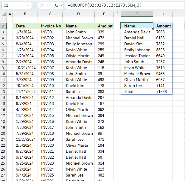
This example demonstrates how to aggregate values based on items, in this case, names. The output array contains header names. The image above shows an Excel spreadsheet containing invoice numbers (source data) and a summary table. The main table (columns A-E) has the following columns: Date, Invoice No, Name, Amount. It lists various transactions with dates ranging from 2024, invoice numbers (INV001-INV031), customer names, and corresponding amounts.
The formula shown in the formula bar is the contents of cell G2:
The arguments are:
- row_fields - D2:D273 The column header name is included in the cell reference.
- values - E2:E273 The column header name is included in the cell reference.
- function - SUM
- [field_headers] - 3 representing "Yes, and show".
To the right (columns F-G) is a summary table that is generated using a GROUPBY function. This table shows:"Name" and "Amount" The Amount column in the summary table is the total amount for each unique name from the main table. At the bottom of this summary, there's a "Total" row showing the total of all aggregated amounts.
This summary is created by grouping the data from the main table by name and aggregating the amounts for each person. This spreadsheet tracks financial transactions or sales by individual with the summary providing a quick overview of total amounts per person.
4. Example 2 - aggregate based on item and sort
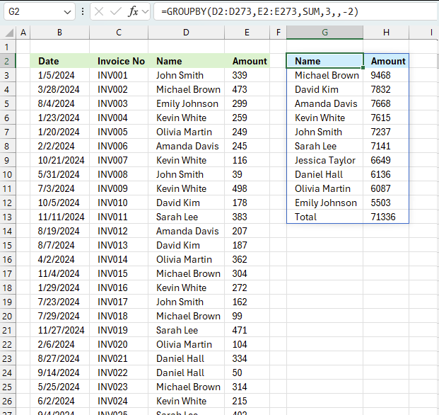
This example shows how to summarize sales amounts based on names, the output is sorted based on output column in descending order meaning from large to small.
The source data is in cell range B3:E273, it contains 4 columns with header names Date, Invoice No, Name, and the corresponding amount.
The formula shown in the formula bar is the contents of cell G2:
The arguments are:
- row_fields - D2:D273 The column header name is included in the cell reference.
- values - E2:E273 The column header name is included in the cell reference.
- function - SUM
- [field_headers] - 3 representing "Yes, and show".
- [sort_order] - -2 meaning the output array is sorted based on column 2 in descending order.
The image above shows the output array in cell range G2:H13.
5. Example 3 - aggregate based on two items
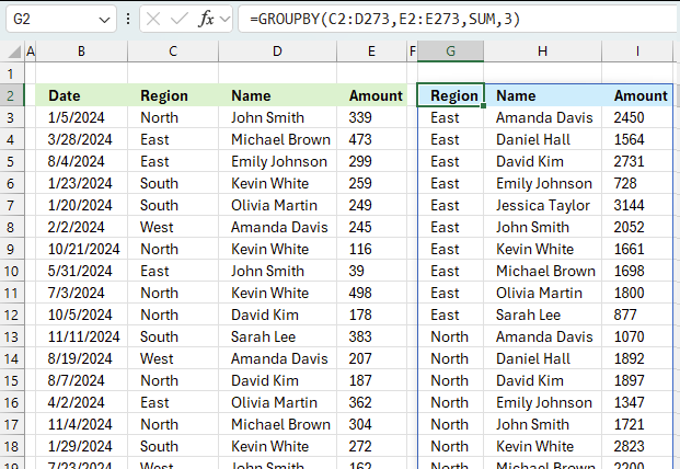
This example shows how to summarize numbers based on two categories, in this case "Region" and "Name". The amounts on the same row corresponds to the "Region" and "Name". The source data is in cell range B3:E273, it contains the following columns: "Date", "Region", "Name", and "Amount".
The arguments are:
- row_fields - D2:D273 The column header name is included in the cell reference.
- values - E2:E273 The column header name is included in the cell reference.
- function - SUM
- [field_headers] - 3 representing "Yes, and show".
Note that the cell references contain the column header names as well. This allows you to show the column names if 3 is specified in the fourth argument named [field_headers] which tells the function to display the included column header names.
The difference between this example and example 1 above is that the first argument contains two columns instead of one. The output array contains both these columns, however, duplicate rows are merged into one distinct row.
6. Example 4 - aggregate based on year
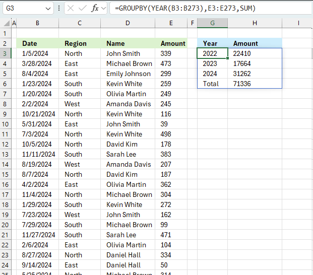
The image above shows the function in cell G3. the column header names above are hard coded meaning they are actual typed values and not the result of a formula. The source data is in cell range B3:E273, it contains the following columns: "Date", "Region", "Name", and "Amount".
The arguments are:
- row_fields - YEAR(B3:B273) The column header name is not included in the cell reference.
- The YEAR function returns the year based on an Excel date. It has the following syntax: YEAR(serial)
Serial is the actual Excel date or in this case multiple Excel dates.
- The YEAR function returns the year based on an Excel date. It has the following syntax: YEAR(serial)
- values - E3:E273 The column header name is included in the cell reference.
- function - SUM
The output array, displayed in cell G3 and adjacent cells below and to the right, summarizes the amounts based on the corresponding year based on the specified date in column "Date".
- YEAR(B3:B273): This part extracts the year from dates in the range B3:B273. It creates a array of years, which will be used as the grouping criteria.
- E3:E273: This is the range of values to be summarized which is the "Amount" column in the data set.
- SUM: This is the operation to be performed on the grouped data.
What this formula does:
- It groups the data by year (extracted from column B).
- For each unique year, it sums the corresponding values from column E.
The result will be a summary table showing:
- Unique years from column B
- Total sum of amounts (from column E) for each year
This formula is useful for creating an annual summary of financial data, showing the total amount for each year represented in the dataset.
7. Example 5 - aggregate based on year and month

This example demonstrated in the image above shows the function in cell G3. the column header names above are hard coded meaning they are actual typed values and not the result of a formula. The source data is in cell range B3:E273, it contains the following columns: "Date", "Region", "Name", and "Amount".
The arguments are:
- row_fields - TEXT(B3:B273,"yyyy-mmm") The column header name is not included in the cell reference.
- The TEXT function returns the year and month based on an Excel date in column B. It has the following syntax: TEXT(value, format_code)
Value is the actual Excel date or in this case multiple Excel dates.
- The TEXT function returns the year and month based on an Excel date in column B. It has the following syntax: TEXT(value, format_code)
- values - E3:E273 The column header name is included in the cell reference.
- function - SUM
The output array, displayed in cell G3 and adjacent cells below and to the right, summarizes the amounts based on the corresponding year and month based on the specified date in column "Date".
- TEXT(B3:B273,"yyyy-mmm") : This part extracts the year and month from dates in the range B3:B273. It creates a array of years and months, which will be used as the grouping criteria.
- E3:E273: This is the range of values to be summarized which is the "Amount" column in the data set.
- SUM: This is the operation to be performed on the grouped data.
What this formula does:
- It groups the data by year and month extracted from column B.
- For each unique year and month, it sums the corresponding values from column E.
The result will be a summary table showing:
- Unique years and months from column B
- Total sum of amounts (from column E) for each year
This formula is useful for creating an monthly summary of financial data, showing the total amount for each month represented in the dataset.
8. Example 6 - aggregate values based on year and quarter
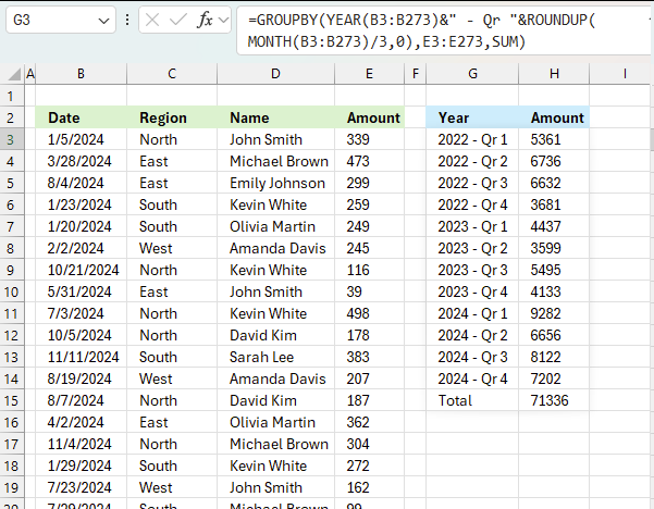
This example demonstrates how to aggregate values based on year and quarter using the GROUPBY function in cell G3. The column header names above are hard coded meaning they are actual typed values and not the result of a formula. The source data is in cell range B3:E273, it contains the following columns: "Date", "Region", "Name", and "Amount".
The arguments are:
- row_fields - YEAR(B3:B273)&" - Qr "&ROUNDUP(MONTH(B3:B273)/3,0) The column header name is not included in the cell reference.
- The YEAR function returns the year based on an Excel date in column B. It has the following syntax: YEAR(serial).
- The ampersand character & concatenates values.
- ROUNDUP(MONTH(B3:B273)/3,0) calculates the quarter number.
- values - E3:E273 The column header name is included in the cell reference.
- function - SUM
The output array, displayed in cell G3 and adjacent cells below and to the right, summarizes the amounts based on the corresponding year and quarter calculated based on the specified date in column "Date".
- YEAR(B3:B273): Extracts the year from the dates in the range B3:B273.
- MONTH(B3:B273): Extracts the month number (1-12) from the dates in the range B3:B273.
- MONTH(B3:B273)/3 Divides the month number by 3.
- ROUNDUP(..., 0): Rounds up the result of the division to the nearest integer, effectively giving us the quarter number. This gives a decimal value representing the quarter:
- Months 1-3 (Q1): result 1
- Months 4-6 (Q2): result 2
- Months 7-9 (Q3): result 3
- Months 10-12 (Q4): result 4
- " - Qr ":A literal string that will separate the year from the quarter in the final output.
- &: The ampersands concatenate all these parts into a single string.
The complete formula YEAR(B3:B273)&" - Qr "&ROUNDUP(MONTH(B3:B273)/3,0) will produce results like:
"2024 - Qr 1" for dates in January, February, or March 2024
"2024 - Qr 2" for dates in April, May, or June 2024
"2024 - Qr 3" for dates in July, August, or September 2024
"2024 - Qr 4" for dates in October, November, or December 2024
This formula is useful for grouping dates by both year and quarter, which can be helpful for financial reporting or seasonal analysis of data.
What this formula does:
- It groups the data by year and quarter extracted from column B.
- For each unique year and quarter, it sums the corresponding values from column E.
The result will be a summary table showing:
- Unique years and quarters from column B
- Total sum of amounts (from column E) for each year
This formula is useful for creating an quarterly summary of financial data, showing the total amount for each quarter represented in the dataset.
9. Example 7 - aggregate values based on year and week

This example demonstrates how to aggregate values based on year and week number using the GROUPBY function in cell G3. The column header names above are hard coded meaning they are actual typed values and not the result of a formula. The source data is in cell range B3:E273, it contains the following columns: "Date", "Region", "Name", and "Amount".
Formula in cell G3:
The arguments are:
- row_fields - HSTACK(YEAR(B3:B273),BYROW(B3:B273,LAMBDA(a,WEEKNUM(a,1)))) The column header name is not included in the cell reference.
- values - G3:G273 The column header name is not included in the cell reference.
- function - SUM
The output array is shown in cell I3 and adjacent cells to the right and below. It displays aggregated amounts based on year and week number specified in column B and C.
Here is a quick break down of the formula:
- HSTACK: This function horizontally combines arrays or values.
Inside HSTACK, we have two arguments:- YEAR(B3:B273):
- This extracts the year from each date in the range B3:B273.
- It creates a single-column array of years.
- The WEEKNUM function does not allow an array of values, we need a workaround. The BYROW function lets us use a cell range as an input value.
BYROW(B3:B273,LAMBDA(a,WEEKNUM(a,1))):- BYROW applies a function to each row of the given range.
- The LAMBDA function defines what to do for each row:
WEEKNUM(a,1) calculates the week number of the date in each row.
The ",1" in WEEKNUM meaning week begins on Sunday.
- YEAR(B3:B273):
- GROUPBY(HSTACK(...),E3:E273,SUM): This aggregates values in E3:E273 based on the given year and week numbers
10. Example 8 - aggregate values and display sum and count
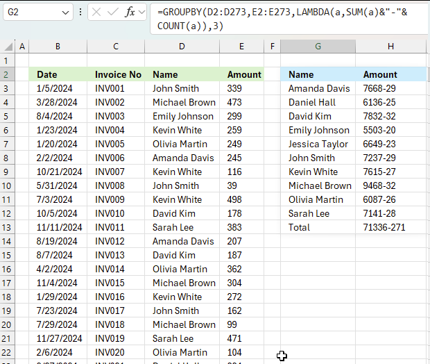
This example shows how to aggregate numbers and show the corresponding count meaning how many values are included in each summary. The down side is that you want be able to sort the values since they now are text values. The first value shown in cell G3 is "Amanda Davis", the sum is 7668 shown in cell H3 and after the hyphen "-" the total number of indivdual numbers in sum sum are shown. In this case, 29 numbers are included in the sum of 7668.
The formula in cell G2:
This formula uses the GROUPBY function in Excel along with a LAMBDA function to create a custom summary. Let's break it down:
- D2:D273 - This is the first argument of GROUPBY and represents the column to group by, likely the "Name" column in your data.
- E2:E273 - This is the second argument, representing the values to summarize, likely the "Amount" column.
- LAMBDA(a,SUM(a)&"-"&COUNT(a)) - This is a custom aggregation function:
- LAMBDA(a, ...) defines an anonymous function where 'a' represents each group of values.
- SUM(a) calculates the total sum for each group.
- COUNT(a) counts the number of items in each group.
- & "-" & concatenates the sum and count with a hyphen between them.
- 3: This argument specifies that header names will be shown.
The result of this formula will be a summary table with:
- Column 1: Unique names from column D
- Column 2: A string in the format "Sum-Count" for each name, where:
- Sum is the total amount for that name
- Count is the number of entries for that name
For example, if John Smith had 3 invoices totaling $1000, his row in the summary might look like: John Smith | 1000-3 |
This formula provides a concise summary of both the total amount and the number of transactions for each unique name in your dataset.
11. Example 9 - aggregate values and sort by count
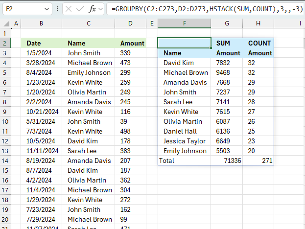
Example 8 above showed how to display both the sum and the count for each category, however, this made it hard to sort the values as both values concatenated in the same cell creates a text string. This example shows how to build a formula that creates both the amount and the count in different columns which enables sorting based on the count.
Formula in cell F3:
The arguments are:
- row_fields - C2:C273 The column header name is included in the cell reference.
- values - C2:C273 The column header name is included in the cell reference.
- function - HSTACK(SUM,COUNT) - The HSTACK function allows for multiple functions, all in different columns. This example demonstrates SUM and COUNT functions.
- [field_headers] - 3 representing "Yes, and show".
- [sort_order] - -3 meaning sort on the third column (COUNT) from large to small
12. Example 10 - aggregate values and display corresponding invoice numbers
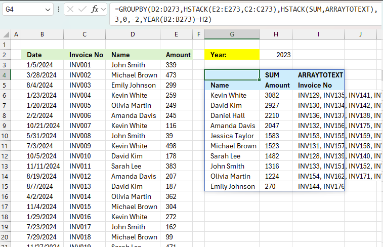
This example shows how to:
- filter values using the [filter_array] argument based on year specified in yellow cell H2
- aggregate amounts based on names in column H
- sort the totals in descending order meaning from large to small
- display corresponding invoice numbers horizontally in columns I and adjacent columns to the right
all in one formula
Excel 365 dynamic array formula in cell G4:
The arguments in the GROUPBY function are:
- row_fields - D2:D273 The column header name is included in the cell reference.
- values - HSTACK(E2:E273,C2:C273) The column header name is included in the cell reference. The HSTACK function allows for multiple columns, in this case, both the values and invoice numbers.
- function - HSTACK(SUM,ARRAYTOTEXT): The HSTACK function allows for multiple functions as well, in this case, both aggregate and text values.
- 3 - show column header names
- 0 - no grand total
- -2 - sort values based on column 2 (aggregated numbers) from large to small
- YEAR(B2:B273)=H2 - filter values if date in column B is in the same year as specified in cell H2
13. Extract unique distinct values sorted based on sum of adjacent values - Excel 365

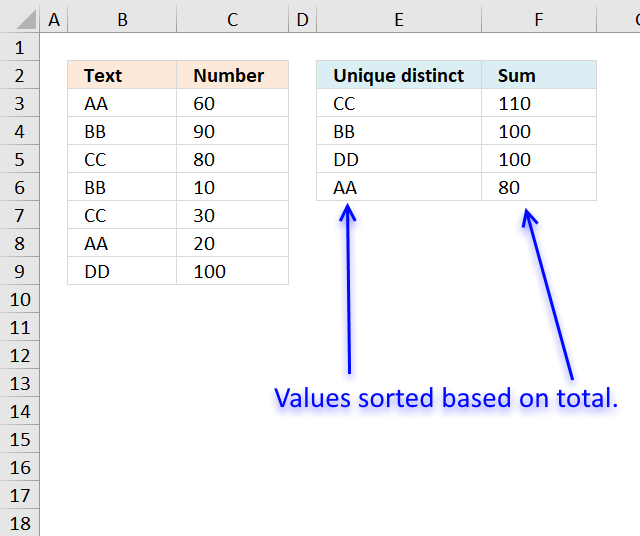
This example demonstrates a formula that lists unique distinct values in column B and returns a sorted list based on the totals in column C from large to small.
Value "CC" is displayed in cells C5 and C7, they are 80 and 30 respectively, and the total is 110.
Value "BB" is displayed in cells C4 and C6, they are 90 and 10 respectively, and the total is 100.
Value "DD" is displayed in cell C9, the value is 100, and the total is 100.
Value "AA" is displayed in cells C3 and C7, they are 60 and 20 respectively, and the total is 80.
Update! New function in Excel 365!
Excel 365 dynamic array formula in cell E3:
Read more about the GROUPBY function.
Excel 365 dynamic array formula:
Formula in cell F3:
Explaining formula
Step 1 - Extract unique distinct values
The UNIQUE function returns a unique or unique distinct list.
Function syntax: UNIQUE(array,[by_col],[exactly_once])
UNIQUE(B3:B9)
becomes
UNIQUE({"AA";"BB";"CC";"BB";"CC";"AA";"DD"})
and returns
{"AA";"BB";"CC";"DD"}.
Step 2 - Calculate totals based on the unique list
The SUMIF function sums numerical values based on a condition.
Function syntax: SUMIF(range, criteria, [sum_range])
SUMIF(B3:B9,UNIQUE(B3:B9),C3:C9)
becomes
SUMIF({"AA";"BB";"CC";"BB";"CC";"AA";"DD"}, {"AA";"BB";"CC";"DD"}, {60;90;80;10;30;20;100})
and returns
{80;100;110;100}
Step 3 - Sort totals from largest to smallest
The SORTBY function sorts a cell range or array based on values in a corresponding range or array.
Function syntax: SORTBY(array, by_array1, [sort_order1], [by_array2, sort_order2],…)
SORTBY(UNIQUE(B3:B9),SUMIF(B3:B9,UNIQUE(B3:B9),C3:C9),-1)
becomes
SORTBY({"AA";"BB";"CC";"DD"},{60;90;80;10;30;20;100},-1)
and returns
{"CC";"BB";"DD";"AA"}.
Step 4 - Shorten the formula
The LET function lets you name intermediate calculation results which can shorten formulas considerably and improve performance.
Function syntax: LET(name1, name_value1, calculation_or_name2, [name_value2, calculation_or_name3...])
SORTBY(UNIQUE(B3:B9),SUMIF(B3:B9,UNIQUE(B3:B9),C3:C9),-1)
y - B3:B9
x - UNIQUE(y)
LET(y,B3:B9,x,UNIQUE(y),SORTBY(x,SUMIF(y,x,C3:C9),-1))
14. Extract unique distinct values sorted based on the sum of adjacent values - earlier Excel versions
This formula is for earlier Excel versions.
Array formula in E2:
How to create an array formula
- Copy above array formula
- Double press with left mouse button on cell E3
- Paste array formula
- Press and hold Ctrl + Shift simultaneously
- Press Enter
Formula in cell F3:
Explaining formula in cell E2
Step 1 - Count prior values above the current cell
The COUNTIF function counts values based on a condition or criteria, if the number is 0 (zero) then the corresponding value has not yet been displayed.
NOT(COUNTIF($D$1:D1, $A$2:$A$8))
becomes
NOT(COUNTIF("Unique distinct", {"AA";"BB";"CC";"BB";"CC";"AA";"DD"}))
becomes
NOT({0;0;0;0;0;0;0})
The NOT function returns the boolean opposite to the given argument. The array contains no boolean values, however it does contain their numerical equivavents. TRUE = 1 and FALSE = 0 (zero).
NOT({0;0;0;0;0;0;0})
and returns
{TRUE; TRUE; TRUE; TRUE; TRUE; TRUE; TRUE}.
Step 2 - IF TRUE then return the corresponding sum
The IF function returns the total if the boolean value is TRUE. FALSE returns "" (nothing).
IF(NOT(COUNTIF($E$2:E2, $B$3:$B$9)),SUMIF($B$3:$B$9, "="&$B$3:$B$9, $C$3:$C$9),"")
becomes
IF({TRUE; TRUE; TRUE; TRUE; TRUE; TRUE; TRUE}, SUMIF($B$3:$B$9, "="&$B$3:$B$9, $C$3:$C$9),"")
The SUMIF function adds numbers and returns a total based on a condition or criteria.
IF({TRUE; TRUE; TRUE; TRUE; TRUE; TRUE; TRUE}, SUMIF($B$3:$B$9, "="&$B$3:$B$9, $C$3:$C$9),"")
becomes
IF({TRUE; TRUE; TRUE; TRUE; TRUE; TRUE; TRUE}, {80;100;110;100;110;80;100},"")
and returns
{80;100;110;100;110;80;100}.
Step 3 - Get the largest number in array
The MAX function returns the largest number in the array ignoring blanks and text values.
MAX(IF(NOT(COUNTIF($E$2:E2, $B$3:$B$9)),SUMIF($B$3:$B$9, "="&$B$3:$B$9, $C$3:$C$9),""))
becomes
MAX({80;100;110;100;110;80;100})
and returns 110.
Step 4 - Match number
The MATCH function returns the relative position of a value in a cell range or array.
MATCH(MAX(IF(NOT(COUNTIF($E$2:E2, $B$3:$B$9)),SUMIF($B$3:$B$9, "="&$B$3:$B$9, $C$3:$C$9),"")), IF(NOT(COUNTIF($E$2:E2, $B$3:$B$9)),SUMIF($B$3:$B$9, "="&$B$3:$B$9, $C$3:$C$9),""), 0)
becomes
MATCH(110, IF(NOT(COUNTIF($E$2:E2, $B$3:$B$9)),SUMIF($B$3:$B$9, "="&$B$3:$B$9, $C$3:$C$9),""), 0)
becomes
MATCH(110, {80;100;110;100;110;80;100}, 0)
and returns 3.
Step 5 - Get value
The INDEX function returns a value based on row number (and column number if needed)
INDEX($A$2:$A$8, MATCH(MAX(IF(NOT(COUNTIF($D$1:D1, $A$2:$A$8)),SUMIF($A$2:$A$8, "="&$A$2:$A$8, $B$2:$B$8),"")), IF(NOT(COUNTIF($D$1:D1, $A$2:$A$8)),SUMIF($A$2:$A$8, "="&$A$2:$A$8, $B$2:$B$8),""), 0))
becomes
INDEX($A$2:$A$8, 3)
and returns "CC" in cell E2.
Get Excel *.xlsx file
Filter unique distinct list sorted based on sum of adjacent values.xlsx
15. Filtering unique distinct text values and sorting them based on the sum of adjacent values and criteria - earlier Excel versions

This formula is for earlier Excel versions than Excel 365. It extracts values based on the list specified in cells E1 and E2, the formula returns the list sorted based on totals of the adjacent numbers.
Array formula in cell E7:
Formula in cell E7:
Get excel *.xlsx file
filter-unique-distinct-list-sorted-based-on-sum-of-adjacent-values-using-array-formula2.xlsx
16. Filtering unique distinct text values and sorting them based on the sum of adjacent values and criteria - Excel 365

This formula is the same as in section 1 with one difference, values must be in the criteria list in order to be displayed.
Update!
The following formula demonstrates the new GROUPBY function, it has the following arguments:
- row_fields - B3:B9 (text values)
- values - C3:C9 (Numbers)
- function - SUM (Calculates totals based on numbers)
- [field_headers] - 0 (zero) - no column headers
- [total_depth]- 0 - no totals
- [sort_order]- -2 - sort based on column 2 in descending order
- [filter_array] - COUNTIF(F2:F3,B3:B9) - Filter values based on criteria specified in cells F2:F3
Excel 365 formula:
Excel 365 dynamic array formula in cell E6:
Formula in cell F6:
Explaining formula
Step 1 - Count values based on criteria
The COUNTIF function calculates the number of cells that is equal to a condition.
Function syntax: COUNTIF(range, criteria)
COUNTIF(F2:F3,B3:B9)
becomes
COUNTIF({"AA";"BB"},{"AA";"BB";"cc";"EE";"cc";"F F";"DD"})
and returns
{1; 1; 0; 0; 0; 0; 0}.
Step 2 - Filter values based on the count
The FILTER function extracts values/rows based on a condition or criteria.
Function syntax: FILTER(array, include, [if_empty])
FILTER(B3:B9,COUNTIF(F2:F3,B3:B9))
becomes
FILTER({"AA";"BB";"cc";"EE";"cc";"F F";"DD"},{1; 1; 0; 0; 0; 0; 0})
and returns
{"AA";"BB"}.
Step 3 - Extract unique distinct values
The UNIQUE function returns a unique or unique distinct list.
Function syntax: UNIQUE(array,[by_col],[exactly_once])
UNIQUE(FILTER(B3:B9,COUNTIF(F2:F3,B3:B9)))
becomes
UNIQUE({"AA";"BB"})
and returns
{"AA";"BB"}.
Step 4 - Calculate totals based on the unique list
The SUMIF function sums numerical values based on a condition.
Function syntax: SUMIF(range, criteria, [sum_range])
SUMIF(B3:B9,UNIQUE(FILTER(B3:B9,COUNTIF(F2:F3,B3:B9))),C3:C9)
becomes
SUMIF({"AA";"BB";"cc";"EE";"cc";"F F";"DD"}, {"AA";"BB"}, {60;90;80;-100;30;-50;0})
and returns
{60;90}.
Step 5 - Sort totals from largest to smallest
The SORTBY function sorts a cell range or array based on values in a corresponding range or array.
Function syntax: SORTBY(array, by_array1, [sort_order1], [by_array2, sort_order2],…)
SORTBY(UNIQUE(FILTER(B3:B9,COUNTIF(F2:F3,B3:B9))),SUMIF(B3:B9,UNIQUE(FILTER(B3:B9,COUNTIF(F2:F3,B3:B9))),C3:C9),-1)
becomes
SORTBY({"AA";"BB"},{60;90},-1)
and returns
{"BB";"AA"}.
Step 6 - Shorten the formula
The LET function lets you name intermediate calculation results which can shorten formulas considerably and improve performance.
Function syntax: LET(name1, name_value1, calculation_or_name2, [name_value2, calculation_or_name3...])
SORTBY(UNIQUE(FILTER(B3:B9,COUNTIF(F2:F3,B3:B9))),SUMIF(B3:B9,UNIQUE(FILTER(B3:B9,COUNTIF(F2:F3,B3:B9))),C3:C9),-1)
y - B3:B9
x - UNIQUE(FILTER(y,COUNTIF(F2:F3,y)))
LET(y,B3:B9,x,UNIQUE(FILTER(y,COUNTIF(F2:F3,y))),SORTBY(x,SUMIF(y,x,C3:C9),-1))
'GROUPBY' function examples
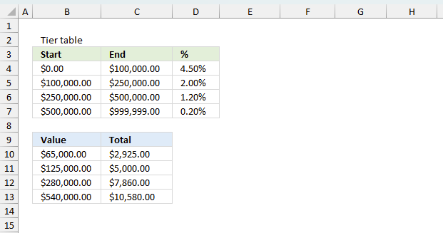
The image above demonstrates a formula that calculates tiered values based on a tier table and returns a total. This […]
Functions in 'Math and trigonometry' category
The GROUPBY function function is one of 62 functions in the 'Math and trigonometry' category.
Excel function categories
Excel categories
13 Responses to “How to use the GROUPBY function”
Leave a Reply
How to comment
How to add a formula to your comment
<code>Insert your formula here.</code>
Convert less than and larger than signs
Use html character entities instead of less than and larger than signs.
< becomes < and > becomes >
How to add VBA code to your comment
[vb 1="vbnet" language=","]
Put your VBA code here.
[/vb]
How to add a picture to your comment:
Upload picture to postimage.org or imgur
Paste image link to your comment.
[...] Filter unique distinct list sorted based on sum of adjacent values … [...]
How might I go about doing this if the values range from positive to negative. ie.
Text Number
AA 60
BB 90
CC 80
EE -100
CC 30
FF -50
DD 100
Eric,
Array formula in A11:
=INDEX(List_text, MATCH(LARGE(IF(COUNTIF($A$10:A10, List_text)=0, SUMIF(List_text, "="&List_text, List_number), ""), 1), SUMIF(List_text, "="&List_text, List_number)*NOT(COUNTIF($A$10:A10, List_text)), 0)) + CTRL + SHIFT + ENTER. Copy cell A11 and paste it down as far as necessary.
Hi Oscar,
Thanks for the formula above, it fixes the case where there are negative values. But, I'm seeing one error - whenever the sum of numbers for some entry is Zero, then the formula fails. In Eric's example set above, if number corresponding to DD was 0, then your formula stops to work. Can you pls suggest something to fix this? Many thanks in adv, appreciate if you could respond soon. Cheers.
William,
You are right! I have changed this post. I hope it works better now.
Thanks for commenting!
What if i wanted sum value to be sorted in descending order.
Oscar, one more question.
How to modify this formula, to use other unique criteria list array being on another worksheet? For example: unique values match only are - AA and BB from criteria list and A1:A12 range from your example.
Can you help me?
Bill,
read this:
Filtering unique distinct text values and sort them based on sum of adjacent values using a criteria list
Thank you, Oscar!
Hi, Oscar,
So what if to do this single array formula? Is it real? Without prepared criteria list. The criteria list mixed with the others
values. How to extract the same values from other range contained in two ranges and sorted by SUM using single formula?
Please help me, I need to assist someone in the processing of their petty cash so i require the following:
I have certain accounts that represent only an income or expense so what i want to know is if i have columns that Reference; Date; Account; Invoice#; Description; PAID; Cash+- and Balance
Based on the Account number that is used (numeric) I want it to return the value that is in PAID column as ZARfigure into Cash+- as positive or negative based on the account code used: EXAMPLE:
Referance P-003414
Date 18.10.2017
Account 2200 (only expenses run through this account all amounts need to be negative
Invoice # 00001
Description Supplier Payment
Paid 1200
Cash In/out -1200
Balance -1200 - This is a running total
There are 18 accounts that i use in total for this purpose and 14 are Negative and 4 are positive
Thank you
Tamara
As I'm trying to follow this tutorial exactly as shown on the page I find it has major errors, but If I try to adjust based on assumption it still has errors you have some typos or I'm totally missing something.
Jay,
the formulas are quite large. They are not easy to work with.
I have added Excel 365 formulas to this article, I hope you can use those instead.