How to solve simultaneous linear equations in Excel

This article demonstrates how to solve simultaneous linear equations using formulas and Solver. The variables have the same value in all equations, they are called simultaneous because all variables are equal in all equations.
What's on this page
1. Introduction
What are simultaneous linear equations?
Simultaneous linear equations are a set of two or more linear equations that share the same variables. The goal is to find values for the variables that satisfy all equations simultaneously.
For example:
- 2x+3y=12
- x−y=4
Solving these equations means finding values of x and y that satisfy both equations at the same time. Common methods for solving simultaneous equations include:
- Substitution method
- Elimination method
- Matrix method (using determinants or inverse matrices)
What is the substitution method?
The substitution method is a technique for solving simultaneous linear equations by expressing one variable in terms of the other and then substituting it into the second equation.
- Solve one equation for one variable in terms of the other.
- Substitute this expression into the second equation.
- Solve for the remaining variable.
- Substitute the found value into the first equation to find the other variable.
What is Solver in Excel?
Solver is an Excel add-in that allows users to find optimal solutions to mathematical problems including solving simultaneous equations. It uses numerical methods to adjust variables to satisfy constraints and reach a desired objective. Solver is useful for optimization problems, linear programming, and non-linear systems.
How to convert equations to standard form?
The examples below are easier to follow if you convert the equations to standard form. This means that the variables are on the left side and the constant is on the right side of the equation.
ax + by + cz = d
Example, the following equation is not standard form:
4 - 1.5z = -0.5x - 2y + 2
To move the variables on the right side to the left side add or subtract the variables based on their sign on both sides.
4 - 1.5z = -0.5x - 2y + 2
becomes
+0.5x + 2y + 4 - 1.5z = -0.5x - 2y + 0.5x + 2y + 2
becomes
0.5x + 2y - 1.5z + 4 = 2
Now do the same thing with the constants, however, move them to the right side of the equation.
0.5x + 2y - 1.5z + 4 = 2
becomes
0.5x + 2y - 1.5z + 4 - 4 = 2 - 4
becomes
0.5x + 2y - 1.5z = -2
This matches ax + by + cz = d
1. Solve linear equations using Solver

The image above shows three equations in cell range B3:B5, each equation contains three variables x, y and z.
We can create these equations as formulas if we use named ranges as variables. We will create three named ranges for cells D8, D9 and D10. Here are the steps described in detail.
- Select cell D8.
- Press with left mouse button on in the name bar.
- Type x in the name bar, see image below.

- Press Enter to name cell D8 x.
Repeat above steps with cell D9 and D10 using names y and z respectively. We can now use these named ranges in our formulas. We need to rewrite the equations so Excel can interpret them. The asterisk character multiplies a number with a named range.
Formula in cell C3:
Formula in cell C4:
Formula in cell C5:

The image above shows the formulas in cell C3, C4 and C5 respectively. They use the numbers in cell D8, D9 and D10 to return a calculated number.
The desired values in cell range D3:D5 correspond to the numbers in the equations. Cell D3 contains -2, D4, contains -4 and cell D5 contains 0 (zero).

1.1 How to install add-in Solver
- Press with left mouse button on tab "File" on the ribbon.
- Press with left mouse button on "Options". A dialog box appears.

- Press with left mouse button on "Go..." button. Another dialog box appears.

- Press with left mouse button on checkbox "Solver Add-In" to enable it.
- Press with left mouse button on OK button.
Go to tab "Data" on the ribbon, the Solver button is now available usually on the right side of the ribbon.
1.2 Solver settings

Press with left mouse button on the Solver button on tab "Data" on the ribbon. A dialog box appears showing Solver settings that you can customize.
- Press with mouse on arrow next to "Set Objective" in order to select a cell in the next step.
- Press with mouse on cell C3.
- Select the radio button "Value Of:" and type -2 in the field.
- Press with mouse on the arrow that corresponds to "By changing Variable Cells:".
- Select cell range D8:D10.
- Press with mouse on "Add" button next to "Subject to the Constraints:". A dialog box appears.
- Select Cell Reference C3.
- Select the equal sign.
- Select "Constraint:" D3. The dialog box now looks like this, see image below.

- Press with left mouse button on "OK" button.
- Repeat steps 6 to 10 using cells C4 = D4 and C5 = D5.
- Change "Select a Solving Method:" to "Simplex LP".
The Solver dialog box now looks like this, see image below.

Press with left mouse button on "Solve" button. The following dialog box appears if a solution is found.
Deselect checkbox "Return to Solver Parameters Dialog" if you are happy with the solution. Press with left mouse button on "OK" button to dismiss the dialog box.
2. Solve linear equations using Excel formulas

The image above shows how to solve three simultaneous equations with three variables using one Excel formula. Cell range C3:C5 contains three equations with variables x, y and z.
First, extract the numbers from these three equations. The number before the x variable in the first equation goes to cell C8, in this example 0.5 is entered in cell C8.

Continue with the second equation which is 4, enter 4 in cell C9. Continue with the remaining variables and equations until all numbers have been extracted.
The constants are entered in cell range F8:F10. See the image below.

Now you need to enter the following array formula in cell D13.
Array formula in cell D13:D15:
Excel 365 subscribers enter the formula in cell D13 and press enter. The formula is a dynamic array formula and the result is an array of numbers that Excel spills to cells below if empty.
You need to enter the formula as an array formula in cell range D13:D15 if you own an earlier Excel version, here are the steps.
- Select cell range D13:D15.
- Copy above formula and paste to the formula bar, see image below.
- Press and hold CTRL and SHIFT keys simultaneously.
- Press Enter once.
- Release CTRL and SHIFT keys.

The formula bar now shows a beginning and ending curly brackets if you successfully entered the array formula, see image below.
![]()
The image below shows that cells D13, D14 and D15 now contain numbers returned from the array formula we just entered.
Explaining formula in cell D13
The "Evaluate Formula" tool allows you to examine a formula calculation in greater detail. Select the cell containing the formula you want to examine. Go to tab "Formulas" on the ribbon, press with left mouse button on the "Evaluate formula" button.

A dialog box appears showing the formula, see image above. The underlined expression is what is about to be calculated when you press the "Evaluate" button. The italicized values are the results of the most recent calculation.
The video below explains in great detail how to solve a 3x3 matrix using a matrix equation.
Step 1 - Calculate the inverse matrix
The MINVERSE function calculates the inverse matrix for a given array. This webpage How to Find the Inverse of a 3x3 Matrix explains in great detail two methods to calculate the inverse of a matrix.
MINVERSE(C8:E10)
returns {-2.57142857142857, 0.0357142857142858, ... , 0.785714285714286}
or in fractions:

Step 2 - Calculate the matrix product of two arrays
The MMULT function calculates the matrix product of two arrays.
MMULT(MINVERSE(C8:E10), F8:F10)
returns {5; -6; -5}.
4. Practice basic arithmetic calculations in Excel - VBA
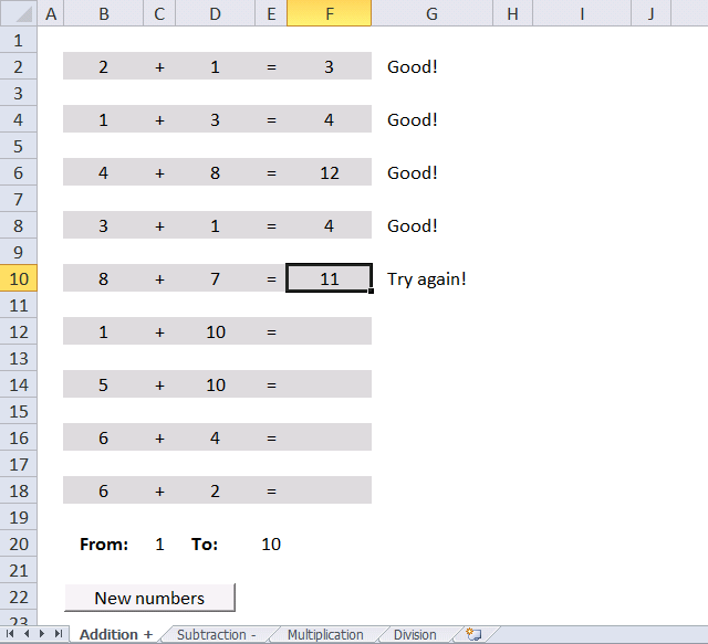
This section demonstrates a workbook that allows children to practice basic mathematics or more specifically arithmetic calculations. The image above shows a worksheet named "Addition", it allows the user to practice adding numbers.
There are four worksheets in the workbook and each worksheet shows numbers in columns B and D. The user then types the result in column F and Excel responds in column G if the answer was right or wrong.
Row 20 lets you control the numerical range that is used, for example, a range between 5 and 10 generates random whole numbers between 5 and 10 in column s B and D. This allows you to control the level of calculation, older children can use more difficult numbers to create a better challenge.
Row 22 contains a button that is linked to a macro named "Newnumbers()", press with left mouse button on the button to create new numbers in columns B and D.
The workbook contains four Excel worksheets named "Addition", "Subtraction", "Multiplication" and "Division". Press with mouse on one of the tabs below the cell grid to change the worksheet, shown in the image above.
Formula in cell B2:
This formula uses a User Defined Function that I created. It has two arguments, the lower bound and the upper bound specified in cell C20 and E20.
The VBA code for User Defined Function RandomBetween is shown below.
'Name UDF and dimension argument variables and declare data types
Function RandomBetween(Low As Long, High As Long)

'Initialize random-number generator
Randomize

'Create a whole random number based on arguments High and Low and return it to the cell in the worksheet
RandomBetween = Int(Rnd * (High - Low + 1)) + Low
End Function
Formula in cell G2:
The formula in cell G2 has two nested IF functions. The first IF function checks if cell F2 is empty and returns nothing if this is true. Another IF function is rund if this is false, it adds the numbers in cell B2 and D2 and checks if it is equal to the value in cell F2.
If they are equal then text string "Good!" is returned, if not equal text string "Try again" is returned.
The following macro clears cell range F2:F18 in all worksheets in the active workbook. This macro is used in all four worksheets and linked to a button in each worksheet.
'Name macro
Sub Newnumbers()

'Dimension variables and declare data types
Dim sht As Worksheet

'Iterate through each worksheet in active workbook using variable sht as worksheet
For Each sht In ActiveWorkbook.Worksheets

    'Clear cell range F2:F18 based on variable sht
    sht.Range("F2:F18") = ""

'Continue with next worksheet
Next sht

'Forces a full calculation of the data in all open workbooks.
Application.CalculateFull

End Sub
Subtraction
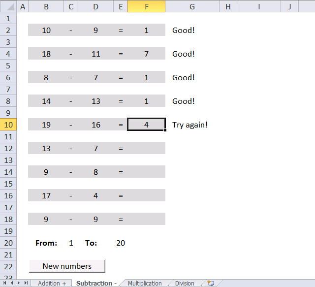
Worksheet "Subtraction" lets the user train their subtraction skills. The result is always 0 (zero) or higher. The same User Defined function is used in this worksheet as in worksheet "Addition", however, the second argument is different in column D.
Formula in cell B2:
Formula in cell D2:
If you want to allow negative results change the formula in column D to:
Formula in cell G2:
The formula in cell G2 has two nested IF functions. The first IF function checks if cell F2 is empty and returns nothing if this is true. Another IF function is rund if this is false, it subtracts the number in cell B2 with cell D2 and checks if it is equal to the value in cell F2.
If they are equal then text string "Good!" is returned, if not equal text string "Try again" is returned.
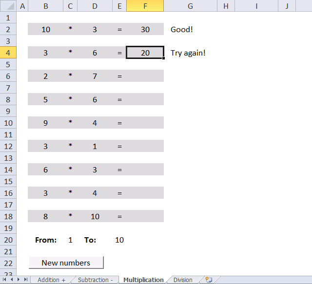
Multiplication
Formula in cell B2:
Formula in cell B2:
Formula in cell G2:
The formula in cell G2 has two nested IF functions. The first IF function checks if cell F2 is empty and returns nothing if this is true. Another IF function is rund if this is false, it multiplies the number in cell B2 with cell D2 and checks if it is equal to the value in cell F2.
If they are equal then text string "Good!" is returned, if not equal text string "Try again" is returned.
Division
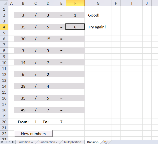
This worksheet contains math problems that lets you train divison. Dividend / Divisor = Quotient
This worksheet requires a different User Defined Function to avoid remainders. The number left over is called a remainder.
Formula in cell B2:
Formula in cell D2:
'Name user defined function and dimension parameters and their data types. Paramter Num is optional meaning it isn't required.
Function RandomBetweenDivison(Low As Long, High As Long, Optional Num As Variant)

'Dimension variables and declare data types
Dim i As Long, str() As Long

'The ReDim statement resizes a dynamic array that has already been declared
ReDim str(0)

'Initialize random-number generator
Randomize

'Check Optional variable Num is missing
If IsMissing(Num) Then

    'Create random whole numbers based on parameters High and Low
    RandomBetweenDivison = (Int(Rnd * (High - Low + 1)) + Low) * (Int(Rnd * (High - Low + 1)) + Low)
Else
    'Iterate from number stored in parameter Num to 1 based on -1 increments
    For i = Num To 1 Step -1

        'Check if paramater Num divided by variable i is a whole number
        If Num / i = Int(Num / i) Then

            'Save number in variable i to array variable str
            str(UBound(str)) = i

            'Add a new container to array variable str
            ReDim Preserve str(UBound(str) + 1)
        End If
    Next i

    'Delete last container in array variable str
    ReDim Preserve str(UBound(str) - 1)

    'Save random whole number based on the number of containers in array variable str to variable i
    i = Int(Rnd * (UBound(str)))

    'Return value stored in array variable str based on variable i
    RandomBetweenDivison = str(i)
End If
End Function
Where to put VBA code?

- Copy above VBA code.
- Press shortcut keys Alt + F11 to open the Visual Basic Editor.
- Press with mouse on "Insert" on the menu, see image above.
- Press with mouse on "Module".
- Paste VBA code to module window.
- Return to Excel.
Recommended links
Mathematics category
Solver category
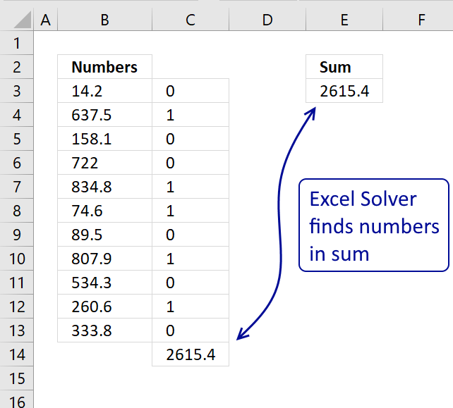
Table of Contents Identify numbers in sum using Excel solver Find numbers in sum - UDF Find positive and […]
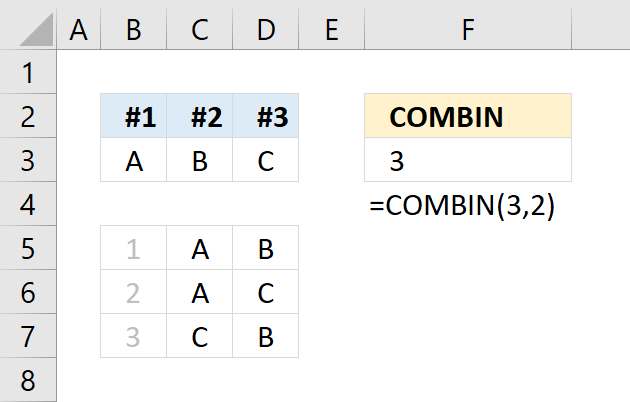
The COMBIN function returns the number of combinations for a specific number of elements out of a larger number of […]
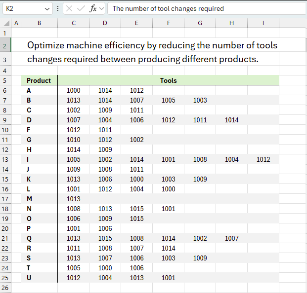
This article demonstrates solver in Excel. Table of Contents Introduction Optimize machine efficiency Using Excel Solver to schedule employees Cash […]
Excel categories
Leave a Reply
How to comment
How to add a formula to your comment
<code>Insert your formula here.</code>
Convert less than and larger than signs
Use html character entities instead of less than and larger than signs.
< becomes < and > becomes >
How to add VBA code to your comment
[vb 1="vbnet" language=","]
Put your VBA code here.
[/vb]
How to add a picture to your comment:
Upload picture to postimage.org or imgur
Paste image link to your comment.