How to use the SUM function
What is the SUM function?
The SUM function in Excel allows you to add numerical values and returning a total, the function returns the calculated sum in the cell it is entered in.
Does the SUM function ignore text and boolean values?
Yes, the SUM function is cleverly designed to ignore text and boolean values, adding only numbers.
Does the SUM function ignore error values?
No, the SUM function doesn't ignore error values. However, the AGGREGATE function allows you to calculate a total ignoring error values.
Table of Contents
- Syntax
- Arguments
- How to add numbers in a column and return a total (SUM function)?
- How to add numbers in an array (SUM function)?
- Specific cells
- Multiple cell ranges
- A column with text
- Adding boolean values
- Running total
- Based on a condition/label/item/category?
- Multiple conditions
- Only visible cells
- Filtered column
- Tthe entire column
- A row
- Add values across worksheets
- Create a total by color
- Absolute values
- How to use the SUM function in a macro - VBA example
- Shortcut key
- Add values greater than smaller than
- Add values below/above 0 (zero)?
- How to limit
- How to ignore errors
- Add values by date
- Add values by week
- Add values by month
- Add values by year
- Add values between two dates
- Reverse running total
- Add values based on check boxes
- Get Excel *.xlsm file
- Add selected values
- Add values in a column using a formula
- Add values in a given column using a formula
- Add values a given row using a formula
- Add values using an Excel defined Table
- Add cells containing numbers and text based on a condition
- Add unique numbers and return a total
- Function not working
1. Syntax
SUM(number1, [number2], ...)
2. Arguments
| number1 | Required. A constant, cell reference or an array that contains numerical values you want to add. |
| [number2] | Optional. Up to 254 additional arguments. |
The SUM function lets you add values in cell ranges, arrays, constants. You can have up to 255 different arguments.
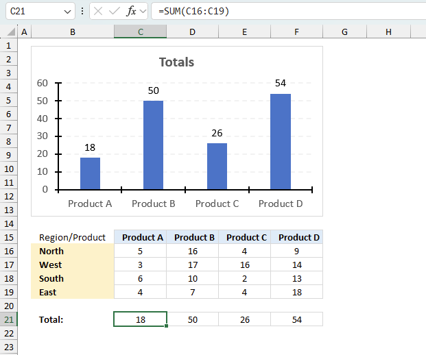
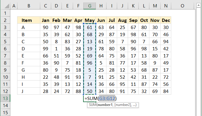
3. How to add numbers in a column
The SUM function lets you add values in a cell range, like this = SUM(B3:B7), instead of adding values in a formula using the plus sign, like this =B3+B4+B5+B6+B7.
The SUM function lets you type one or multiple cell ranges, in this example only cell range B3:B7 is entered as an argument. See the above picture.
Check out the shortcut key to automatically sum a column.
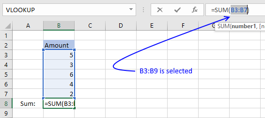
4. How to add numbers in an array
An array is multiple values enclosed with a beginning and ending curly bracket, you can easily convert a cell range to an array. See instructions below.
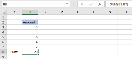
Select a cell and type =SUM(B3:B9)
Press with left mouse button on in the formula bar and select B3:B9.
Press F9 and the cell range is converted to an array, like this: =SUM({5,3,6,4,2})
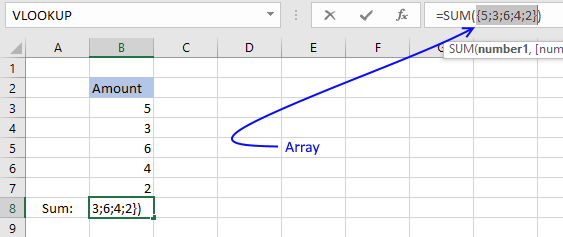
Press Enter.
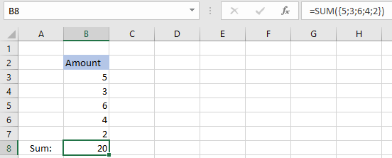
The SUM function adds the values in the array 5+3+6+4+2 = 20. When you convert a cell range to values you hard-code or create constants in your formula, meaning they never change unless you change the values in the formula.
Cell references on the other hand change if you change the values on a worksheet.
I recommend reading this post: Learn the basics of Excel arrays , if you want to learn more about array formulas.
5. How to add specific cells?

The SUM function allows you to add values from the cells you select. The trick is to press and hold the CTRL key while selecting specific cells to sum. Here are the steps in greater detail:
- Doublepress with left mouse button on a cell, the prompt shows up.
- Type =SUM(
- Press and hold CTRL-key.
- Press with left mouse button on with the left mouse button on cells you want to sum.
- Release CTRL-key.
- Add an ending parenthesis )
- Press Enter.

You can also sum cells based on a condition applied to an adjacent column.
6. How to add numbers in multiple cell ranges
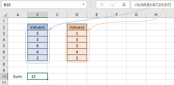
If you want to add values in multiple cell ranges you simply use a comma between arguments. Check your regional settings if a comma doesn't work for you. You are allowed to have up to 255 arguments in one SUM function.
- Doublepress with left mouse button on a cell, the prompt shows up.
- Type =SUM(
- Press and hold CTRL-key.
- Press and hold with the left mouse button.
- Drag with mouse to select the cell range.
- Release left mouse button.
- Go back to step 4 until all cell ranges have been selected.
- Release CTRL-key.
- Add an ending parenthesis )
- Press Enter.
7. How to add values in a column with text
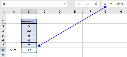
The formula in cell B8 adds the values in cell range B3:B7. 5 + AA + 6 + 4 +2 = 17. The SUM function ignores text strings, in this case AA.
The SUM function ignores text values and boolean values but not error values.
Note, the SUM function ignores numbers stored as text. The image below shows the SUM function in cell B8. Only number 4 is included in the total of cells in cell range B3:B7.

Excel shows numbers stored as text differently, see image above. Text values are aligned left in the cell and numbers are aligned right. Cells containing numbers stored as text show a green arrow in the upper left corner of the cell.
8. How to add boolean values
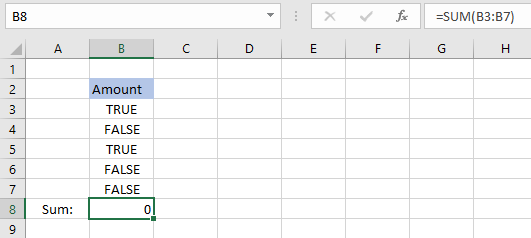
Cell range B3:B7 contains boolean values, TRUE or FALSE, however, the SUM function can't add boolean values unless they are converted to their numerical equivalents.
There are multiple solutions to this problem, here are a few:
Formula in cell B8:
Formula in cell B8:
Formula in cell B8:
They all convert boolean values to numerical values.
They need to be entered as array formula, because they do calculations to a cell range containing multiple cells.
Instructions on how to enter an array formula.
- Double press with left mouse button on cell B8
- Type =SUM(B3:B7*1)
- Press and hold CTRL + SHIFT simultaneously.
- Press Enter once.
- Release all keys.
The formula in the formula bar changes to {=SUM(B3:B7*1)}
These curly brackets tell you that you have created an array formula, don't enter these characters yourself.
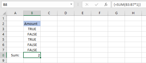
The formula returns 2 because TRUE equals 1 and FALSE equals 0. 1+0+1+0+0 = 2.
Note, you can use the SUMPRODUCT function if you don't want to use array formulas.
Regular formula in cell B8:
9. How to create a running total
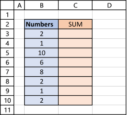
The image above shows you numbers in column B.
Enter this formula in cell C3:
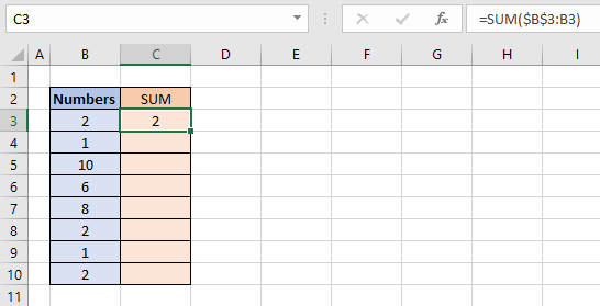
Make sure you get the dollar signs right, they are important. The cell reference changes as you copy the formula and paste it to cells below.
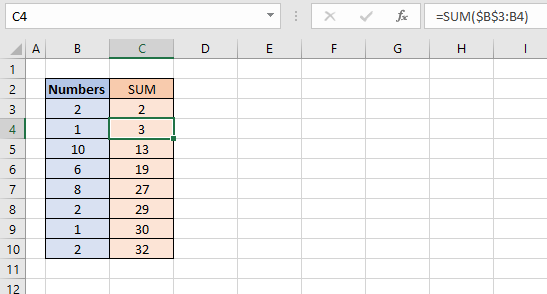
Select cell C4 and see how the formula changed in the formula bar. The part of the cell reference without dollar signs changed from B3 to B4.
That part is a relative cell reference and the part with dollar signs is an absolute cell reference.
Read more here: Absolute and relative cell references
This makes the SUM function use a cell reference that grows, in other words, it includes more and more cells creating a running total.
Formula in cell C4 adds numbers from both cell B3 and B4. The formula grows even further in cell C5 and it keeps growing in cells below.
Note, you can double press with left mouse button on the dot in the lower right corner of the cell to automatically copy the cell and paste it to cells below as far as there are populated cells in the adjacent column.

You can also easily create a reverse running total using two SUM functions, it adds values from the bottom going up to the top.
10. How to add values based on a condition
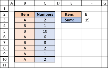
The picture above shows you two columns, column B contains text values and column C contains numbers. The formula demonstrated here allows you to sum by another column.
The formula in cell F3 lets you add numbers in column C if their adjacent value is equal to the value in cell F2:
This formula is entered as an array formula unless you are using Excel 365. I recommend the SUMIF function built exactly for this without entering the formula as an array formula.
Explaining formula in cell F3
Step 1 - Logical expression
The equal sign in B3:B10=F2 lets you compare the values in cell range B3:B10 with the value in cell F2. The equal sign is a logical operator, often used in IF functions.
{"A";"B";"B";"A";"B";"A";"A";"A"}="B"
This logical test returns an array of boolean values:
{FALSE; TRUE; TRUE; FALSE; TRUE; FALSE; FALSE; FALSE}
Step 2 - Multiply array with cell range
The parentheses (B3:B10=F2) make sure this part of the formula is calculated first before multiplying with the numbers in cell range C3:C10.
(B3:B10=F2)*C3:C10
FALSE is equal to 0 (zero) and TRUE is equal to 1.
returns {0; 1; 10; 0; 8; 0; 0; 0}
Step 3 - Sum numbers
The SUM function then adds the number in the array:
SUM({0; 1; 10; 0; 8; 0; 0; 0})
and returns 19 in cell F3. 1+10+8 = 19
Excel defined Table - SUM with criteria
11. Add values based on multiple conditions
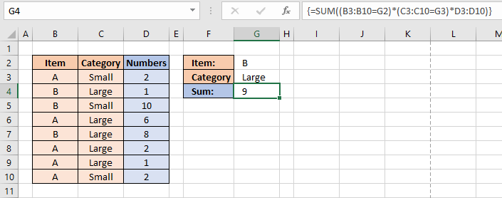
Adding a second condition to the formula is easy. Simply add your condition to the formula enclosed with parentheses.
This formula is entered as an array formula unless you are using Excel 365. I recommend the SUMIFS function built exactly for this without the need for an array formula.
Explaining formula in cell G4
Step 1 - First condition
The equal sign allows you to compare cells to each other.
B3:B10=G2
returns {FALSE; TRUE; ... ; FALSE}
Step 2 - Second condition
C3:C10=G3
returns {FALSE; TRUE; ... ; FALSE}
Step 3 - Multiply arrays
(B3:B10=G2)*(C3:C10=G3)*D3:D10
returns {0;1;0;0;8;0;0;0}
Step 4 - Sum values in the array
SUM((B3:B10=G2)*(C3:C10=G3)*D3:D10)
becomes SUM({0;1;0;0;8;0;0;0}) and returns 9.
The SUMPRODUCT function allows you to perform the same calculation without the need for entering the formula as an array formula.
12. How to add values based on visible cells
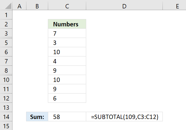
The SUBTOTAL function lets you sum values in a cell range that have some rows hidden or filtered, the picture above shows a cell range that has row 4 and 9 hidden. The usual SUM function won't work in this case, you need the SUBTOTAL function:
The first argument allows you to pick a function number that determines how the SUBTOTAL function behaves. In this case, 109 sums all visible cells in a cell range.
To hide a value simply press with right mouse button on on a row number and then press with left mouse button on "Hide" to hide the entire row. Select the rows around a hidden row and then press with right mouse button on on them to open a menu, there press with left mouse button on "Unhide" to show the value again.
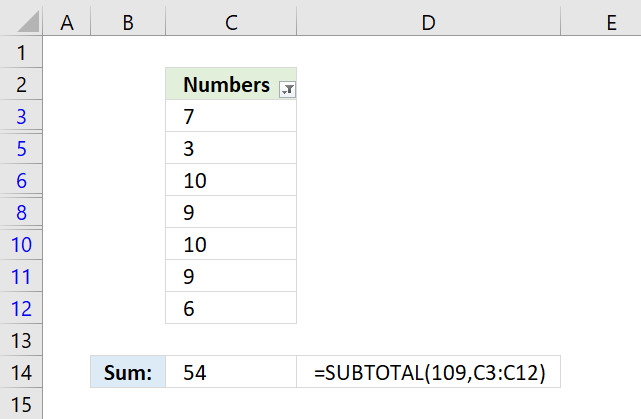
The picture above shows filtered values in column C. Excel tells you that the cell range is filtered by the color of the row numbers and the icon next to "Numbers" in cell C2.
To apply a filter to a column simply select the cell range, go to tab "Data" on the ribbon, press with left mouse button on "Filter" button. A black down-pointing arrow appears next to header name "Numbers", press with left mouse button on it to apply a filter.
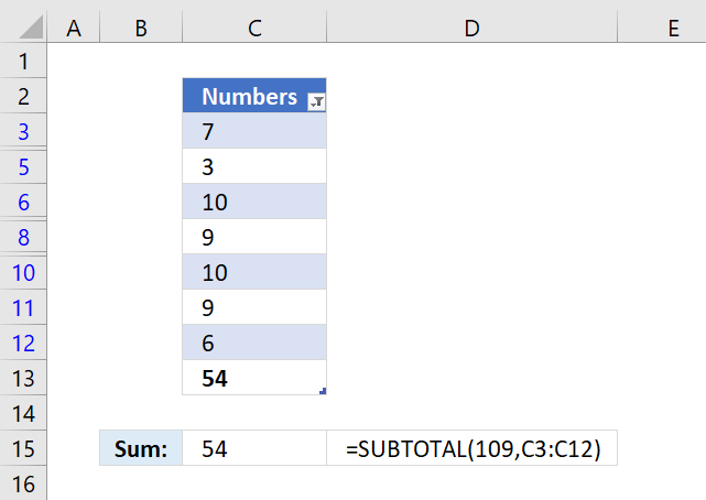
The Excel defined table above has a built-in feature that allows you to sum filtered values automatically, all you need to do is select a cell in the table, go to tab "Design" on the ribbon, then press with left mouse button on check-box "Total Row" to show the totals.
Cell C13 in the picture above displays the total for filtered cells. The SUBTOTAL function works just as well if you prefer using an Excel function with an Excel defined table, demonstrated in cell C15.
How to hide / unhide values?

Note, follow these instructions on how to hide and unhide specific rows:
- Press with right mouse button on on row number.
- A popup-menu appears, see image above.
- Press with mouse on Hide or Unhide.
Tip! Press and hold CTRL key while selecting rows to hide/unhide multiple values at the same time.
13. How to add values based on a filtered column?

The image above shows numbers in cell range C3:C7, however, a filter is applied and rows 4 and 6 are hidden. The SUM function in cell C9 can't ignore filtered values, you need the SUBTOTAL function to sum filtered numbers.
Formula in cell C10:
14. How to add values based on the entire column

The image above shows a formula that adds all values in a column and returns a total.
Formula in cell E2:
The cell reference is B:B meaning that all numerical values in column B are included in the total.
15. How to add values based on a row

The image above shows a formula that adds all values in a row and returns a total.
Formula in cell C4:
The cell reference is 2:2 meaning that all numerical values in row 2 are included in the total.
16. How to add values across worksheets

The image above shows a formula that adds values located in cell C3 across three different worksheets. For this to work values you want to add must be located in the same cell across all worksheets.
Formula in cell C3:
Here are the steps I did to create the formula above:
- Doublepress with left mouse button on cell C3, the prompt is shown.
- Type =SUM(
- Go to the first worksheet.
- Press with mouse on the cell containing the value you want to add.
- Press and hold SHIFT key.
- Select the last worksheet you want to include in the total.
- Release the SHIFT key.
- Type an ending parenthesis )
- Press Enter.
The image below shows the tabs I selected to create the formula above.

17. How to add values by color

The short answer is that there is really no way to sum by background color if you want to use formulas, however, a VBA macro can do it.
The long answer is that there is the GET.CELL function that has some serious flaws, one is that it is outdated and may be removed from Excel by Microsoft whenever they feel like it. I'd rather recommend coloring cells using Conditional Formatting and then using the same condition to sum the cells.
This is what the image above shows, I chose to highlight rows blue if the corresponding cell in column B is equal to item "B". Here is how I did it:
- Select the cells you want to highlight, in the example above cell range B3:C10.
- Go to tab "Home" on the ribbon.
- Press with left mouse button on the Conditional Formatting button.
- Press with left mouse button on "New Rule...". A dialog box appears.

- Press with mouse on "Use a formula to determine which cells to format"
- Press with mouse on field below "Format values where this formula is true:".
- Type =$B3=$F$2
- Press with left mouse button on "Format..." button. A new dialog box appears.

- Press with left mouse button on tab "Fill" on top menu.
- Pick a color.
- Press with left mouse button on OK. The dialog box is closed.
- Press with left mouse button on OK again.
The formula in cell F3 is explained here: How to sum numbers based on a condition/label/item/category?
18. How to sum absolute numbers

The image above shows a formula in cell C8 that converts negative values to positive values and then adds the values.
Formula in cell C8:
Explaining formula in cell C8
Step 1 - Remove sign
The ABS function converts negative numbers to positive numbers, in other words, the ABS function removes the sign.
ABS(number)
ABS(C3:C7)
returns {5; 3; 6; 4; 2}
Step 2 - Add values
SUM(ABS(C3:C7))
becomes
SUM({5; 3; 6; 4; 2})
and returns 20. 5+3+6+4+2 = 20
19. How to use the SUM function in a macro (VBA)?
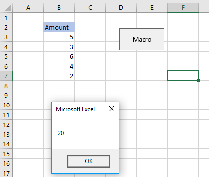
The image above demonstrates a macro that shows a message box with a number representing the total of cell range B3:B7.
'Macro name
Sub HLP()

'Show sum of B3:B7 in a messagebox
MsgBox Application.WorksheetFunction.Sum(Range("B3:B7"))

'Exit macro
End Sub
Microsoft docs: | Application.WorksheetFunction | Sum | Range | Msgbox
20. What is the shortcut key?

The animated image above shows how to add totals for a cell range, both vertically and horizontally, using a shortcut key.
The SUM formulas in cell range G3:G7 adds values from the cell to the left of the formula and on the same row.

The SUM formulas in cell range C7:F7 return a total based on the numbers above the formulas in the same column.

Here is how to create the SUM function using a shortcut key:
- Select the cell range containing numbers.
- Press and hold Alt key.
- Press the equal sign =
- Release the Alt key.
If the steps above don't work for you try Alt + Shift + 0 (zero) keys. It really depends on your keyboard layout which keys you need to press.

The ímage above shows that you can use the shortcut key below numbers in a column.
21. How to add values based on below/above a threshold

The image above demonstrates two array formulas in cell E3 and E5 that return a total with values larger or smaller than a given threshold.
Array formula in cell E3:
Array formula in cell E6:
I recommend the SUMIF function built exactly for this without entering the formula as an array formula.
Explaining formula in cell E3
Step 1 - Filter values above a threshold
The IF function returns one value if the logical test is TRUE and another value if the logical test is FALSE.
IF(logical_test, [value_if_true], [value_if_false])
IF(B3:B7>E2, B3:B7, )
becomes
IF({3;9;2;4;6}>5,{3;9;2;4;6},)
becomes
IF({FALSE; TRUE; FALSE; FALSE; TRUE},{3; 9; 2; 4; 6},)
and returns
{0;9;0;0;6}
Step 2 - Sum values
SUM(IF(B3:B7>E2, B3:B7, ))
becomes
SUM({0;9;0;0;6})
and returns 15 in cell E3.
Back to top
22. How to add values based on below/above 0 (zero)

The image above demonstrates two formulas in cells E2 and E3 that return a total with values above and below zero respectively.
Array formula in cell E2:
Array formula in cell E3:
I recommend the SUMIF function built exactly for this without entering the formula as an array formula.
Explaining formula in cell E2
Step 1 - Filter values above a 0 (zero)
The IF function returns one value if the logical test is TRUE and another value if the logical test is FALSE.
IF(logical_test, [value_if_true], [value_if_false])
IF(B3:B7>0, B3:B7, )
becomes
IF({1;-2;3;4;-3}>0,{1;-2;3;4;-3},)
becomes
IF({TRUE;FALSE;TRUE;TRUE;FALSE},{1;-2;3;4;-3},)
and returns
{1;0;3;4;0}
Step 2 - Sum numbers
SUM(IF(B3:B7>0, B3:B7, ))
becomes
SUM({1;0;3;4;0})
and returns 8 in cell E2. 1 + 3 + 4 = 8.
Back to top
23. How to create a limit

The image above demonstrates a formula in cell E3 that sums values in cell range B3:B7 and returns a total that is limited to the number specified in cell E2. In other words, the total can't be larger than the value in cell E2 but it can be smaller.
The image above also shows a formula in cell E6 that adds values in cell range B3:B7 and returns a total that is limited to the number specified in cell E5. The total can't be smaller than the value in cell E5 but it can be larger.
Formula in cell E3:
Formula in cell E6:
Explaining formula in cell E3
Step 1 - Sum numbers
SUM(B3:B7)
becomes
SUM({5;6;6;7;2})
and returns 26. 5+6+6+7+2=26
Step 2 - Return the smallest number
The MIN function returns the smallest number in a cell range or array.
MIN(E2, SUM(B3:B7))
becomes
MIN(20, 26)
and returns 20. 20 is smaller than 26.
24. How to ignore errors

The image above shows a formula in cell C9 that sums numbers in cell range C3:C7 and ignores errors.
Array Formula in cell C9:
Explaining formula in cell C9
Step 1 - Replace errors with 0 (zero)
The IFERROR function lets you handle most formula errors with ease.
IFERROR(value, value_if_error)
IFERROR(C3:C7, 0)
becomes
IFERROR({5;#DIV/0!;6;#NAME?;2})
and returns
{5;0;6;0;2}
Step 2 - Sum values in array
SUM(IFERROR(C3:C7, 0))
becomes
SUM({5;0;6;0;2})
and returns 13 in cell C9. 5+6+2=13
25. Calculate a total based on a date

The image above shows a formula in cell C11 that sums numbers in cell range C3:C7 if dates in B3:B7 are equal to C10.
Array formula in cell C11:
I recommend the SUMIF function built exactly for this without entering the formula as an array formula.
Explaining formula in cell C9
Step 1 - Logical expression
B3:B7=C10
becomes
{43831;43832;43833;43832;43835}=43832
and returns
{FALSE; TRUE; FALSE; TRUE; FALSE}
Step 2 - Evaluate IF function
The IF function returns one value if the logical test is TRUE and another value if the logical test is FALSE.
IF(B3:B7=C10, C3:C7, "")
becomes
IF({FALSE; TRUE; FALSE; TRUE; FALSE}, C3:C7, "")
becomes
IF({FALSE; TRUE; FALSE; TRUE; FALSE}, {1; 3; 5; 2; 4}, "")
and returns {""; 3; ""; 2; ""}.
Step 3 - Sum values in the array
SUM(IF(B3:B7=C10, C3:C7, ""))
becomes
SUM({""; 3; ""; 2; ""})
and returns 5. 3+2 = 5.
26. Calculate a total based on week number

The image above shows a formula in cell C11 that sums numbers in cell range C3:C7 if the corresponding weeks based on the dates in B3:B7 are equal to C10.
Array formula in cell C11:
I recommend the SUMIF function built exactly for this without entering the formula as an array formula.
Explaining formula in cell C9
Step 1 - Calculate week numbers
The ISOWEEKNUM function calculates the number of the ISO week number of the year for a specific date.
ISOWEEKNUM(B3:B7)
becomes
ISOWEEKNUM({43839; 43838; 43835; 43833; 43837})
and returns {2; 2; 1; 1; 2}
Step 2 - Logical expression
ISOWEEKNUM(B3:B7)=C10
becomes
{2; 2; 1; 1; 2}=1
and returns {FALSE; FALSE; TRUE; TRUE; FALSE}.
Step 3 - Evaluate IF function
The IF function returns one value if the logical test is TRUE and another value if the logical test is FALSE.
IF(ISOWEEKNUM(B3:B7)=C10, C3:C7, "")
returns {""; ""; 5; 2; ""}
Step 4 - Sum values in the array
SUM(IF(ISOWEEKNUM(B3:B7)=C10, C3:C7, ""))
becomes
SUM({""; ""; 5; 2; ""})
and returns 7. 5+2 = 7.
27. Calculate a total by month

The image above shows a formula in cell C11 that sums numbers in cell range C3:C7 if the corresponding weeks based on the dates in B3:B7 are equal to C10.
Array formula in cell C11:
I recommend the SUMIF function built exactly for this without entering the formula as an array formula.
Explaining formula in cell C9
Step 1 - Calculate number representing the position of the month in a year
The MONTH function extracts the month as a number from an Excel date.
1 - January, 2 - February, 3 - March, 4 - April, 5 - May, 6 - June, 7 - July, 8 - August, 9 - September, 10 - October, 11 - November, 12 - December
MONTH(B3:B7)
becomes
MONTH({43839; 43869; 43895; 43864; 43837})
returns
{1; 2; 3; 2; 1}
Step 2 - Logical expression
MONTH(B3:B7)=C10
becomes
{1; 2; 3; 2; 1}=1
and returns {TRUE; FALSE; FALSE; FALSE; TRUE}
Step 3 - Evaluate IF function
The IF function returns one value if the logical test is TRUE and another value if the logical test is FALSE.
IF(MONTH(B3:B7)=C10, C3:C7, "")
becomes
IF({TRUE; FALSE; FALSE; FALSE; TRUE}, {1; 3; 5; 2; 4}, "")
and returns {1; ""; ""; ""; 4}
Step 4 - Sum values in the array
SUM(IF(MONTH(B3:B7)=C10, C3:C7, ""))
becomes
SUM({1; ""; ""; ""; 4})
and returns 5. 1 + 4 = 5.
28. Calculate a total by year

The image above shows a formula in cell C11 that sums numbers in cell range C3:C7 if the corresponding weeks based on the dates in B3:B7 are equal to C10.
Array formula in cell C11:
I recommend the SUMIF function built exactly for this without entering the formula as an array formula.
Explaining formula in cell C9
Step 1 - Calculate year based on an Excel date
The YEAR function returns the year from an Excel date.
YEAR(B3:B7)
becomes
YEAR({44205; 43869; 44260; 43864; 44568})
and returns {2021; 2020; 2021; 2020; 2022}
Step 2 - Logical expression
YEAR(B3:B7)=C10
becomes
{2021; 2020; 2021; 2020; 2022}=2020
and returns {FALSE; TRUE; FALSE; TRUE; FALSE}
Step 3 - Evaluate IF function
The IF function returns one value if the logical test is TRUE and another value if the logical test is FALSE.
IF(YEAR(B3:B7)=C10, C3:C7, "")
becomes
IF({FALSE; TRUE; FALSE; TRUE; FALSE}, {1; 3; 5; 2; 4}, "")
and returns {""; 3; ""; 2; ""}
Step 4 - Sum values in array
SUM(IF(YEAR(B3:B7)=C10, C3:C7, ""))
becomes
SUM({""; 3; ""; 2; ""})
and returns 5. 3 + 2 = 5.
29. Calculate a total based on values between two dates

The image above shows a formula in cell C12 that sums numbers in cell range C3:C7 if dates in B3:B7 are less than or equal to C11 and greater than or equal to C10.
Array formula in cell C12:
I recommend the SUMIFS function built exactly for this without entering the formula as an array formula.
Explaining formula in cell C9
Step 1 - First logical expression
C10<=B3:B7
becomes
43832<={43831; 43832; 43833; 43834; 43835}
and returns
{FALSE; TRUE; TRUE; TRUE; TRUE}
Step 2 - Second logical expression
C11>=B3:B7
becomes
43834>={43831;43832;43833;43834;43835}
and returns
{TRUE; TRUE; TRUE; TRUE; FALSE}
Step 3 - Multiply arrays
(C10<=B3:B7)*(C11>=B3:B7)
becomes
{FALSE; TRUE; TRUE; TRUE; TRUE}*{TRUE; TRUE; TRUE; TRUE; FALSE}
and returns {0; 1; 1; 1; 0}
Step 4 - Evaluate IF function
The IF function returns one value if the logical test is TRUE and another value if the logical test is FALSE.
IF((C10<=B3:B7)*(C11>=B3:B7), C3:C7, "")
returns {""; 3; 5; 2; ""}
Step 5 - Sum values in the array
SUM(IF((C10<=B3:B7)*(C11>=B3:B7), C3:C7, ""))
becomes
SUM({""; 3; 5; 2; ""})
and returns 10. 3+5+2 = 10.
30. How to create a reverse running total

The image above shows a formula in cell C3 that calculates a running total from the bottom to the top and not the other way around.
Formula in cell C3:
Explaining the formula in cell C3
Step 1 - Calculate the total for the entire cell range
The SUM function allows you to add numerical values, the function returns the sum in the cell it is entered in. The SUM function is cleverly designed to ignore text and boolean values, adding only numbers.
Function syntax: SUM(number1, [number2], ...)
SUM($B$3:$B$7)
becomes
SUM({5;4;8;6;1})
and returns
24.
Step 2 - Calculate a running total using absolute and relative cell references
SUM($B$2:B2)
The dollar sign lets you change a relative cell reference to an absolute cell reference, this makes the cell reference grow automatically as the cell is copied to the cells below.
Cell C3: SUM($B$2:B2)
Cell C4: SUM($B$2:B3)
Cell C5: SUM($B$2:B4)
Cell C6: SUM($B$2:B5)
Cell C7: SUM($B$2:B6)
Step 3 - Subtract the total with the running total
The minus sign lets you subtract numbers in an Excel formula.
SUM($B$3:$B$7)-SUM($B$2:B2)
becomes
Cell C3: 24-0 equals 24
Cell C4: 24-5 equals 19
Cell C5: 24-9 equals 15
Cell C6: 24-17 equals 7
Cell C7: 24-23 equals 1
The file is a *.xlsm file (macro-enabled Excel file), it contains a small macro that demonstrates how to use the SUM function in a VBA macro.
31. Calculate a total based on check boxes
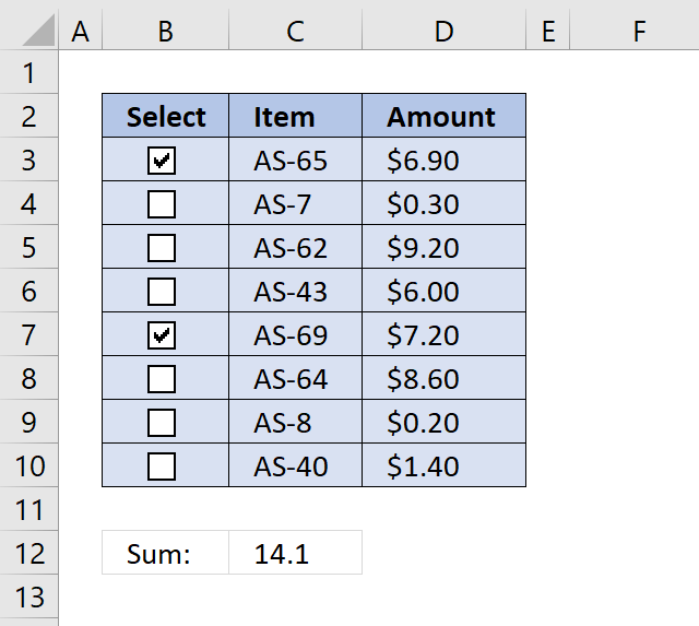
I will now demonstrate with the following table how to add check-boxes and sum enabled check-boxes using a formula.
31.1 Add check boxes to worksheet
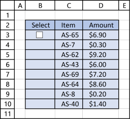
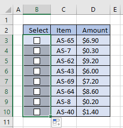
The following animated image shows you how to quickly insert and position a check box, then easily copy and paste it to cells below.
The picture above doesn't show you how to link check boxes and hide linked cell values, detailed instructions below:
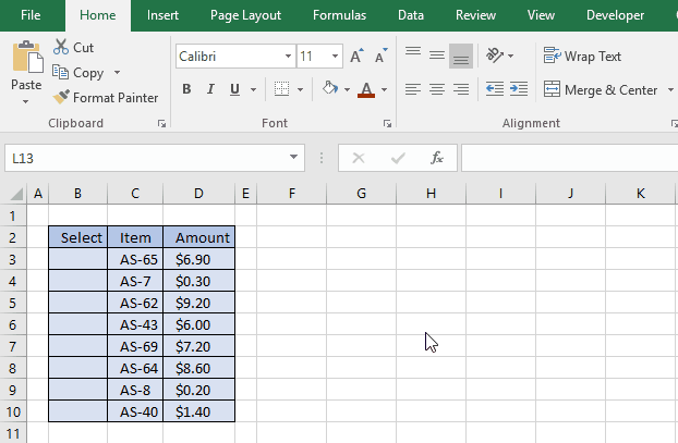
Select cell B3. Go to tab "Developer" and and press with left mouse button on "Insert" button and then "Check boxes (form control)".
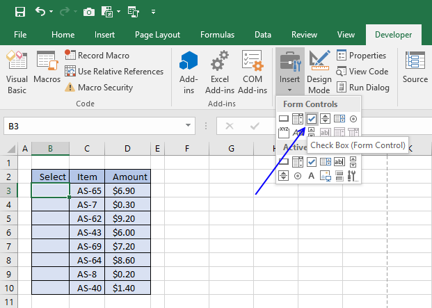
Draw a check box in cell B3. Remove check box text. Use arrow keys to position checkbox 1 px incrementally.
Press and hold with left mouse button black box in the bottom right corner of cell B3.
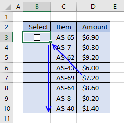
Drag down as far as needed, in this example to cell B10.
The following article shows you a template that allows you construct multi-level to-do lists:
Recommended articles
Today I will share a To-do list excel template with you. You can add text to the sheet and an […]
31.2 Link check boxes to cells
Press with right mouse button on on check box in cell B3, press with left mouse button on "Format Control..."
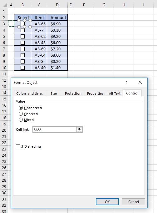
Press with mouse on Cell link: field and select cell A3, press with left mouse button on OK button.
Repeat this with check box in cell B4 and select cell link cell A4.
Now repeat this with remaining check-boxes in cell range B5:B10.
31.3 Hide values in cell range A3:A10
Select cell A3:A10. Press CTRL + 1.
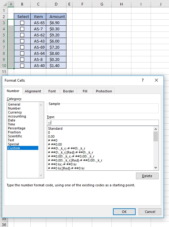
Press with left mouse button on "Custom" category, see picture above. Type ;;; in type field, see picture above. Press with left mouse button on OK button.
Recommended article:
Recommended articles
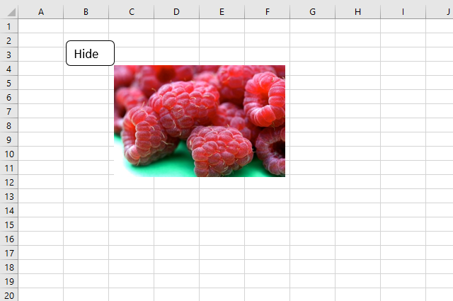
This article explains how to hide a specific image in Excel using a shape as a button. If the user […]
31.4 Build formula
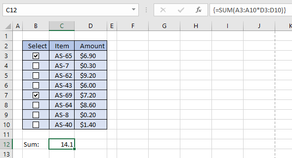
Double press with left mouse button on cell C12. Type:
Recommended article:
Recommended articles
What is the SUM function? The SUM function in Excel allows you to add numerical values and returning a total, […]
Create an array formula, see instructions below.
- Press CTRL + SHIFT simultaneously
- Press Enter once
- Release all keys
If you did this right the formula now has a beginning and ending curly bracket, like this: {=SUM(A3:A10*D3:D10)}
Don't enter these characters yourself, they appear automatically.
Check a few check boxes to verify that the formula is working.
If you don't like array formulas, use this formula:
Get excel *.xlsx file
Useful links
SUM function - Microsoft
5 ways to sum a column in Excel
I will in this article demonstrate different ways to sum values, the first method is so easy and fast it's ridiculous.
33. How to create a total based on selected values
The easiest way to sum a cell range is to simply select the cell range and read the values in the status bar. It shows the total, the count of non-empty cells and the average.
In fact, you can customize the status bar to show even more data:
Here is how to show these calculations automatically in the status bar.
- Press with right mouse button on on the status bar with your mouse.
- Press with left mouse button on "Numerical Count", "Minimum", and "Maximum", see image below.
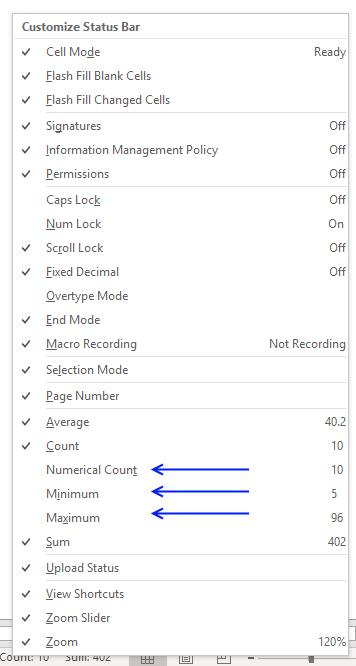
The image below demonstrates these calculations enabled.
34. Add values in a column using a formula
This is probably the most common task in Excel and luckily, there is an easy short cut to use.
- Select the cell range you want to sum.
- Press and hold Alt on your keyboard.
- Then press =
This will create a formula containing the SUM function and a cell reference to the selected cells, see image above.
You can also go to tab "Home" on the ribbon and press with left mouse button on "AutoSum" button and get the same result. To create totals below all columns select cell range C13:N13 and press and hold Alt and then press =
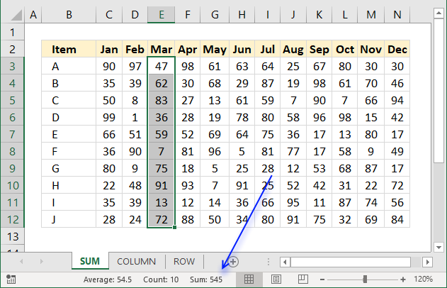
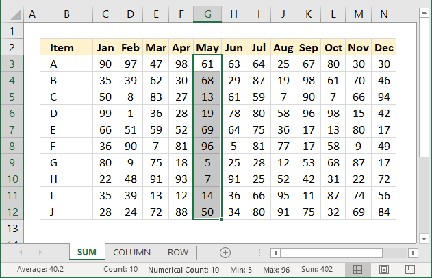
35. Add values in a given column using a formula
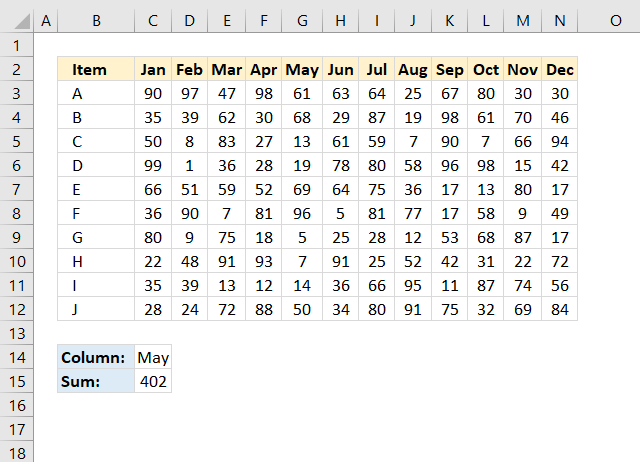
The picture above shows a formula in cell C15 that sums a column in cell range C3:N12 based on the specified column header in cell C14.
Formula in cell C15:
Explaining formula in cell C15
The MATCH function returns a number representing the position of the given value in cell C14, in C2:N2.
MATCH(C14, C2:N2, 0)
becomes
MATCH("May", {"Jan", ... , "Dec"}, 0)
and returns 5.
The INDEX function returns the entire column in cell C3:N12 if the row argument is 0 (zero).
INDEX(C3:N12, 0, MATCH(C14, C2:N2, 0))
becomes
INDEX(C3:N12, 0, 5)
and returns {61; 68; 13; 19; 69; 96; 5; 7; 14; 50}.
The SUM function adds the numbers given and returns a total.
SUM(INDEX(C3:N12, 0, MATCH(C14, C2:N2, 0)))
becomes
SUM({61; 68; 13; 19; 69; 96; 5; 7; 14; 50})
and returns 402.
36. Add values in a given row using a formula
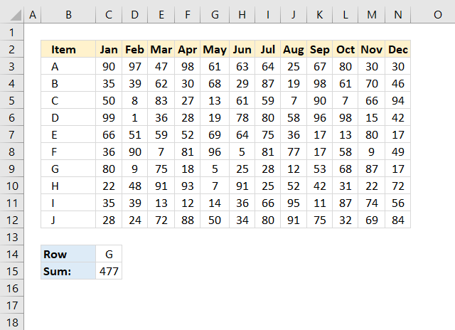
Formula in cell C15:
This formula is very similar to the prior one, no explanation is needed.
37. Add values in an Excel defined Table
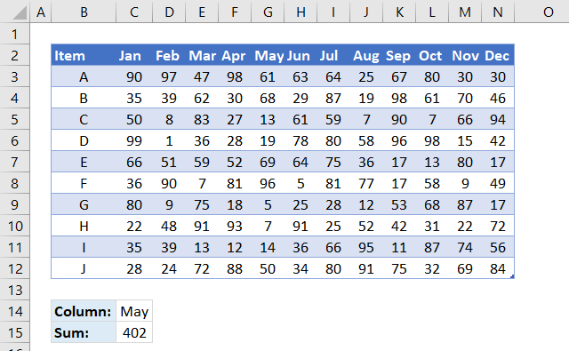
This image displays the dataset converted to an Excel defined Table. When you press with left mouse button on and drag to create cell references they are instantly changed to structured references, this means that you generally don't have to adjust the cell references when you add data to the Excel defined Table.
Formula in cell C15:
38. Add cells containing numbers and text based on a condition
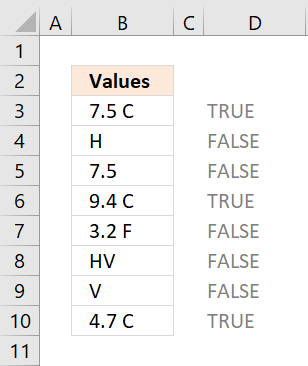
Question:
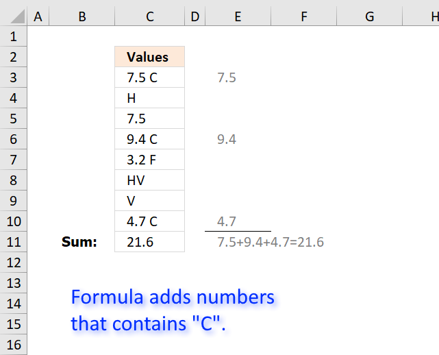
I want to sum cells that have a "C" and a decimal number.
The cells have other numbers and variables in them as well, but I only want to add ones
with "C"s.
Example of what cells contain:
7.5 C
H
7.5
9.4 C
3.2 F
HV
V
4.7 C
Answer:
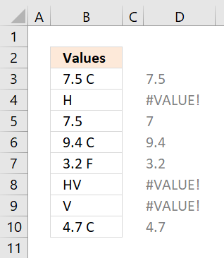
The array formula in the picture above searches for string "C" in cell range C3:C10 and extracts the corresponding number part.
Then it adds
Array formula in cell C11:
To enter an array formula, type the formula in cell B3 then press and hold CTRL + SHIFT simultaneously, now press Enter once. Release all keys.
 The formula bar now shows the formula with a beginning and ending curly bracket telling you that you entered the formula successfully.
Don't enter the curly brackets yourself, they appear automatically.
Explaining formula
Use "Evaluate Formula" on tab "Formula" on the ribbon to go through the steps in the formula.
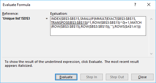
Step 1 - Find values containing text string
The SEARCH function allows you to search for a specific string in a cell range or array.
 SEARCH("C", C3:C10)
returns {5; #VALUE!; ... ; 5}.
The issue with this array is that the SEARCH function returns a #VALUE error if the string is not found.
Number 5 is where "C" is found in the string, in other words "C" is found in position 5 counting from the left.
For example, 7.5 C has five characters, "C" is the fifth character in the string.
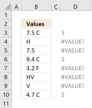
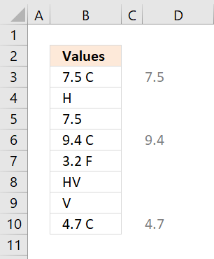
Step 2 - Identify numbers in array
The ISNUMBER function handles error values in a great way, instead of returning the error value it converts it to FALSE.
 ISNUMBER(SEARCH("C", C3:C10))
becomes
ISNUMBER({5; #VALUE!; ...; 5})
and returns {TRUE; FALSE; ....; TRUE}.
We now have an array without error values that is easier to work with.
TRUE indicates that the corresponding cell contains the string "C" and FALSE that "C" is missing.
Step 3 - Remove C from value and convert it to a numerical value.
Since C is the last character we can use the LEFT function to extract a given number of characters.
 The LEN function counts the number of characters in each cell. Subtracting with 1 returns how many characters we need to extract counting from left.
LEFT(C3:C10, LEN(C3:C10)-1)*1
becomes
LEFT(C3:C10, {4; 0; 2; 4; 4; 1; 0; 4})*1
becomes
{"7.5 ";"";"7.";"9.4 ";"3.2 ";"H";"";"4.7 "}*1
To convert text values to numerical values I multiply with 1.
{"7.5 "; ""; "7."; "9.4 "; "3.2 "; "H"; ""; "4.7 "}*1
becomes
{7.5; #VALUE!; 7; 9.4; 3.2; #VALUE!; #VALUE!; 4.7}
We can now use this array to replace the boolean array if value is TRUE.
Step 4 - Convert boolean values to corresponding numbers
The IF function allows you to use the boolean array and replace it with numbers (if TRUE) or nothing (if FALSE).
 IF(ISNUMBER(SEARCH("C", C3:C10)), LEFT(C3:C10, LEN(C3:C10)-1)*1, "")
returns {7.5; ""; ""; 9.4; ""; ""; ""; 4.7}.
The error values are ignored and "" (nothing) is returned in those locations.
Step 5 - SUM numerical values ignoring blank values
The SUM function is intelligent, it ignores blank and text values.
SUM(IF(ISNUMBER(SEARCH("C", C3:C10)), LEFT(C3:C10, LEN(C3:C10)-1)*1, ""))
becomes
SUM({7.5; ""; ""; 9.4; ""; ""; ""; 4.7})
and returns 21.6 in cell C11.
39. Add unique numbers and return a total
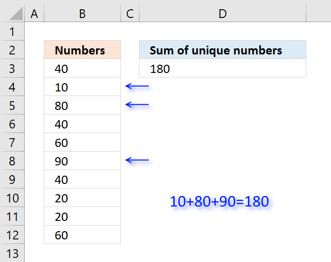
Table of Contents
- Sum unique numbers
- Get Excel *.xlsx file
- Sum unique distinct numbers
- Get Excel *.xlsx file
- Sum number based on corresponding unique value
39.1. Sum unique numbers
The formula in cell D3 adds all unique numbers in cell range B3:B12 and returns the total. Unique values are all values occurring only once in the list.
Formula in cell D3:
Excel 365 formula:
Explaining formula in cell D3
Step 1 - Count occurrence of each value in cell range
The COUNTIF function is an extremely useful function, this time I am counting how many times each value shows up in the cell range.
COUNTIF(B3:B12,B3:B12)
returns {3;1;1;3;2;1;3;2;2;2}
Step 2 - Check if value is unique
The equal sign checks if number is equal to 1.
COUNTIF(B3:B12,B3:B12)=1
returns {FALSE; ... ; FALSE}
Step 3 - Multiply with cell range
The boolean values in the array show which numbers to include in sum. FALSE is the same as 0 (zero) and TRUE is equivalebt to 1. The parentheses make sure that the comparison is calculated before multiplying.
(COUNTIF(B3:B12,B3:B12)=1)*B3:B12
returns {0;10;80;0;0;90;0;0;0;0}
Step 4 - Sum numbers
The SUMPRODUCT function now simply adds the numbers and returns the total.
SUMPRODUCT((COUNTIF(B3:B12,B3:B12)=1)*B3:B12)
becomes SUMPRODUCT({0;10;80;0;0;90;0;0;0;0}) and returns 180 in cell D3.
Why use the SUMPRODUCT function and not the SUM function? You don't need to enter this formula as an array formula if you use the SUMPRODUCT function.
Get Excel *.xlsx file
39.2. Sum unique distinct numbers
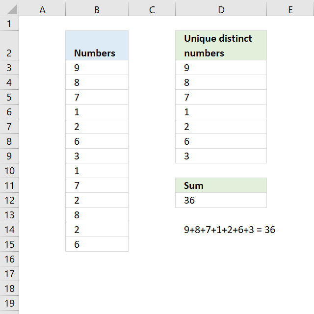
The image above shows numbers in column B, some of these numbers are duplicates. The formula in D12 adds unique distinct numbers meaning the first instance of each number is added to the total, however, the duplicates are ignored.
Excel 365 dynamic array formula:
Explaining formula in cell D12
If you want to examine the formula yourself then go to tab "Formula" on the ribbon and then press with left mouse button on "Evaluate Formula" button.
This will show the calculation steps, one at a time. Simply press with left mouse button on the Evaluate button to move to next calculation step.
Step 1 - Count each value in cell range
The COUNTIF function counts each value in the cell range and returns an array of numbers which shows the number of instances each value has.
COUNTIF(B3:B15,B3:B15)
returns {1;2;2;2;3;2;1;2;2;3;2;3;2}.
Step 2 - Divide 1 with array
If a number has a duplicate then there are two instances of that value. Divide 1 with 2 and we get 0.5, now multiply that value with the number and we get the number to add to the total.
1/COUNTIF(B3:B15,B3:B15)
returns {1;0.5;...;0.5}
Step 3 - Multiply with numbers
The parentheses make sure that the order of calculation is correct.
(1/COUNTIF(B3:B15,B3:B15))*B3:B15
returns {9;4;... ;3}
Step 4 - Add numbers
The SUMPRODUCT function is a better option than the SUM function, we don't need to enter the formula as an array formula now.
SUMPRODUCT((1/COUNTIF(B3:B15,B3:B15))*B3:B15)
becomes
SUMPRODUCT({9;4;3.5;0.5;0.666666666666667;3;3;0.5;3.5;0.666666666666667;4;0.666666666666667;3})
and returns 36 in cell D12.
Get Excel *.xlsx file
Sum unique distinct numbers.xlsx
39.3. Sum number based on the corresponding unique value
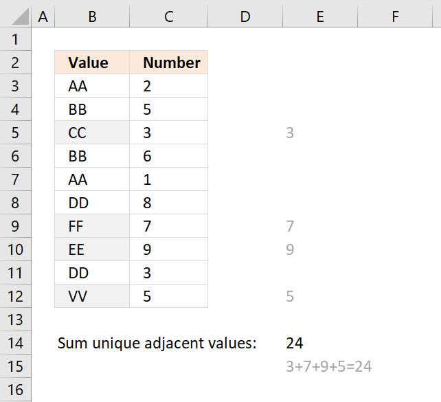
The formula in cell E14 adds a number from column C if the corresponding value in column B is unique and returns the total for all unique values. Unique values are values that exist only once in the list, in other words, there is only one instance of the value.
Formula in cell E14:
Explaining formula in cell E14
Step 1 - Count values in column B
The COUNTIF function counts values based on a condition, I am using multiple conditions, in this case.
COUNTIF($B$3:$B$12,$B$3:$B$12)
returns {2;2;... ;1}
Step 2 - Check if unique
The equal sign compares each value in the array to 1 and returns either TRUE or FALSE.
COUNTIF($B$3:$B$12,$B$3:$B$12)=1
returns {FALSE; FALSE; ... ; TRUE}
Step 3 - Multiply with numbers in column C
(COUNTIF($B$3:$B$12,$B$3:$B$12)=1)*$C$3:$C$12
returns {0;0;3;0;0;0;7;9;0;5}
Step 4 - SUM numbers
The SUMPRODUCT function then adds the numbers and returns the total to cell E14.
SUMPRODUCT((COUNTIF($B$3:$B$12,$B$3:$B$12)=1)*$C$3:$C$12)
becomes SUMPRODUCT({0;0;3;0;0;0;7;9;0;5}) and returns 24 in cell E14.
40. Function not working
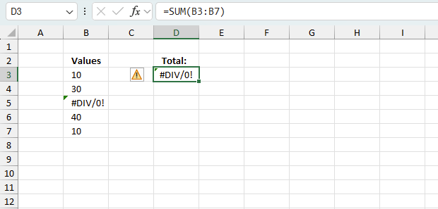
The SUM function returns
- #NAME? error if you misspell the function name.
- propagates errors, meaning that if the input contains an error (e.g., #VALUE!, #REF!, #DIV/0), the function will return the same error.
40.1 Troubleshooting the error value
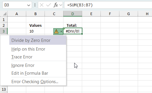
When you encounter an error value in a cell a warning symbol appears, displayed in the image above. Press with mouse on it to see a pop-up menu that lets you get more information about the error.
- The first line describes the error if you press with left mouse button on it.
- The second line opens a pane that explains the error in greater detail.
- The third line takes you to the "Evaluate Formula" tool, a dialog box appears allowing you to examine the formula in greater detail.
- This line lets you ignore the error value meaning the warning icon disappears, however, the error is still in the cell.
- The fifth line lets you edit the formula in the Formula bar.
- The sixth line opens the Excel settings so you can adjust the Error Checking Options.
Here are a few of the most common Excel errors you may encounter.
#NULL error - This error occurs most often if you by mistake use a space character in a formula where it shouldn't be. Excel interprets a space character as an intersection operator. If the ranges don't intersect an #NULL error is returned. The #NULL! error occurs when a formula attempts to calculate the intersection of two ranges that do not actually intersect. This can happen when the wrong range operator is used in the formula, or when the intersection operator (represented by a space character) is used between two ranges that do not overlap. To fix this error double check that the ranges referenced in the formula that use the intersection operator actually have cells in common.
#SPILL error - The #SPILL! error occurs only in version Excel 365 and is caused by a dynamic array being to large, meaning there are cells below and/or to the right that are not empty. This prevents the dynamic array formula expanding into new empty cells.
#DIV/0 error - This error happens if you try to divide a number by 0 (zero) or a value that equates to zero which is not possible mathematically.
#VALUE error - The #VALUE error occurs when a formula has a value that is of the wrong data type. Such as text where a number is expected or when dates are evaluated as text.
#REF error - The #REF error happens when a cell reference is invalid. This can happen if a cell is deleted that is referenced by a formula.
#NAME error - The #NAME error happens if you misspelled a function or a named range.
#NUM error - The #NUM error shows up when you try to use invalid numeric values in formulas, like square root of a negative number.
#N/A error - The #N/A error happens when a value is not available for a formula or found in a given cell range, for example in the VLOOKUP or MATCH functions.
#GETTING_DATA error - The #GETTING_DATA error shows while external sources are loading, this can indicate a delay in fetching the data or that the external source is unavailable right now.
40.2 The formula returns an unexpected value
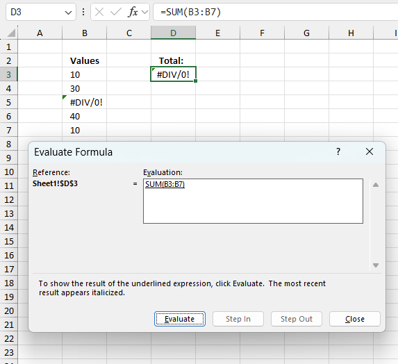
To understand why a formula returns an unexpected value we need to examine the calculations steps in detail. Luckily, Excel has a tool that is really handy in these situations. Here is how to troubleshoot a formula:
- Select the cell containing the formula you want to examine in detail.
- Go to tab “Formulas” on the ribbon.
- Press with left mouse button on "Evaluate Formula" button. A dialog box appears.
The formula appears in a white field inside the dialog box. Underlined expressions are calculations being processed in the next step. The italicized expression is the most recent result. The buttons at the bottom of the dialog box allows you to evaluate the formula in smaller calculations which you control. - Press with left mouse button on the "Evaluate" button located at the bottom of the dialog box to process the underlined expression.
- Repeat pressing the "Evaluate" button until you have seen all calculations step by step. This allows you to examine the formula in greater detail and hopefully find the culprit.
- Press "Close" button to dismiss the dialog box.
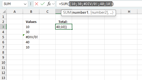
There is also another way to debug formulas using the function key F9. F9 is especially useful if you have a feeling that a specific part of the formula is the issue, this makes it faster than the "Evaluate Formula" tool since you don't need to go through all calculations to find the issue.
- Enter Edit mode: Double-press with left mouse button on the cell or press F2 to enter Edit mode for the formula.
- Select part of the formula: Highlight the specific part of the formula you want to evaluate. You can select and evaluate any part of the formula that could work as a standalone formula.
- Press F9: This will calculate and display the result of just that selected portion.
- Evaluate step-by-step: You can select and evaluate different parts of the formula to see intermediate results.
- Check for errors: This allows you to pinpoint which part of a complex formula may be causing an error.
The image above shows cell reference B3:B7 converted to hard-coded value using the F9 key. The SUM function requires non-error values which is not the case in this example. We have found what is wrong with the formula.
Tips!
- View actual values: Selecting a cell reference and pressing F9 will show the actual values in those cells.
- Exit safely: Press Esc to exit Edit mode without changing the formula. Don't press Enter, as that would replace the formula part with the calculated value.
- Full recalculation: Pressing F9 outside of Edit mode will recalculate all formulas in the workbook.
Remember to be careful not to accidentally overwrite parts of your formula when using F9. Always exit with Esc rather than Enter to preserve the original formula. However, if you make a mistake overwriting the formula it is not the end of the world. You can “undo” the action by pressing keyboard shortcut keys CTRL + z or pressing the “Undo” button
40.3 Other errors
Floating-point arithmetic may give inaccurate results in Excel - Article
Floating-point errors are usually very small, often beyond the 15th decimal place, and in most cases don't affect calculations significantly.
Get Excel *.xlsx file
Sum only if unique value in another column.xlsx
'SUM' function examples

Table of Contents Automate net asset value (NAV) calculation on your stock portfolio Calculate your stock portfolio performance with Net […]
This article explains how to calculate an overlapping time ranges across multiple days. This can be very useful in situations […]
Table of Contents How to use the BETADIST function How to use the BETAINV function How to use the BINOMDIST […]
Functions in 'Math and trigonometry' category
The SUM function function is one of 62 functions in the 'Math and trigonometry' category.
Excel function categories
Excel categories
3 Responses to “How to use the SUM function”
Leave a Reply
How to comment
How to add a formula to your comment
<code>Insert your formula here.</code>
Convert less than and larger than signs
Use html character entities instead of less than and larger than signs.
< becomes < and > becomes >
How to add VBA code to your comment
[vb 1="vbnet" language=","]
Put your VBA code here.
[/vb]
How to add a picture to your comment:
Upload picture to postimage.org or imgur
Paste image link to your comment.
Great Tutorial Oscar! I'm using the check box in an Excel sheet thanks to you. Just wondering, is there a way to multiply the values in column C, rows 1 through 5 by any value I chose? Say row 1, when checked, could be multiplied by a value of 2 and row 4 when checked multiplied by a value of 5. If I could add the ability to select "quantities of" for each row that'd be great.
Randal,
Yes, it is possible. If column D in the example above contains quantities the formula in cell C8 becomes:
=SUMPRODUCT(($B$1:$B$5=TRUE)*$C$1:$C$5*$D$1:$D$5)
Good stuff! A couple of questions: I am trying to sum the number of checked boxes in a row in excel. I have quite a few and want to avoid having individual format controls for each cell. Is there an easier way to do this? Is there a way to copy and paste format controls across multiple cells?
thanks