How to use the AVERAGEIF function
What is the AVERAGEIF function?
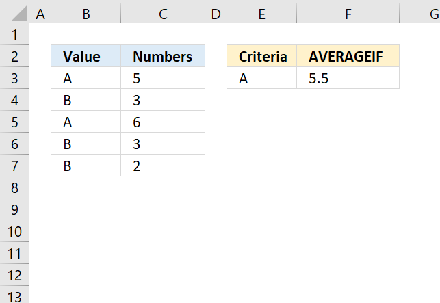
The AVERAGEIF function returns the average of cell values that are valid for a given condition. The AVERAGEIF function is available for Excel 2010 users and later versions.
Table of Contents
1. Syntax
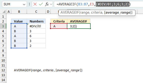
AVERAGEIF(range, criteria, [average_range])
2. Arguments
| range | Required. One or more cells to average, including numbers or names, arrays, or references that contain numbers. |
| criteria | Required. A cell reference, expression or text that determines which values to be evaluated. |
| average_range | Optional. Cells to average. If not entered, range is used. |
3. Which values are excluded?

- The AVERAGIF function excludes Boolean values TRUE or FALSE in the calculation, see the example in cell C5 in the image above.
Cell C5 contains the boolean value TRUE, the corresponding value in cell B5 matches the condition specified in cell E3. The boolean value TRUE is ignored nonetheless. - Empty blank cells in argument average_range is excluded from the calculation, see cell C3 in the picture above, despite the matching corresponding value in cell B3.
4. Function not working
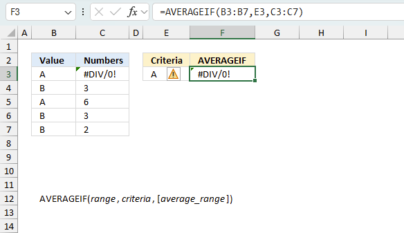
- The AVERAGEIF function returns #DIV0! if no values match the criteria.
- A #NAME error translates to a misspelled function in your formula.
- The AVERAGEIF function ignores text and boolean values, however, not error values.
- Trying to use an asterisk or question mark as a condition? It won't work as they are wildcard characters, however, there is a workaround. Use the ~ (tilde) character to escape wildcard characters.
- propagates errors meaning an error is returned if an error exists in the source data range.
4.1 Troubleshooting the error value
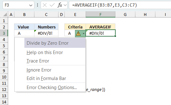
When you encounter an error value in a cell a warning symbol appears, displayed in the image above. Press with mouse on it to see a pop-up menu that lets you get more information about the error.
- The first line describes the error if you press with left mouse button on it.
- The second line opens a pane that explains the error in greater detail.
- The third line takes you to the "Evaluate Formula" tool, a dialog box appears allowing you to examine the formula in greater detail.
- This line lets you ignore the error value meaning the warning icon disappears, however, the error is still in the cell.
- The fifth line lets you edit the formula in the Formula bar.
- The sixth line opens the Excel settings so you can adjust the Error Checking Options.
Here are a few of the most common Excel errors you may encounter.
#NULL error - This error occurs most often if you by mistake use a space character in a formula where it shouldn't be. Excel interprets a space character as an intersection operator. If the ranges don't intersect an #NULL error is returned. The #NULL! error occurs when a formula attempts to calculate the intersection of two ranges that do not actually intersect. This can happen when the wrong range operator is used in the formula, or when the intersection operator (represented by a space character) is used between two ranges that do not overlap. To fix this error double check that the ranges referenced in the formula that use the intersection operator actually have cells in common.
#SPILL error - The #SPILL! error occurs only in version Excel 365 and is caused by a dynamic array being to large, meaning there are cells below and/or to the right that are not empty. This prevents the dynamic array formula expanding into new empty cells.
#DIV/0 error - This error happens if you try to divide a number by 0 (zero) or a value that equates to zero which is not possible mathematically.
#VALUE error - The #VALUE error occurs when a formula has a value that is of the wrong data type. Such as text where a number is expected or when dates are evaluated as text.
#REF error - The #REF error happens when a cell reference is invalid. This can happen if a cell is deleted that is referenced by a formula.
#NAME error - The #NAME error happens if you misspelled a function or a named range.
#NUM error - The #NUM error shows up when you try to use invalid numeric values in formulas, like square root of a negative number.
#N/A error - The #N/A error happens when a value is not available for a formula or found in a given cell range, for example in the VLOOKUP or MATCH functions.
#GETTING_DATA error - The #GETTING_DATA error shows while external sources are loading, this can indicate a delay in fetching the data or that the external source is unavailable right now.
4.2 The formula returns an unexpected value
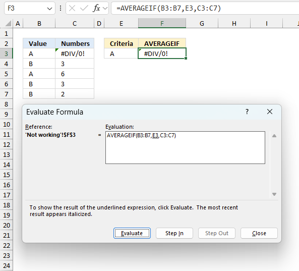
To understand why a formula returns an unexpected value we need to examine the calculations steps in detail. Luckily, Excel has a tool that is really handy in these situations. Here is how to troubleshoot a formula:
- Select the cell containing the formula you want to examine in detail.
- Go to tab “Formulas” on the ribbon.
- Press with left mouse button on "Evaluate Formula" button. A dialog box appears.
The formula appears in a white field inside the dialog box. Underlined expressions are calculations being processed in the next step. The italicized expression is the most recent result. The buttons at the bottom of the dialog box allows you to evaluate the formula in smaller calculations which you control. - Press with left mouse button on the "Evaluate" button located at the bottom of the dialog box to process the underlined expression.
- Repeat pressing the "Evaluate" button until you have seen all calculations step by step. This allows you to examine the formula in greater detail and hopefully find the culprit.
- Press "Close" button to dismiss the dialog box.
There is also another way to debug formulas using the function key F9. F9 is especially useful if you have a feeling that a specific part of the formula is the issue, this makes it faster than the "Evaluate Formula" tool since you don't need to go through all calculations to find the issue..
- Enter Edit mode: Double-press with left mouse button on the cell or press F2 to enter Edit mode for the formula.
- Select part of the formula: Highlight the specific part of the formula you want to evaluate. You can select and evaluate any part of the formula that could work as a standalone formula.
- Press F9: This will calculate and display the result of just that selected portion.
- Evaluate step-by-step: You can select and evaluate different parts of the formula to see intermediate results.
- Check for errors: This allows you to pinpoint which part of a complex formula may be causing an error.
The image above shows cell reference C3:C7 converted to hard-coded value using the F9 key. The AVERAGEIF function requires non-error values which is not the case in this example. We have found what is wrong with the formula.
Tips!
- View actual values: Selecting a cell reference and pressing F9 will show the actual values in those cells.
- Exit safely: Press Esc to exit Edit mode without changing the formula. Don't press Enter, as that would replace the formula part with the calculated value.
- Full recalculation: Pressing F9 outside of Edit mode will recalculate all formulas in the workbook.
Remember to be careful not to accidentally overwrite parts of your formula when using F9. Always exit with Esc rather than Enter to preserve the original formula. However, if you make a mistake overwriting the formula it is not the end of the world. You can “undo” the action by pressing keyboard shortcut keys CTRL + z or pressing the “Undo” button
4.3 Other errors
Floating-point arithmetic may give inaccurate results in Excel - Article
Floating-point errors are usually very small, often beyond the 15th decimal place, and in most cases don't affect calculations significantly.
5. How to use wildcard characters
It is possible to use wildcard characters like (?) question mark or (*) asterisk.
(?) question mark matches any single character.
(*) asterisk matches any sequence of characters even zero charcaters.
Use a tilde (~) before to escape the wildcard characters meaning finding the actual question mark or asterisk.
The following examples demonstrate how to use wildcard characters in the AVERAGEIF function.
6. Begins with

The image above demonstrates how to average corresponding numbers if a value on the same row begins with a specific condition.
Cell range B3:C7 contains the data table, the column header names are "Value" and "Numbers". The condition is specified in cell E3.
Formula in cell F3:
The formula above appends a asterisk character after the condition, this makes the formula match values that begins with the condition. Cells B3 and B6 both begin with the condition specified in cell E3. The corresponding numbers in column C are 8 and 3.
We can now calculate the average. 8+3 = 11. 11 / 2 = 5.5 This number is the same as the number in cell F3. The formula is working as intended.
Explaining formula
Step 1 - Populate arguments
AVERAGEIF(range, criteria, [average_range])
range - B3:B7
criteria - E3&"*"
[average_range] - C3:C7
Step 2 - Evaluate AVERAGEIF function
AVERAGEIF(B3:B7, E3&"*", C3:C7)
becomes
AVERAGEIF({"A-101"; "B-104"; "B-103"; "A-105"; "B-102"}, "A*", {8; 3; 5; 3; 2})
and returns 5.5
8 + 3 = 11
11/2 equals 5.5
7. Ends with

The image above shows a formula in cell F3 that calculates an average if the values in cell range B3:B7 ends with a given condition specified in cell E3.
The corresponding number on the same row in cell range C3:C7 is included in the calculation if the value meets the condition.
Formula in cell F3:
Cells B5 and B7 meet the condition, corresponding cells are C5 and C7. They contain 5 and 2. 5 + 2 equals 7. 7 / 2 equals 3.5
Explaining formula
Step 1 - Populate arguments
AVERAGEIF(range, criteria, [average_range])
range - B3:B7
criteria - "*"&E3
[average_range] - C3:C7
Step 2 - Evaluate AVERAGEIF function
AVERAGEIF(B3:B7, "*"&E3, C3:C7)
becomes
AVERAGEIF({"A-101"; "B-104"; "B-102"; "A-105"; "B-102"}, "*02", {8; 3; 5; 3; 2})
and returns 3.5
5 + 2 = 7
7/2 equals 3.5
8. Contains

This example demonstrates a formula that calculates an average if the corresponding values on the same rows contain a specific condition. In other words, its a partial match meaning the conditions must be found somewhere in the cell value.
The image above shows a data table in cell B3:C7 and the table header names are "Value and Numbers. The condition is specified in cell E3.
Formula in cell F3:
The formula in cell F3 appends asterisks to the beginning and the end of the condition. The ampersand concatenates value to value, the double quotes are used to specify text values in a formula.
Cells B3, and B7 contain the specified condition in cell E3, the numbers on the same rows in column C are 8 and 2. We can now calculate the average: 8 + 2 = 10. 10 / 2 equals 5 which is the same value as in cell F3. The formula in cell F3 works!
Explaining formula
Step 1 - Populate arguments
AVERAGEIF(range, criteria, [average_range])
range - B3:B7
criteria - "*"&E3&"*"
[average_range] - C3:C7
Step 2 - Evaluate AVERAGEIF function
AVERAGEIF(B3:B7, "*"&E3&"*", C3:C7)
becomes
AVERAGEIF({"A-101"; "B-204"; "B-203"; "A-205"; "B-102"}, "*1*", {8; 3; 5; 3; 2})
and returns 5.
8 + 2 = 10
10/2 equals 5
9. Match a specific number of characters

The question mark character ? lets you match any single character in the condition string. The above image demonstrates a formula that uses the following criteria "A-???". In other words, it matches A- and then 3 single characters only.
It matches values in cells B3 and B6. Cell B4 contains a value that almost match, however, it is longer than the requirements. Remember that the question mark only matches a single character.
Formula in cell F3:
The corresponding numbers on the same rows in column C are 8 and 3. 8+3 = 11. 11 / 2 = 5.5 The same value is displayed in cell F3.
Explaining formula
Step 1 - Populate arguments
AVERAGEIF(range, criteria, [average_range])
range - B3:B7
criteria - E3
[average_range] - C3:C7
Step 2 - Evaluate AVERAGEIF function
AVERAGEIF(B3:B7, E3, C3:C7)
becomes
AVERAGEIF({"A-101"; "A-1342"; "AA-802"; "A-205"; "B-102"}, "A-???", {8; 3; 5; 3; 2})
and returns 5.5
8 + 3 = 11
11/2 equals 5.5
10. Is the criteria argument case sensitive?

Does the AVERAGEIF function differentiate between upper and lower letters?
No, the image above shows that the AVERAGEIF function does not consider upper and lower case letters. In other words, the AVERAGEIF function is not case sensitive. The image above shows a data table in cell range B3:C7, it has the following table header names: "Value" and "Numbers".
The condition in cell E3 is uppercase letter "A", however it matches both the lower case letter in cell B6 and the rightly the upper case letter in cell B7. 3+2 = 5. 5/2 = 2.5. This is not what we want. However, the image below describes a workaround. Here is how to:

The image above shows a formula in cell F3 that considers upper and lower cases. In other words it is case sensitive. The data table in cell range B3:C7 has these table header names: Value and Numbers.
The condition in cell E3 is the upper case letter "A". It matches cells B3 and B7 but not cell B6 which contains lower case letter "a".
Array formula in cell F3:
The corresponding numbers in column c are 8 and 2. The average is calculated like this: 8+2 = 10. 10/2 = 5. This value matches the value in cell F3, the formula works!
How to enter an array formula

- Doublepress with left mouse button on cell F3, the prompt appears.
- Type or paste the array formula.
- Press and hold CTRL + SHIFT keys simultaneously.
- Press Enter once.
- Release all keys.
The formula is now entered as an array formula, the formula begins with and ends with a curly bracket, see the image above.
Don't enter these characters yourself, they appear automatically.
Explaining formula
Step 1 - Case sensitive comparison
The EXACT function returns TRUE if two values match also considering upper and lower letters.
EXACT(value1, value2)
EXACT(E3, B3:B7)
becomes
EXACT("A",{"A";"B";"B";"a";"A"})
and returns
{TRUE; FALSE; FALSE; FALSE; TRUE}.
Step 2 - Replace TRUE with corresponding value
The IF function returns one value if the logical test is TRUE and another value if the logical test is FALSE.
IF(logical_test, [value_if_true], [value_if_false])
IF(EXACT(E3, B3:B7), C3:C7, "")
becomes
IF({TRUE; FALSE; FALSE; FALSE; TRUE}, C3:C7, "")
becomes
IF({TRUE; FALSE; FALSE; FALSE; TRUE}, {8; 3; 5; 3; 2}, "")
and returns
{8; ""; ""; ""; 2}.
Step 3 - Calculate average
The AVERAGE function calculates the average of numbers in a cell range.
AVERAGE(number1, [number2], ...)
AVERAGE(IF(EXACT(E3,B3:B7),C3:C7,""))
becomes
AVERAGE({8; ""; ""; ""; 2})
and returns 5.
8 + 2 = 10
10/2 = 5
11. Comparison operators

You are allowed to use the following comparison operators:
- < less than character
- > larger than character
- <> not equal to
- <= less than or equal to
- >= larger than or equal to
The equal sign is never used alone with the value in the criteria argument, the image above shows how to use a condition specified in cell E3 in the AVERAGEIF function.
12. Larger than

This example shows the AVERAGEIF function filtering values larger than a given threshold and calculating the average of the corresponding values on the same row.
The image above shows a data table in cell range B2:C7, it has table header names: "Value" and "Numbers. The condition is specified in cell E3 and is >100.
| Value | Numbers |
| 100 | 5 |
| 105 | 3 |
| 94 | 6 |
| 97 | 3 |
| 102 | 2 |
The formula filters values from column C if the corresponding values in column B are above 100. The greater than sign is a comparison operator that you can use to apply more complicated calculations and filtering.
Formula in cell F3:
Cells B4 and B7 meet the condition, both contain numbers larger than 100, the corresponding numbers in column C on the same row are: 3 and 2. We can now calculate the average by adding the numbers and the divide by the total number of observations.
3 + 2 = 5. 5/2 = 2.5 which is the same as in cell F3. The formula works fine.
Explaining formula
Step 1 - Populate arguments
AVERAGEIF(range, criteria, [average_range])
range - B3:B7
criteria - E3
[average_range] - C3:C7
Step 2 - Evaluate AVERAGEIF function
AVERAGEIF(B3:B7, E3, C3:C7)
becomes
AVERAGEIF({100;105;94;97;102},">100",{5;3;6;3;2})
and returns 2.5
3 + 2 = 5
5/2 equals 2.5
13. Smaller than

This example shows the AVERAGEIF function filtering values smaller than a given threshold and then calculating the average of the corresponding values on the same row.
The image above shows a data table in cell range B2:C7, it has table header names: "Value" and "Numbers. The condition is specified in cell E3 and is <100.
Formula in cell F3:
Cells B5 and B6 meet the condition, both contain numbers smaller than 100, the corresponding numbers in column C on the same row are: 6 and 3. We can now calculate the average by adding the numbers and the divide by the total number of observations.
6 + 3 = 9. 9/2 = 4.5 which is the same as in cell F3. The formula works as intended.
Explaining formula
Step 1 - Populate arguments
AVERAGEIF(range, criteria, [average_range])
range - B3:B7
criteria - E3
[average_range] - C3:C7
Step 2 - Evaluate AVERAGEIF function
AVERAGEIF(B3:B7, E3, C3:C7)
becomes
AVERAGEIF({100;105;94;97;102},"<100",{5;3;6;3;2})
and returns 2.5
6 + 3 = 9
9/2 equals 4.5
14. Not equal to

This example shows the AVERAGEIF function filtering values not equal to a given condition and then calculating the average of the corresponding values on the same row.
The image above shows a data table in cell range B2:C7, it has table header names: "Value" and "Numbers. The condition is specified in cell E3 and is <100.
Formula in cell F3:
Cells B4, B5, B6, and B7 meet the condition, all contain numbers not equal to 100, the corresponding numbers in column C on the same row are: 3, 6, 3, and 2. We can now calculate the average by adding the numbers and the divide by the total number of observations.
3+6+3+2 = 14. 14/4 = 3.5 which is the same as the calculated value in cell F3.
Explaining formula
Step 1 - Populate arguments
AVERAGEIF(range, criteria, [average_range])
range - B3:B7
criteria - E3
[average_range] - C3:C7
Step 2 - Evaluate AVERAGEIF function
AVERAGEIF(B3:B7, E3, C3:C7)
becomes
AVERAGEIF({100;105;94;97;102},"<>100",{5;3;6;3;2})
and returns 2.5
3 + 6 + 3 + 2 = 14
14/4 equals 3.5
'AVERAGEIF' function examples
Functions in 'Statistical' category
The AVERAGEIF function function is one of 73 functions in the 'Statistical' category.
How to comment
How to add a formula to your comment
<code>Insert your formula here.</code>
Convert less than and larger than signs
Use html character entities instead of less than and larger than signs.
< becomes < and > becomes >
How to add VBA code to your comment
[vb 1="vbnet" language=","]
Put your VBA code here.
[/vb]
How to add a picture to your comment:
Upload picture to postimage.org or imgur
Paste image link to your comment.
Contact Oscar
You can contact me through this contact form