How to use the UNIQUE function

What is the UNIQUE function?
The UNIQUE function is a very versatile Excel function, it lets you extract both unique and unique distinct values and also compare columns to columns or rows to rows. It is in the Lookup and reference category and is only available to Excel 365 subscribers.
Table of Contents
1. Syntax
UNIQUE(array,[by_col],[exactly_once])
2. Arguments
| Argument | Text |
| array | Required. Cell range or array. |
| [by_col] | Optional. Boolean value: True or False. True - Compares columns. False (default) - Compares rows. |
| [exactly_once] | Optional. Boolean value: True or False. True - Unique rows or columns False - Unique distinct rows or columns. |
3. Example
Formula in cell D3:
4.0 Unique distinct values

Unique distinct values are all values except that duplicate values are merged into one distinct value.
Formula in cell D3:
The UNIQUE function returns unique distinct values if you only use the first argument with a single-column cell range. The second and third arguments are optional.
Why does the UNIQUE function return a #NAME? error?
First, make sure you spelled the UNIQUE function correctly. If the UNIQUE function still returns a #NAME? error you probably own an earlier Excel version and can't use it unless you upgrade to Excel 365.
There is a small formula you can use if you don't have access to the UNIQUE function, check it out here: How to extract unique distinct values from a column [Formula]
Is the UNIQUE function available for Excel 2003, 2007, 2010, 2013, 2016, and 2019 users?
No, only Excel 365 subscribers have it. However, I made a small formula that works fine, check it out here: How to extract unique distinct values from a column [Formula]
Why does the UNIQUE function return a #SPILL! error?
The UNIQUE function returns an array of values and tries to automatically use the appropriate cell range needed to show all values. If one or more cells are occupied with other values the UNIQUE function returns #SPILL! error.
You have two options, delete or move the values that cause the error or deploy the UNIQUE function in another cell that has adjacent cells below empty.
Why does the UNIQUE function return a #CALC! error?
The UNIQUE function returns a #CALC! error if the output result has no values.
Can I use the UNIQUE function with an Excel Table and structured references?
Yes, you can. The UNIQUE function recalculates the output automatically if you add, edit or delete values in the Excel Table. It works fine with filtered Excel Tables as well.
Is the UNIQUE function case sensitive?
No, it is not case sensitive. Read theses articles if you need a case sensitive formula:
- Extract unique distinct values (case sensitive) [Formula]
- How to extract a case sensitive unique list from a column
4.1 Extract unique distinct values sorted from A to Z

Formula in cell D3:
Check out this article if you own an earlier Excel version and the SORT and UNIQUE functions are not available: Create a unique distinct alphabetically sorted list
Explaining formula in cell D3
Step 1 - Sort values
The SORT function has the following arguments:
SORT(array,[sort_index],[sort_order],[by_col])
The first argument is required, the list is sorted from A to Z if the sort order is omitted.
SORT(B3:B16)
returns
{"Davydenko, Nikolay ";"Del Potro, Juan Martin ";... ;"Verdasco, Fernando "}
Step 2 - Extract unique values
UNIQUE(SORT(B3:B16))
returns {"Davydenko, Nikolay "; "Del Potro, Juan Martin ";... ; "Verdasco, Fernando "}
The UNIQUE function may return an array if more than one value is returned. This will make the formula expand automatically to adjacent cells as far as needed.
How do I return a unique distinct list sorted from Z to A?
Formula in cell D3:
4.2 Extract unique distinct values ignoring blanks

Formula in cell D3:
Check out this article if you own an earlier Excel version and the FILTER and UNIQUE functions are not available: Extract a unique distinct list and ignore blanks
Explaining formula in cell D3
Step 1 - Filter non-empty values
The FILTER function is available for Excel 365 subscribers, it has the following arguments:
FILTER(array,include,[if_empty])
The first argument is the cell range to be filtered, the second argument is the condition or criteria.
FILTER(B3:B16,B3:B16<>"")
returns
{"Federer, Roger ";"Djokovic, Novak "; ... ;"Roddick, Andy "}
Step 2 - Extract unique distinct values
UNIQUE(FILTER(B3:B16,B3:B16<>""))
returns {"Federer, Roger "; "Djokovic, Novak "; ... ; "Verdasco, Fernando "}
4.3 Extract unique distinct values sorted from A to Z ignoring blanks

Formula in cell D3:
Check out this article if you own an earlier Excel version and the FILTER and UNIQUE functions are not available:
Create a unique distinct sorted list containing both numbers text removing blanks
Explaining formula in cell D3
Step 1 - Filter non-empty values
The FILTER function is available for Excel 365 subscribers, it has the following arguments:
FILTER(array,include,[if_empty])
The first argument is the cell range to be filtered, the second argument is the condition or criteria.
FILTER(B3:B16,B3:B16<>"")
returns {"Federer, Roger ";"Djokovic, Novak ";... ;"Roddick, Andy "}
Step 2 - Extract unique distinct values
UNIQUE(FILTER(B3:B16,B3:B16<>""))
returns {"Federer, Roger "; "Djokovic, Novak "; ... ; "Verdasco, Fernando "}
Step 3 - Sort values
The SORT function has the following arguments: SORT(array,[sort_index],[sort_order],[by_col])
The first argument is required, the list is sorted from A to Z if the sort order is omitted.
SORT(UNIQUE(FILTER(B3:B16,B3:B16<>"")))
returns {"Davydenko, Nikolay "; "Del Potro, Juan Martin "; ... ; "Verdasco, Fernando "}
4.4 Count unique distinct values - Excel 365

Formula in cell F3:
The formula above works fine if your cell range doesn't contain any blank cells, the formula below takes care of blanks.
Formula in cell F3:
The ROWS function counts the number of rows that the UNIQUE function returns, that number is how many distinct values there are in cell range B3:B16.
This article explains a formula that works for earlier Excel versions: Count unique distinct values
4.5 Extract unique distinct year and months from dates
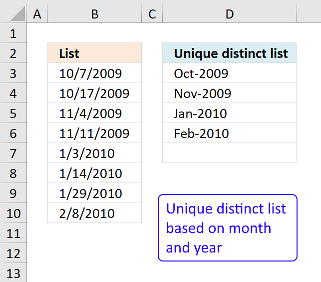
Question: How to create unique distinct year and months from a long date listing (column A)?
You can find the question in this post: Extract dates using a drop down list
4.5.1. Extract unique distinct years and months from dates - Excel 365
Excel 365 dynamic array formula in cell D3:
Explaining formula
Step 1 - Convert dates to given pattern
The TEXT function converts a value to text in a specific number format.
Function syntax: TEXT(value, format_text)
TEXT($B$3:$B$10,"MMM-yyyy")
returns {"Oct-2009"; "Oct-2009"; ... ; "Feb-2010"}
Step 2 - List unique distinct values
The UNIQUE function returns a unique or unique distinct list.
Function syntax: UNIQUE(array,[by_col],[exactly_once])
UNIQUE(TEXT($B$3:$B$10,"MMM-yyyy"))
returns {"Oct-2009"; "Nov-2009"; "Jan-2010"; "Feb-2010"}.
4.5.2. Extract sorted unique distinct years and months based on a list of dates - Excel 365

This formula lists months and years based on dates sorted from newest to oldest, unique distinct means that only one instance of each month and year is displayed.
Explaining formula
Step 1 - Sort dates
The SORT function sorts values from a cell range or array
Function syntax: SORT(array,[sort_index],[sort_order],[by_col])
SORT($B$3:$B$10,,-1) returns {40217; 40207; ... ; 40093}.
Step 2 - Convert dates to given pattern
The TEXT function converts a value to text in a specific number format.
Function syntax: TEXT(value, format_text)
TEXT(SORT($B$3:$B$10,,-1),"MMM-yyyy")
returns {"Feb-2010"; "Jan-2010"; ... ; "Oct-2009"}.
Step 3 - List unique distinct values
The UNIQUE function returns a unique or unique distinct list.
Function syntax: UNIQUE(array,[by_col],[exactly_once])
UNIQUE(TEXT(SORT($B$3:$B$10,,-1),"MMM-yyyy"))
returns {"Feb-2010"; "Jan-2010"; "Nov-2009"; "Oct-2009"}.
4.5.3. Extract unique distinct years and months from dates - earlier Excel versions
Update! 2017-08-23, a smaller easier regular formula:
You can also easily extract a unique distinct list of dates with a pivot table:
Recommended articles
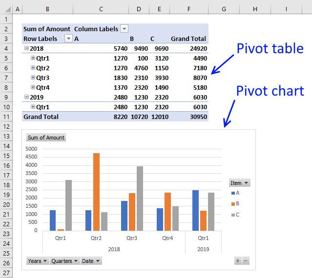
A pivot table allows you to examine data more efficiently, it can summarize large amounts of data very quickly and is very easy to use.
Explaining formula in cell
Step 1 - Convert dates into a given format
The TEXT function lets you convert a value based on a formatting code, in this case we want to convert the date into month and year.
The reason is we want to count previous values against this array to make sure no duplicates show up.
TEXT($B$3:$B$10,"MMM-yyyy") returns {"Oct-2009";"Oct-2009";...; "Feb-2010"}
Step 2 - Count previous values
The COUNTIF function allows us to count values displayed above the current cell using an expanding cell reference.
COUNTIF($D$2:D2,TEXT($B$3:$B$10,"MMM-yyyy"))
returns {0;0;... ;0}
Step 3 - Values represented by a zero has not been displayed yet
COUNTIF($D$2:D2,TEXT($B$3:$B$10,"MMM-yyyy"))=0
returns {TRUE; TRUE; ... ; TRUE}
Step 4 - Divide 1 with array
1/(COUNTIF($D$2:D2,TEXT($B$3:$B$10,"MMM-yyyy"))=0)
returns {1;1;... ;1}
Step 5 - Return date value based on criteria
LOOKUP(2,1/(COUNTIF($D$2:D2,TEXT($B$3:$B$10,"MMM-yyyy"))=0),$B$3:$B$10)
returns 40217.
Step 6 - Convert to month and year
TEXT(LOOKUP(2,1/(COUNTIF($D$2:D2,TEXT($B$3:$B$10,"MMM-yyyy"))=0),$B$3:$B$10),"MMM-yyyy")
returns Feb-2010 in cell D3.
Get *.xlsx file
Extract unique distinct year and months from dates.xlsx
5.0 Unique values

Unique values are values that exist only once in a list. The image above shows a list in column B. Item "AA" has a duplicate and is not unique, however, item "BB" exists only once and is unique.
5.1 Extract unique values

Formula in cell D3:
UNIQUE(array, [by_col], [exactly_once])
The third argument takes logical values True or False. True means unique value, in other words, values that only exist once in the list. False means extracting unique distinct values.
There are only two different values that exist once in cell range B3:B15. All other values have duplicates.
Check out this article if you own an earlier Excel version and the UNIQUE function is not available:
How to filter unique values from a list [Formula]
5.2 Extract unique values sorted from A to Z

Formula in cell D3:
Check out this article if you own an earlier Excel version and the UNIQUE function is not available: Filter unique values sorted from A to Z
Explaining formula in cell D3
Step 1 - Extract unique values
The UNIQUE function has the following arguments:
UNIQUE(array,[by_col],[exactly_once])
UNIQUE(B3:B14,,TRUE)
returns {"Federer, Roger ";"Davydenko, Nikolay ";"Verdasco, Fernando "}
Step 2 - Sort values
The SORT function has the following arguments:
SORT(array,[sort_index],[sort_order],[by_col])
The first argument is required, the list is sorted from A to Z if the sort order is omitted.
SORT(UNIQUE(B3:B14,,TRUE))
returns {"Davydenko, Nikolay "; "Federer, Roger "; "Verdasco, Fernando "}
5.3 Extract unique values ignoring blanks

The UNIQUE function returns 0 (zero) if there is exactly one blank in the list, however, it disappears if there are two or more blanks in the list.
To remove the blank use the following formula.
Formula in cell D3:
Check out this article if you own an earlier Excel version and the UNIQUE function is not available: How to filter unique values from a list [Formula] It works fine with blanks.
Explaining formula in cell D3
Step 1 - Filter non-empty values
The FILTER function is available for Excel 365 subscribers, it has the following arguments:
FILTER(array,include,[if_empty])
The first argument is the cell range to be filtered, the second argument is the condition or criteria.
FILTER(B3:B16,B3:B16<>"")
returns {"Federer, Roger ";"Djokovic, Novak ";... ;"Roddick, Andy "}
Step 2 - Extract unique values
The UNIQUE function has the following arguments:
UNIQUE(array,[by_col],[exactly_once])
UNIQUE(FILTER(B3:B16,B3:B16<>""),,TRUE)
returns {"Federer, Roger ";"Davydenko, Nikolay "}
5.4 Extract unique values sorted from A to Z ignoring blanks

Formula in cell D3:
Check out this article if you own an earlier Excel version and the UNIQUE function is not available: Filter unique values sorted from A to Z It seems to work fine with blanks.
Explaining formula in cell D3
Step 1 - Filter non-empty values
The FILTER function is available for Excel 365 subscribers, it has the following arguments:
FILTER(array,include,[if_empty])
The first argument is the cell range to be filtered, the second argument is the condition or critera.
FILTER(B3:B16,B3:B16<>"") returns {"Federer, Roger ";"Djokovic, Novak ";... ;"Roddick, Andy "}
Step 2 - Extract unique values
The UNIQUE function has the following arguments: UNIQUE(array,[by_col],[exactly_once])
UNIQUE(FILTER(B3:B16,B3:B16<>""),,TRUE) returns {"Federer, Roger ";"Davydenko, Nikolay "}
Step 3 - Sort values
The SORT function has the following arguments:
SORT(array,[sort_index],[sort_order],[by_col])
The first argument is required, the list is sorted from A to Z if the sort order is omitted.
SORT(UNIQUE(FILTER(B3:B16,B3:B16<>""),,TRUE))
returns {"Davydenko, Nikolay"; Federer, Roger "}
6.0 Unique distinct rows

Unique distinct rows are all rows except that duplicate rows are merged to one value.
6.1 Extract unique distinct rows

Formula in cell E3:
Check out this article if you own an earlier Excel version and the UNIQUE function returns a #NAME! error:
Filter unique distinct records
The UNIQUE function recognizes automatically a multicolumn cell range and returns unique distinct rows. The image above shows the UNIQUE function returning three rows, row 4 and 6 are merged into one row.
6.2 Extract unique distinct rows ignoring blank rows

Formula in cell E3:
Check out this article if you own an earlier Excel version and the UNIQUE function returns a #NAME! error:
Filter unique distinct row ignore blanks
Explaining formula in cell E3
Step 1 - Filter non-empty rows
The FILTER function is available for Excel 365 subscribers, it has the following arguments:
FILTER(array, include, [if_empty])
The first argument is the cell range to be filtered, the second argument is the condition or criteria.
FILTER(B3:C6, (C3:C16<>"") * (B3:B6<>"")
returns {"AA", 1; "BB", 2; "AA", 2; "BB", 2}
Step 2 - Extract unique distinct rows
UNIQUE(FILTER(B3:C16,(C3:C16<>"")*(B3:B16<>"")))
returns {"AA", 1; "BB", 2; "AA", 2}
6.3 Extract unique distinct rows sorted from A to Z ignoring blank rows

Formula in cell E3:
This formula sorts the array based on the first column and then on the second column.
Explaining formula in cell E3
Step 1 - Filter non-empty rows
The FILTER function is available for Excel 365 subscribers, it has the following arguments: FILTER(array, include, [if_empty])
The first argument is the cell range to be filtered, the second argument is the condition or criteria.
FILTER(B3:C7, (C3:C7<>"")*(B3:B7<>""))
returns {"AA", 1; "BB", 2; "AA", 2; "BB", 2}
Step 2 - Extract unique distinct rows
UNIQUE(FILTER(B3:C7, (C3:C7<>"")*(B3:B7<>"")))
returns {"AA", 1; "AA", 2; "BB", 2}
Step 3 - Sort array
The SORTBY function lets you sort a multicolumn cell range based on the order of columns you define.
SORTBY(UNIQUE(FILTER(B3:C7, (C3:C7<>"")*(B3:B7<>"")), INDEX(UNIQUE(FILTER(B3:C7, (C3:C7<>"")*(B3:B7<>"")), 0, 1), , INDEX(UNIQUE(FILTER(B3:C7, (C3:C7<>"")*(B3:B7<>"")), 0, 2), )
returns {"AA",1;"AA",2;"BB",2}
Step 4 - Shorten formula
The LET function lets you name an expression that is repeated often in the formula, this allows you to shorten the formula considerably.
SORTBY(UNIQUE(FILTER(B3:C7, (C3:C7<>"")*(B3:B7<>"")), INDEX(UNIQUE(FILTER(B3:C7, (C3:C7<>"")*(B3:B7<>"")), 0, 1), , INDEX(UNIQUE(FILTER(B3:C7, (C3:C7<>"")*(B3:B7<>"")), 0, 2), )
x - UNIQUE(FILTER(B3:C7, (C3:C7<>"")*(B3:B7<>"")), FALSE)
LET(x, UNIQUE(FILTER(B3:C7, (C3:C7<>"")*(B3:B7<>"")), FALSE), SORTBY(x, INDEX(x, 0, 1), , INDEX(x, 0, 2), ))
7.0 Unique rows

Unique rows are rows that exist only once in a cell range. The image above shows that B4:C4 and B6:D6 are duplicates and are not in the result in cell range E3:F4.
7.1 Extract unique rows

Formula in cell E3:
The third argument in the UNIQUE function determines if rows that exist exactly once should be extracted.
UNIQUE(array,[by_col],[exactly_once]) Default is False. The formula above is entered as a regular formula.
The following array formula works for older Excel versions than Excel 365.
Array formula in cell E3:
How to enter an array formula
These steps are for earlier Excel versions.
- Copy the above array formula.
- Double-press with left mouse button on cell E3.
- Paste array formula.
- Press and hold CTRL + SHIFT simultaneously.
- Press Enter.
- Release all keys.
7.2 Extract unique rows ignoring blank rows

Formula in cell E3:
The formula above is entered as a regular formula.
The following array formula works for older Excel versions than Excel 365.
Array formula in cell E3:
How to enter an array formula
- Copy the above array formula.
- Double-press with left mouse button on cell E3.
- PAste array formula.
- Press and hold CTRL + SHIFT simultaneously.
- Press Enter.
- Release all keys.
Explaining Excel 365 formula in cell E3
Step 1 - Filter non-empty values
The FILTER function is available for Excel 365 subscribers, it has the following arguments:
FILTER(array, include, [if_empty])
The first argument is the cell range to be filtered, the second argument is the condition or criteria.
FILTER(B3:C8,(C3:C8<>"")*(B3:B8<>""))
returns {"AA", 1; "BB", 2; "AA", 2; "BB", 2}
Step 2 - Extract unique rows
The third argument in the UNIQUE function determines if rows that exist exactly once should be extracted.
UNIQUE(array,[by_col],[exactly_once]) Default is False meaning distinct values (not unique).
UNIQUE(FILTER(B3:C8, (C3:C8<>"")*(B3:B8<>"")), FALSE, TRUE)
returns {"AA", 1; "AA", 2}
7.3 Extract unique rows sorted from A to Z ignoring blank rows

This formula sorts the data set based on the first column (B) and the on the second column (C).
Formula in cell E3:
The formula above is entered as a regular formula.
Explaining formula in cell E3
Step 1 - Filter non-empty values
The FILTER function is available for Excel 365 subscribers, it has the following arguments:
FILTER(array, include, [if_empty])
The first argument is the cell range to be filtered, the second argument is the condition or criteria.
FILTER(B3:C8, (C3:C8<>"")*(B3:B8<>""))
returns {"AA", 2; "BB", 2; "AA", 1; "BB", 2}
Step 2 - Extract unique rows
The third argument in the UNIQUE function determines if rows that exist exactly once should be extracted.
UNIQUE(array,[by_col],[exactly_once]) Default is False meaning distinct values (not unique).
UNIQUE(FILTER(B3:C8, (C3:C8<>"")*(B3:B8<>"")), , TRUE)
returns {"AA", 2; "AA", 1}
Step 3 - Sort array
The SORTBY function lets you sort a multicolumn cell range based on the order of columns you define.
SORTBY(array, by_array1, [sort_order1], [by_array2, sort_order2],…)
SORTBY(UNIQUE(FILTER(B3:C8, (C3:C8<>"")*(B3:B8<>"")), , TRUE), INDEX(UNIQUE(FILTER(B3:C8, (C3:C8<>"")*(B3:B8<>"")), , TRUE), 0, 1), , INDEX(UNIQUE(FILTER(B3:C8, (C3:C8<>"")*(B3:B8<>"")), , TRUE), 0, 2), )
returns {"AA", 1; "AA", 2}
Step 4 - Shrink formula
The LET function lets you name an expression that is repeated often in the formula, this allows you to shorten the formula considerably.
SORTBY(UNIQUE(FILTER(B3:C8, (C3:C8<>"")*(B3:B8<>"")), , TRUE), INDEX(UNIQUE(FILTER(B3:C8, (C3:C8<>"")*(B3:B8<>"")), , TRUE), 0, 1), , INDEX(UNIQUE(FILTER(B3:C8, (C3:C8<>"")*(B3:B8<>"")), , TRUE), 0, 2), )
This part: UNIQUE(FILTER(B3:C8, (C3:C8<>"")*(B3:B8<>"")), , TRUE) is repeated three times in the formula.
x - UNIQUE(FILTER(B3:C8, (C3:C8<>"")*(B3:B8<>"")), , TRUE)
LET(x, UNIQUE(FILTER(B3:C8, (C3:C8<>"")*(B3:B8<>"")), , TRUE), SORTBY(x, INDEX(x, 0, 1), , INDEX(x, 0, 2), ))
8.0 Unique and unique distinct columns

8.1 Extract unique distinct columns

Formula in cell E3:
The formula above is entered as a regular formula.
8.2 Extract unique columns

Formula in cell E3:
The formula above is entered as a regular formula.
Useful links
10. Remove duplicates based on date
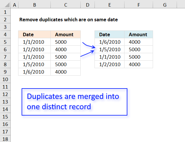
This example demonstrates a formula for Excel versions that don't have the UNIQUE function. If you have the UNIQUE function then use this formula in cell E5:
Question:
Column B has dates Column C as data
B5 : 1/1/2010 : 5000
B6 : 2/1/2010 : 4000
B7 : 1/1/2010 : 5000
B8 : 5/1/2010 : 5000
B9 : 6/1/2010 : 4000
From column C the values which are duplicate i want to remove only those which are on same date .
Remove Duplicates from Column C by comparing from Column B Which has date. as, if the duplication is occurred on next date it should not be counted as not a duplicate because the same data is entered in the next date.
Example : Customer has Purchased Item A on 1/1/2010
Customer has purchase Item A on 1/1/2010
I want to assume that On 1/1/2010 Item A has a duplicate
If the customer has purchased Item A on 2/1/2010 . this is not duplicate because the item is purchased on the next date.
Answer:
Array formula in E5:
Explaining formula in cell E5
Step 1 - Prevent duplicate records
The COUNTIFS function counts the number of cells across multiple ranges that equals all given conditions.
Every other argument in the COUNTIFS function contains an expanding cell reference, when the cell is copied to cells below the cell references grows accordingly. This makes the formula aware of previously shown values which prevents duplicates from showing up.
COUNTIFS($E$4:$E4, $B$5:$B$9, $F$4:$F4, $C$5:$C$9)=0
returns {TRUE; TRUE; ... ; TRUE}.
Step 2 - Divide 1 with array
If the array contains an error the LOOKUP function will ignore it which is great. To create an error for values that are FALSE (equivalent to 0 zero) simply divide 1 with the array.
1/(COUNTIFS($E$4:$E4, $B$5:$B$9, $F$4:$F4, $C$5:$C$9)=0)
returns {1;1;1;1;1}.
Step 3 - Get value
LOOKUP(2, 1/(COUNTIFS($E$4:$E4, $B$5:$B$9, $F$4:$F4, $C$5:$C$9)=0), B$5:B$9)
returns 40184 (1/6/2010) in cell E5.
Get Excel *.xlsx file
remove dupes on same date.xlsx
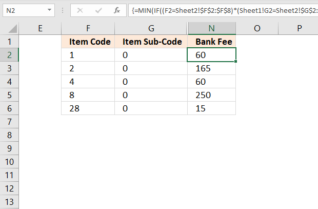
11. How to create a unique distinct list based on two conditions

Question: How do I create a unique distinct list where other columns meet two criteria using excel array formula?
Answer:
Excel 365 dynamic formula in cell I3:
Excel 2007 array formula in H2:
How to create an array formula
- Copy (Ctrl + c) and paste (Ctrl + v) array formula into formula bar.
- Press and hold Ctrl + Shift.
- Press Enter once.
- Release all keys.
Copy cell H2. Paste down to cell H16.
Earlier Excel versions, array formula in H2:
Copy cell H2. Paste down to cell H16.
Explaining excel 2007 array formula in cell H2
Step 1 - Create boolean array with values indicating unique distinct values
=IFERROR(INDEX(List, MATCH(0, COUNTIF(H1:$H$1, List)+IF(Category2<>Criteria2, 1, 0)+IF(Category1<>Criteria1, 1, 0), 0)), "")
COUNTIF(H1:$H$1, List)
returns {0; 0; 0; 0; 0; 0; 0; 0; 0; 0; 0; 0; 0; 0; 0}.
Recommended articles

Counts the number of cells that meet a specific condition.
Step 2 - Create boolean array with values indicating first criterion
=IFERROR(INDEX(List, MATCH(0, COUNTIF(H1:$H$1, List)+IF(Category2<>Criteria2, 1, 0)+IF(Category1<>Criteria1, 1, 0), 0)), "")
IF(Category1<>Criteria1, 1, 0) returns {0;1;... ;0}.
Recommended articles
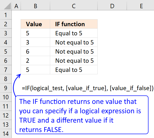
Checks if a logical expression is met. Returns a specific value if TRUE and another specific value if FALSE.
Step 3 - Create boolean array with values indicating second criterion
=IFERROR(INDEX(List, MATCH(0, COUNTIF(H1:$H$1, List)+IF(Category2<>Criteria2, 1, 0)+IF(Category1<>Criteria1, 1, 0), 0)), "")
IF(Category2<>Criteria2, 1, 0) returns {0; 1; ... ; 1}.
Step 4 - Add boolean arrays
=IFERROR(INDEX(List, MATCH(0, COUNTIF(H1:$H$1, List)+IF(Category2<>Criteria2, 1, 0)+IF(Category1<>Criteria1, 1, 0), 0)), "")
becomes
=IFERROR(INDEX(List, MATCH(0,{0;2;1;1;0;1;0;1;1;1;0;1;1;1;1}, 0)), "")
Step 4 - Return relative position of the first zero (0) in array
=IFERROR(INDEX(List, MATCH(0,{0;2;1;1;0;1;0;1;1;1;0;1;1;1;1}, 0)), "")
becomes
=IFERROR(INDEX(List, 1), "")
Recommended articles
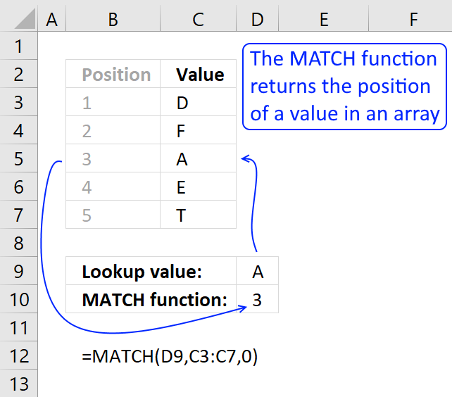
Identify the position of a value in an array.
Step 5 - Return a value or reference of the cell at the intersection of a particular row and column
=IFERROR(INDEX(List, 1), "")
becomes
=IFERROR(4, "")
Recommended articles
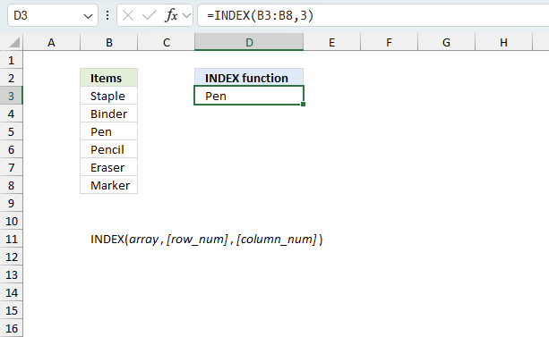
Gets a value in a specific cell range based on a row and column number.
Step 6 - Check if expression returns an error
=IFERROR(4, "")
returns number 4 in cell H2.
Recommended articles
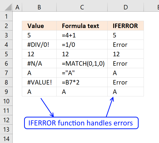
The IFERROR function lets you catch most errors in Excel formulas. It was introduced in Excel 2007. In previous Excel […]
Get excel file.
create-a-list-of-distinct-values-from-two-criteria.xlsx
(Excel 2007 Workbook *.xlsx)
create-a-list-of-distinct-values-from-two-criteria.xls
(Excel 97-2003 Workbook *.xls)
Explaining excel 2007 array formula in cell H2
Step 1 - Create boolean array with values indicating unique distinct values
=IFERROR(INDEX(List, MATCH(0, COUNTIF(H1:$H$1, List)+IF(Category2<>Criteria2, 1, 0)+IF(Category1<>Criteria1, 1, 0), 0)), "")
COUNTIF(H1:$H$1, List) returns {0; ... ; 0}.
Recommended articles
Counts the number of cells that meet a specific condition.
Step 2 - Create boolean array with values indicating first criterion
=IFERROR(INDEX(List, MATCH(0, COUNTIF(H1:$H$1, List)+IF(Category2<>Criteria2, 1, 0)+IF(Category1<>Criteria1, 1, 0), 0)), "")
IF(Category1<>Criteria1, 1, 0) returns {0;1;... ;0}.
Recommended articles
Checks if a logical expression is met. Returns a specific value if TRUE and another specific value if FALSE.
Step 3 - Create boolean array with values indicating second criterion
=IFERROR(INDEX(List, MATCH(0, COUNTIF(H1:$H$1, List)+IF(Category2<>Criteria2, 1, 0)+IF(Category1<>Criteria1, 1, 0), 0)), "")
IF(Category2<>Criteria2, 1, 0) returns {0; ... ; 1}.
Step 4 - Add boolean arrays
IFERROR(INDEX(List, MATCH(0, COUNTIF(H1:$H$1, List)+IF(Category2<>Criteria2, 1, 0)+IF(Category1<>Criteria1, 1, 0), 0)), "")
IFERROR(INDEX(List, MATCH(0,{0;2;1;1;0;1;0;1;1;1;0;1;1;1;1}, 0)), "")
Step 4 - Return relative position of the first zero (0) in array
=IFERROR(INDEX(List, MATCH(0,{0;2;1;1;0;1;0;1;1;1;0;1;1;1;1}, 0)), "")
becomes
IFERROR(INDEX(List, 1), "")
Recommended articles
Identify the position of a value in an array.
Step 5 - Return a value or reference of the cell at the intersection of a particular row and column
=IFERROR(INDEX(List, 1), "")
becomes
IFERROR(4, "")
Recommended articles
Gets a value in a specific cell range based on a row and column number.
Step 6 - Check if expression returns an error
IFERROR(4, "")
returns number 4 in cell H2.
Recommended articles
The IFERROR function lets you catch most errors in Excel formulas. It was introduced in Excel 2007. In previous Excel […]
Get excel file.
create-a-list-of-distinct-values-from-two-criteria.xlsx
(Excel 2007 Workbook *.xlsx)
create-a-list-of-distinct-values-from-two-criteria.xls
(Excel 97-2003 Workbook *.xls)
12. Function not working
The UNIQUE function
- returns #NAME? error if you misspell the function name.
- propagates errors, meaning that if the input contains an error (e.g., #VALUE!, #REF!), the function will return the same error.
12.1 Troubleshooting the error value
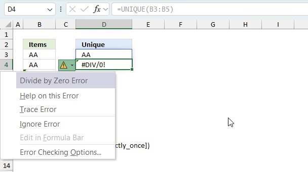
When you encounter an error value in a cell a warning symbol appears, displayed in the image above. Press with mouse on it to see a pop-up menu that lets you get more information about the error.
- The first line describes the error if you press with left mouse button on it.
- The second line opens a pane that explains the error in greater detail.
- The third line takes you to the "Evaluate Formula" tool, a dialog box appears allowing you to examine the formula in greater detail.
- This line lets you ignore the error value meaning the warning icon disappears, however, the error is still in the cell.
- The fifth line lets you edit the formula in the Formula bar.
- The sixth line opens the Excel settings so you can adjust the Error Checking Options.
Here are a few of the most common Excel errors you may encounter.
#NULL error - This error occurs most often if you by mistake use a space character in a formula where it shouldn't be. Excel interprets a space character as an intersection operator. If the ranges don't intersect an #NULL error is returned. The #NULL! error occurs when a formula attempts to calculate the intersection of two ranges that do not actually intersect. This can happen when the wrong range operator is used in the formula, or when the intersection operator (represented by a space character) is used between two ranges that do not overlap. To fix this error double check that the ranges referenced in the formula that use the intersection operator actually have cells in common.
#SPILL error - The #SPILL! error occurs only in version Excel 365 and is caused by a dynamic array being to large, meaning there are cells below and/or to the right that are not empty. This prevents the dynamic array formula expanding into new empty cells.
#DIV/0 error - This error happens if you try to divide a number by 0 (zero) or a value that equates to zero which is not possible mathematically.
#VALUE error - The #VALUE error occurs when a formula has a value that is of the wrong data type. Such as text where a number is expected or when dates are evaluated as text.
#REF error - The #REF error happens when a cell reference is invalid. This can happen if a cell is deleted that is referenced by a formula.
#NAME error - The #NAME error happens if you misspelled a function or a named range.
#NUM error - The #NUM error shows up when you try to use invalid numeric values in formulas, like square root of a negative number.
#N/A error - The #N/A error happens when a value is not available for a formula or found in a given cell range, for example in the VLOOKUP or MATCH functions.
#GETTING_DATA error - The #GETTING_DATA error shows while external sources are loading, this can indicate a delay in fetching the data or that the external source is unavailable right now.
12.2 The formula returns an unexpected value
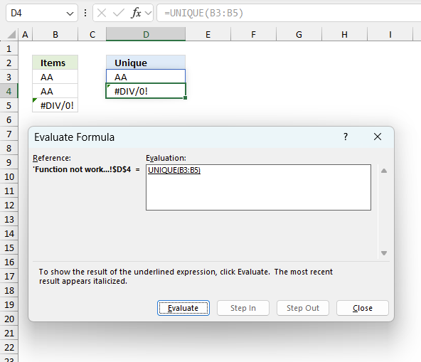
To understand why a formula returns an unexpected value we need to examine the calculations steps in detail. Luckily, Excel has a tool that is really handy in these situations. Here is how to troubleshoot a formula:
- Select the cell containing the formula you want to examine in detail.
- Go to tab “Formulas” on the ribbon.
- Press with left mouse button on "Evaluate Formula" button. A dialog box appears.
The formula appears in a white field inside the dialog box. Underlined expressions are calculations being processed in the next step. The italicized expression is the most recent result. The buttons at the bottom of the dialog box allows you to evaluate the formula in smaller calculations which you control. - Press with left mouse button on the "Evaluate" button located at the bottom of the dialog box to process the underlined expression.
- Repeat pressing the "Evaluate" button until you have seen all calculations step by step. This allows you to examine the formula in greater detail and hopefully find the culprit.
- Press "Close" button to dismiss the dialog box.
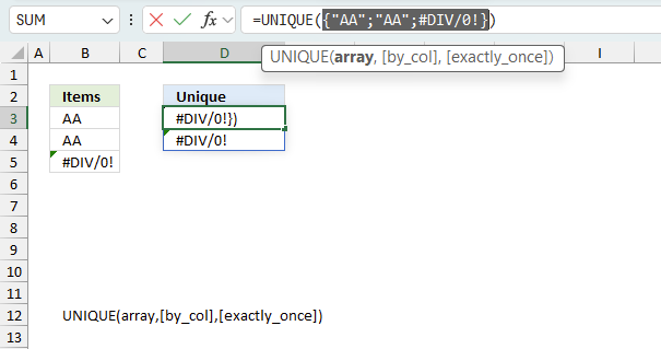
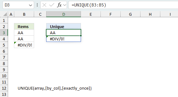
There is also another way to debug formulas using the function key F9. F9 is especially useful if you have a feeling that a specific part of the formula is the issue, this makes it faster than the "Evaluate Formula" tool since you don't need to go through all calculations to find the issue..
- Enter Edit mode: Double-press with left mouse button on the cell or press F2 to enter Edit mode for the formula.
- Select part of the formula: Highlight the specific part of the formula you want to evaluate. You can select and evaluate any part of the formula that could work as a standalone formula.
- Press F9: This will calculate and display the result of just that selected portion.
- Evaluate step-by-step: You can select and evaluate different parts of the formula to see intermediate results.
- Check for errors: This allows you to pinpoint which part of a complex formula may be causing an error.
The image above shows cell reference B3:B5 converted to hard-coded value using the F9 key. The UNIQUE function requires non-error values which is not the case in this example. We have found what is wrong with the formula.
Tips!
- View actual values: Selecting a cell reference and pressing F9 will show the actual values in those cells.
- Exit safely: Press Esc to exit Edit mode without changing the formula. Don't press Enter, as that would replace the formula part with the calculated value.
- Full recalculation: Pressing F9 outside of Edit mode will recalculate all formulas in the workbook.
Remember to be careful not to accidentally overwrite parts of your formula when using F9. Always exit with Esc rather than Enter to preserve the original formula. However, if you make a mistake overwriting the formula it is not the end of the world. You can “undo” the action by pressing keyboard shortcut keys CTRL + z or pressing the “Undo” button
12.3 Other errors
Floating-point arithmetic may give inaccurate results in Excel - Article
Floating-point errors are usually very small, often beyond the 15th decimal place, and in most cases don't affect calculations significantly.
'UNIQUE' function examples

First, let me explain the difference between unique values and unique distinct values, it is important you know the difference […]
This article describes an array formula that compares values from two different columns in two worksheets twice and returns a […]
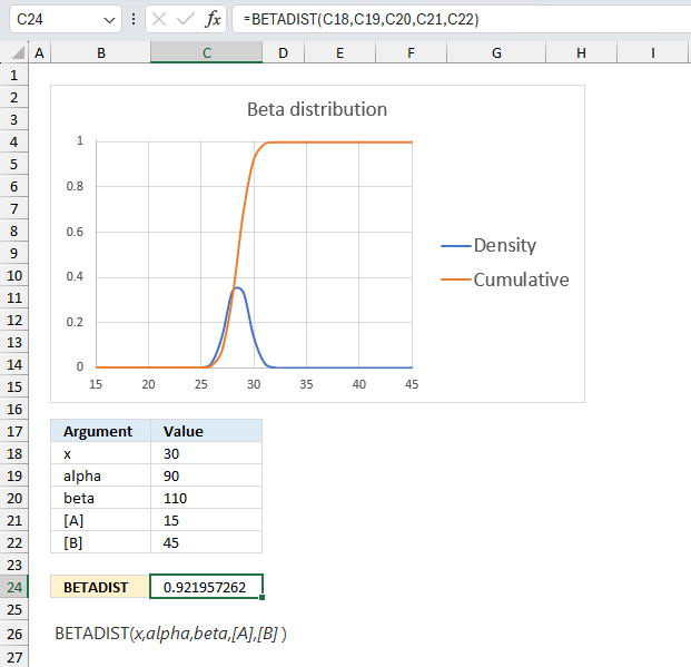
Table of Contents How to use the BETADIST function How to use the BETAINV function How to use the BINOMDIST […]
Functions in 'Lookup and reference' category
The UNIQUE function function is one of 25 functions in the 'Lookup and reference' category.
Excel function categories
Excel categories
35 Responses to “How to use the UNIQUE function”
Leave a Reply
How to comment
How to add a formula to your comment
<code>Insert your formula here.</code>
Convert less than and larger than signs
Use html character entities instead of less than and larger than signs.
< becomes < and > becomes >
How to add VBA code to your comment
[vb 1="vbnet" language=","]
Put your VBA code here.
[/vb]
How to add a picture to your comment:
Upload picture to postimage.org or imgur
Paste image link to your comment.
[...] in Excel on Apr.13, 2010. Email This article to a Friend In a previous post we created a unique distinct list of dates and data removing any duplicates on same [...]
your array formula examples are fantastic and incredibly useful, thank you! this one provides almost all the insight I need, except for sorting the result list. I've tried to apply the sorting techniques from some of your other examples and am just not getting it. Can you help?
well after a few hours I think I've figured it out, just need to handle blank rows.
{=IFERROR(INDEX(tbl2,SMALL(IF(SMALL(IF(((($F$2=Color)*($G$2=Texture)*(COUNTIF($I$1:I1,tbl2)=0))),COUNTIF(tbl2,"<"&tbl2)+1,""),1)=COUNTIF(tbl2,"<"&tbl2)+1,ROW(tbl2)-MIN(ROW(tbl2))+1),1)),"")}
where
tbl2 = the original list
'Color' is a range defined on a column next to tbl2, specifying a color for each entry. The same for 'Texture.'
F2 and G2 define the color and texture to be selected, and "I" defines the output column.
Congratulations!
You did it!
Thank you for your contribution!
I modified your named ranges for this post.
Array formula in H2:
=IFERROR(INDEX(List, SMALL(IF(SMALL(IF(((($F$2=Category2)*($F$1=Category1)*(COUNTIF($H$1:H1, List)=0))), COUNTIF(List, "<"&List)+1, ""), 1)=COUNTIF(List, "<"&List)+1, ROW(List)-MIN(ROW(List))+1), 1)), "") + CTRL + SHIFT + ENTER copied down as far as needed.
Oscar this site's been a great help. Having a problem with the above formula for earlier versions though. Should there be semicolons in it?
Andy Green,
Thanks!
No, I have removed the semicolons.
Thanks Oscar. Still getting "Too many arguments for this function.
Thinking about it, it may help if I tell you exactly what I'm trying to do. I'm trying to extract a list of unique values, based on a number of criteria, including some "OR's". Any ideas. I can normally find everything on here but this has me stumped
Andy Green,
It works now, get the attached xls file or copy array formula.
Thanks for letting me know!
Oscar you're a star. You're gonna love me for this....How would I add an "OR" in there. ie Say there was a row such as....
BB C 7
As there's already a Category2"B" I can't add a "+IF(Category2"C", 1, 0)"
So how would I include that one? Any ideas or am I just pushing my luck?
Andy Green,
Named ranges
List (C2:C16)
Category1 (A2:A16)
Category2 (B2:B16)
Criteria1 (F1)
Criteria2 (F2:F3)
Excel 2007 array formula in H2:
Earlier Excel versions, array formula in H2:
You are the Excel Joda!
Yoda quote:
"Feel the (excel) force!"
[...] tables to the web >> Excel Jeanie HTML 4 You can find the above formulas here..... How to create a unique distinct list where other columns meet two criteria | Get Digital Help - Micr... Count unique distinct records with a date and column criteria in excel 2007 | Get Digital Help - [...]
I've solved a similar problem inverting the results (1 and 0) of the "IF" clauses. I post it here in case someone would find it useful:
=INDEX(List; MATCH(0; COUNTIF($H$1:H1; List) + IF(Category>0;0;1) + IF(Category0 and <2)
Hi,
This is absolutely great and it's what I need. I do have one question and maybe it might be the operator (me). I opened the attached file the xlsx version of the file and when I go into the formula to change the range for my data and go out of the cell it returns a blank. If I take out the IFERROR statement it shows a #N/A. I don't understand what I'm doing wrong. Can you help?
Thanks,
Sorry me again. It's the operator with the issue. I didn't change it back to an array formula.
Hi,
Is there a way to make this work on ranges? like, if a cell is larger than 3 and smaller than 5.
I'm sorry, I figured it out now.
I just replaced it with a ">" and "<" so it turns out FALSE and it worked.
Thanks for the code :)
Is there a way to do this without using the IFERROR? The speed of my workbook has ground to a halt after doing this formula. I have 1800 rows of data. Thanks in advance!
I have 4K rows - does it break if there are too many rows - it seems to stop functioning for me.
Jackie,
I recommend using formulas as described in the post if you need a "dynamic" calculation like in a dashboard or similar.
Follow instructions below if you want to simply remove duplicate records.
Select cell range A1:B5.
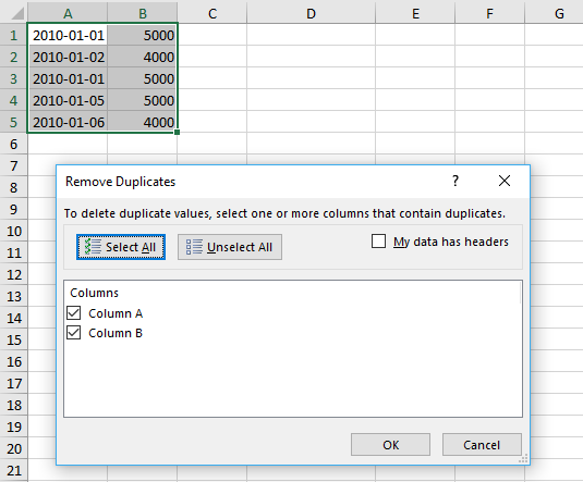
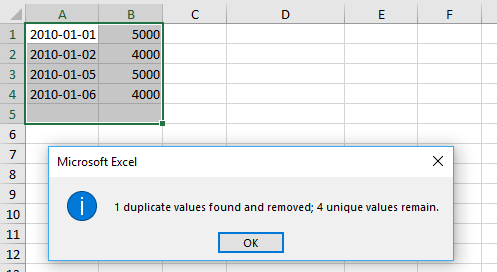
Go to tab "Data" on the ribbon.
Press with left mouse button on "Remove Duplicates" button
Press with left mouse button on OK
Press with left mouse button on OK button
How to Get in Sorted Order (ASC or DESC)?
Thanks!
Qadeer Ahmed,
Great question. Formula in cell D2:
ASC
=TEXT(SMALL(IF(COUNTIF($D$1:D1, TEXT($A$2:$A$135, "mmm-YYYY")), "", $A$2:$A$135), ROWS($A$1:A1)), "mmm-YYYY")
DESC
=TEXT(LARGE(IF(COUNTIF($D$1:D1, TEXT($A$2:$A$135, "mmm-YYYY")), "", $A$2:$A$135), ROWS($A$1:A1)), "mmm-YYYY")
Thanks for helping Oscar, it works! :)
Not working for me.
The Excel file sorts from top to bottom in descending order.
The solution Oscar gave is giving errors.
Please help.
Brandon,
You need to adjust the bolded cell range to the cell above your selected cell.
=TEXT(SMALL(IF(COUNTIF($D$1:D1, TEXT($A$2:$A$135, "mmm-YYYY")), "", $A$2:$A$135), ROWS($A$1:A1)), "mmm-YYYY")
Did that help?
Hi, Do you have any idea to show all unique values in one cell
Saravana Kumar,
Yes, this formula works in Excel 365. It is based on the example in this article.
I have a typical query. Given in sequence
1. I have one unique ID for VLOOKUP.
2. Against this Unique ID, there are multiple IDs available and multiple values in text.
3. For example, Unique ID 123456 (Customer Code), there are one more terminals provided with different Merchant ID. Out of this Merchant ID under a single Unique ID, there are various values available like "Approved", "Active", "Hotlisted".
4. Now for a single Unique ID, as explained in 3 above, there are multiple values.
5. I need to consolidate the above with a formula. How to go about and what are the formulae to adopt.
Thank you.
Hello Yoda,
is it possible to have this formula with 3 criteria? i tried but... :)
=TEXT(SMALL(IF(COUNTIF($D$1:D1, TEXT($A$2:$A$135, "mmm-YYYY")), "", $A$2:$A$135), ROWS($A$1:A1)), "mmm-YYYY")
This formula is only working partially for me with errors.
Wouldn't a simpler formula be:
=UNIQUE(TEXT($B$3:$B$10,"MMM-yyyy"))
Stuart,
yes, Excel 365 has great new functions.