How to use the RANDBETWEEN function

What is the RANDBETWEEN function?
It returns a random whole number between the numbers you specify. This function is volatile meaning a new random number is created every time the worksheet is calculated.
Table of Contents
- Introduction
- Syntax
- Example 1
- Example 2
- Example 3
- Random numbers with a decimal
- Random negative numbers with two decimals
- Random negative numbers with three decimals
- Random names
- Random list
- Create random text strings
- Random numbers
- Random text strings
- Random date values
- Random time values
- Assign records unique random text strings
- Function not working
1. Introduction
What is random?
Each outcome of a random process cannot be predicted with certainty before it occurs. It is unpredictable.
Is the RANDBETWEEN function random?
No, it is pseudo-random. The generated value is not truly random.
What is pseudo-random?
True randomness doesn't really exist in software like Excel. The random values only look random, but are not actually random since they come from an algorithm.
What is volatile?
The RANDBETWEEN function is volatile, which means that every time the worksheet recalculates, the function runs again and a new random-looking number is returned.
What is the effect of volatile functions?
Having a lot of volatile random functions like RANDBETWEEN on your worksheet can slow down calculation, because they keep recalculating even when their inputs don't change.
When is the worksheet calculated?
Cells containing non volatile functions are only calculated once or until you force a recalculation, however, volatile functions are recalculated each time you type in a cell and press enter.
Can you stop recalculating a worksheet?
Yes, you can change a setting to manual recalculations.
- Go to tab "Formulas".
- Press with left mouse button on the "Calculation Options" button, a popup menu appears.
- Press with mouse on "Manual".
This stops the automatic recalculations.
How to force a recalculation?
Pressing F9 key will recalculate or refresh all the formulas and values in every worksheet of every workbook you have open.
Pressing Shift+F9 will only recalculate the formulas and values on the single worksheet you're currently viewing or active.
Pressing Ctrl+Alt+F9 is the quickest way to force a full recalculation of absolutely everything in all open workbooks, even if nothing has changed. It ignores whether changes were made or not and completely recomputes.
Are there more volatile functions in Excel?
Yes. OFFSET, TODAY, NOW among others.
| Function | Syntax | Description |
|---|---|---|
| OFFSET | OFFSET(reference, rows, cols) | Returns a cell offset from a reference cell. |
| TODAY | TODAY() | Returns the current date. |
| NOW | NOW() | Returns current date and time. |
| RANDARRAY | RANDARRAY([rows], [columns], [min], [max], [whole_number]) | Returns an array with random numbers. |
| RANDBETWEEN | RANDBETWEEN(bottom, top) | Returns a random whole number between bottom and top |
Note, that conditional formatting is extremely volatile or super-volatile meaning it is recalculated as you scroll through a worksheet.
What other functions return random values?
| Excel Function | Syntax | Description |
|---|---|---|
| RAND() | RAND() | Returns a random decimal number between 0 and 1 |
| RANDBETWEEN | RANDBETWEEN(bottom, top) | Returns a random whole number between bottom and top |
| RANDARRAY | RANDARRAY([rows], [columns], [min], [max], [whole_number]) | Returns an array with random numbers. |
Formula in cell D3:
2. Syntax
RANDBETWEEN(bottom, top)
| bottom | Required. The start number of the range you want to create a random number from. |
| top | Required. The end number of the range you want to create a random number from. |
Press F9 to calculate new random numbers. Use this function with care, it may slow down your workbook considerably if used extensively. This is the case with all volatile functions.
3. Example 1
This example demonstrates how to use the RANDBETWEEN function. It has two arguments bottom and top, which determines the range or boundary the RANDBETTWEEN function can output whole numbers from.
The image above has the bottom value in cell B4 and it contains 5, the top value in cell C4 and it contains 54. The function is in cell B7 and it returns 21 in this example.
Formula in cell B7:
The output value 21 which is displayed in cell B7 is larger then the bottom value specified in cell B4 and smaller than the top value specified in cell C4. The function is volatile meaning the output value changes each time the worksheet is recalculated which happens each time you enter a new value and presses Enter.
4. Example 2

This example demonstrates how to create a right triangle based on random coordinates created by the RANDBETWEEN function. The graph shown in the image above has minimum value of -10 and a maximum value of 10 which are valid for both the x axis and y axis.
The triangle in the chart is created from these two random whole numbers in cells C19 and C20.
Formula in cell C19:
Formula in cell C20:
Cell C19 creates a random whole number between -10 and 10 which is the used in cells B24, B26, B27, and B29 to create the x axis values for the right triangle displayed in the chart above.
The y axis value is created in cell C20 between -10 and 10 which is then used in cells B27 and B29. These values are needed to create the triangle displayed in the chart above.
You can press function key F9 to generate a new triangle with new random x and y values. The chart is instantly updated based on the new values.
5. Example 3

This example demonstrates a formula that picks a random named from cell range B4:B14. Press function key F9 to generate a new random name.
Formula in cell D4:
This example displays "Ted" in cell D4 which is in cell B11 in the source data. Here is how the formula works:
- Create a random whole number between 1 and 11.
- Return the corresponding value from cell range B4:B14. There are 11 cells in cell range B4:B14
The following sections explains the formula in greater detail.
Explaining the formula in cell D4
Step 1 - Generate a random value between 1 and 11
The RANDBETWEEN function has the following arguments: bottom and top
The bottom value is 1 and the top value is 11.
RANDBETWEEN(1,11) which returns 8 in the example shown in the image above.
Step 2 - Get value from B4:B14 based on random whole number
The INDEX function returns a value or reference from a cell range or array, you specify which value based on a row and column number.
Function syntax: INDEX(array, [row_num], [column_num])
INDEX(B4:B14, RANDBETWEEN(1,11)) becomes INDEX(B4:B14, 8)
and returns "Ted". The eighth cell in B4:B14 is B11 and it contains name "Ted".
6. Random numbers
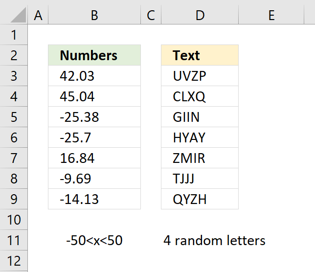
Microsoft Excel has three useful functions for generating random numbers, the RAND, RANDBETWEEN, and the RANDARRAY functions.
The RAND function returns a random decimal number equal to or larger than 0 (zero) and smaller than 1. Example: 0.600842025092928
The RANDARRAY function calculates an array of random numbers. It allows you to choose integers or decimal values, how many rows and columns to fill and the number range.
This is a new function available for Excel 365 subscribers in the monthly channel, it automatically spills values across rows and columns without the need to enter it as an array formula. This is called spilled array behavior and is a new feature in Excel.
RANDBETWEEN function returns random integers in a range you specify. The function has two arguments: bottom and top. An integer is a whole number (contrary a fractional number) that can be positive, negative, or zero.
RANDBETWEEN(bottom, top)
Bottom is the lowest number in the range of numbers you want to return. Top is the highest number in the range.
Example, RANDBETWEEN(1,10) generates random numbers between 1 to 10.
Formula in cell range A2:A11:
As shown above, there are duplicates. If you don't want duplicates, read this post: How to create a list of random unique numbers
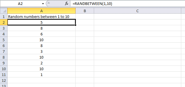
In this example, the RANDBETWEEN function generates random numbers between 2 and 4 with a decimal.
Formula in cell range A2:A11:
Since it actually can't generate numbers with decimals the function generates values between 20 to 40. Divide the output with 10 and the range becomes 2.0 to 4.0.
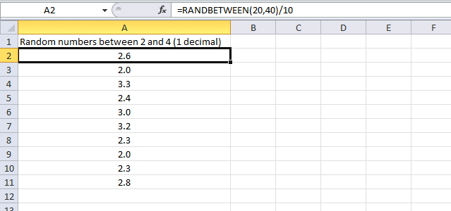
7. Generate negative numbers with two decimals
In this example, the RANDBETWEEN function generates random numbers between -1 and -0.9 with two decimals.
Formula in cell range A2:A11:
The function generates numbers between -100 and -90. The returned number is then divided by 100. The range becomes -1.00 to -0.90.
8. Generate negative numbers with three decimals
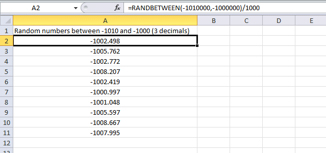
Here, the RANDBETWEEN function generates random negative numbers between -1010.000 and -1000.000
Formula in cell range A2:A11:
The function generates numbers between -1010000 and -1000000. The returned number is then divided by 1000. The range becomes -1010.000 to -1000.000
9. Generate random names
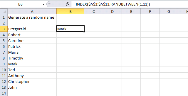
The formula in cell B3 returns random names from cell range A3:A13.
Formula:
Explaining formula in cell B3

I recommend that you use Excel's built-in tool for examining formulas, it is a great feature that allows you to see the calculations steps at a pace you are comfortable with.
Go to tab "Formulas" on the ribbon. Press with mouse on "Evaluate Formula" button to open the "Evaluate Formula" dialog box.
Press with left mouse button on "Evaluate" button to move the calculation to the next step, continue press with left mouse button oning the "Evaluate" button until all steps have been shown. Press with left mouse button on the "Close" to dismiss the dialog box.
Step 1 - Generate random value between 1 and 11
RANDBETWEEN(1,11) returns a number between 1 to 11
Step 2 - Return a value of the cell at the intersection of a particular row and column
The INDEX function allows you to return a value from a given range.
INDEX(array, row_num, [column_num])
INDEX($A$3:$A$13, random_value)
The given range is $A$3:$A$13 and there are 11 cells in that range. Therefore, we need to return a random value between 1 and 11.
RANDBETWEEN(1, 11) returns a number between 1 to 11. The INDEX function then returns a random value from cell range $A$3:$A$13 in cell B3.
You can use the formula in the following post to return unique distinct names: How to create a list of random unique numbers
10. Generate a random list
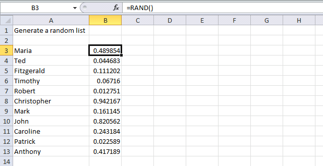
The following steps show you how to randomly shuffle a list. The image above shows names in cell range A3:A13.
- Select cell range B3:B13
- Type =RAND()
- Press and hold CTRL + Enter. This will enter the formula in all cells at once, no need to copy the formula and paste to cells below.
- Select cell range A3:B13
- Press with right mouse button on on the selected cell range.
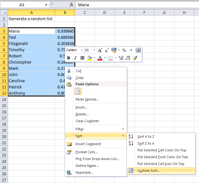
- Press with left mouse button on Sort.
- Press with left mouse button on "Custom Sort..." and a dialog box appears.
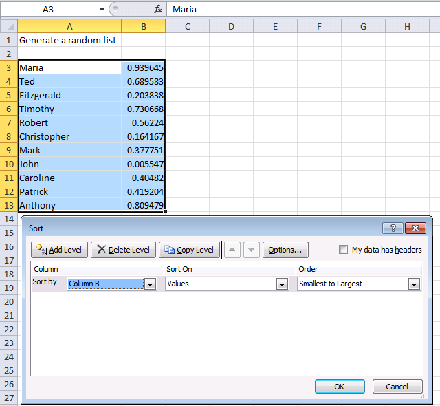
- Sort by: Column B
- Order: Smallest to Largest
- Press with left mouse button on OK button.
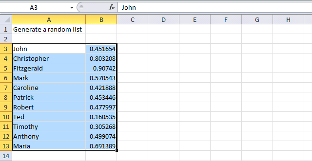
The image above shows the list sorted in a random order.
11. Create random text strings
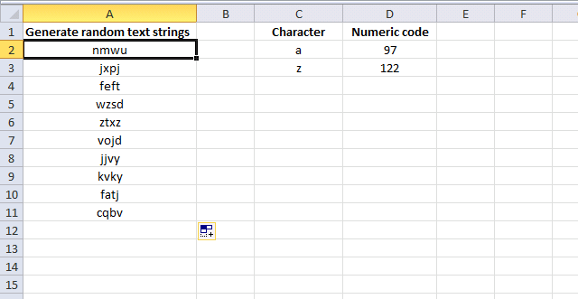
The image above demonstrates a formula in cell range A2:A11 that returns four random characters concatenated into one text string. The characters are lower letters between a and z.
Formula:
Explaining formula in cell A2
Step 1 - Return a random number between 97 and 122
So why return a number between 97 and 122? All characters have a numeric code and the CODE function lets you convert a character to a numeric code.
For example, a is 97 and z is 122. By generating random numbers between 97 and 122 we can create characters from a to z.
RANDBETWEEN(97,122)
Step 2 - Return a character specified by a code number
The CHAR function converts a number to the corresponding character. This is determined by your computer's character set.
CHAR(RANDBETWEEN(97,122))
returns a random character from a to z.
Step 3 - Combine four characters
The ampersand operator & combines different functions to a text string. The are four instances of the formula above, the ampersand concatenates the output from each and returns a text string containing four lower letters.
CHAR(RANDBETWEEN(97,122))& CHAR(RANDBETWEEN(97,122))& CHAR(RANDBETWEEN(97,122))& CHAR(RANDBETWEEN(97,122))
12. Random numbers

This example demonstrates the RAND function returning a number greater than or equal to 0 (zero) and less than 1 each time a worksheet is recalculated.
Formula in cell A1:
Press F9 to recalculate all sheets in all open workbooks, this will also create a new random number in cell A1, see animated image above.
12.1 How can we use this function to return numbers between or equal to 0 and 100?
Formula in cell A3:
ROUNDUP(number, num_digits) rounds a number up, away from zero.

The RANDBETWEEN function is a better choice in this case.
12.2 How to return numbers between or equal to -50 and 50?

Formula in cell A5:
ROUNDUP(number, num_digits) rounds a number up, away from zero.
If you use the RANDBETWEEN function the formula becomes:
13. Random text strings
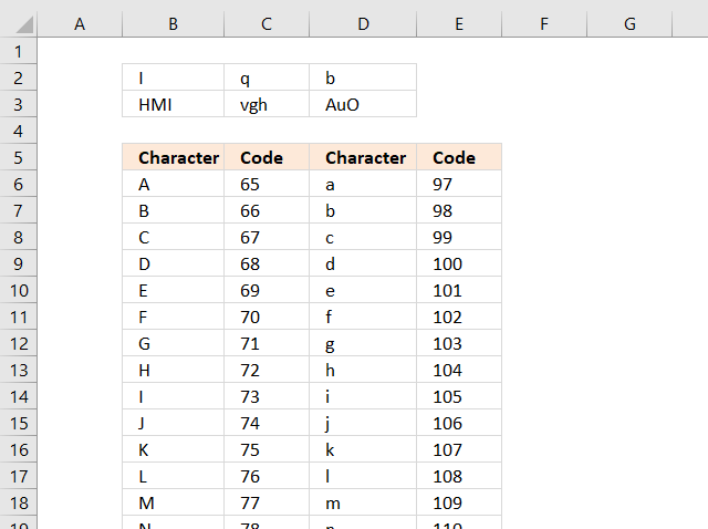
A character in Excel is represented by a number based on the character set, in windows ANSI. A to Z are 65 to 90 and a to z are 97 to 122.
=CHAR(number) returns the character specified by the code number from the character set of your computer.
You can use the CHAR, RAND and ROUNDUP function to return random characters, now let me show you how.
13.1 A random uppercase letter
The following formula returns a single random uppercase letter from A to Z.
Formula in B2:
or use the RANDBETWEEN function which makes the formula smaller and easier to understand.
13.2 A random lowercase letter
The following formula returns a single random lowercase letter from a to z.
Formula in C2:
or a better formula:
13.3 A random lowercase or uppercase letter
This formula returns a random lowercase or uppercase letter.
Formula in D2:
A formula based on the RANDBETWEEN function:
13.4 Three random uppercase letters
This formula concatenates three random uppercase letter A to Z.
Formula in B3:
A formula based on the RANDBETWEEN function:
13.5 Three random lowercase letters
This formula concatenates three random lowercase letter a to z.
Formula in C3
A formula based on the RANDBETWEEN function:
13.6 Three random lowercase and uppercase letters
The forllowing formula returns three random letters that may be lowercase or uppercase.
Formula in D3:
A formula based on the RANDBETWEEN function:
Explaining RANDBETWEEN formula in cell D3
Step 1 - Create arandom number between 0 and 1
The RAND function has no arguments, it simply returns a number between 0 and 1.
RAND()
returns 0.377261423327488 (random number)
Step 2 - If random number is smaller than 0.5
The IF function checks if the logical expression RAND()<0.5 is TRUE or FALSE, if TRUE one thing happens in the second argument and if FALSE another thing happens in the third argument.
IF(RAND()<0.5, CHAR(RANDBETWEEN(65, 90)), CHAR(RANDBETWEEN(97, 122)))
becomes
IF(0.377261423327488<0.5 , CHAR(RANDBETWEEN(65, 90)), CHAR(RANDBETWEEN(97, 122)))
becomes
IF(TRUE , CHAR(RANDBETWEEN(65, 90)), CHAR(RANDBETWEEN(97, 122)))
becomes
CHAR(RANDBETWEEN(65, 90))
and returns a random uppercase letter.
Step 3 - Concatenate characters
The ampersand character concatenates the upper and lower case letter
IF(RAND()<0.5, CHAR(RANDBETWEEN(65, 90)), CHAR(RANDBETWEEN(97, 122)))&IF(RAND()<0.5, CHAR(RANDBETWEEN(65, 90)), CHAR(RANDBETWEEN(97, 122)))&IF(RAND()<0.5, CHAR(RANDBETWEEN(65, 90)), CHAR(RANDBETWEEN(97, 122)))
may become "X"&"h"&"A"
14. Random dates

Excel uses numbers as dates, called the 1900-system. The earliest date you can use is 1900-01-01 and it is represented by number 1. 2012-01-01 is 40909 and is also 40909 days later from the date 1900-01-01.
Now we know how dates in Excel work, let's say you want to create a random number between 2012-01-01 and 2012-12-31. 2012-01-01 is 40909 and 2012-12-31 is 41274. 41274 - 40909 = 365 days.
Now it is time to construct the formula.
Formula in cell A7:
A formula based on the RANDBETWEEN function:
15. Random time values

15.1 Random hours, minutes and seconds
Formula in cell B3:
Cell B3 is formatted as time.
15.2 Random hours
Formula in cell B4:
A formula based on the RANDBETWEEN function:
15.3 Random minutes
Formula in cell B5:
A formula based on the RANDBETWEEN function:
15.4 Random hours and minutes
Formula in cell B6:
A formula based on the RANDBETWEEN function:
15.5 Random minutes and seconds
Formula in cell B7:
16. Assign records unique random text strings

This article demonstrates a formula that distributes given text strings randomly across records in any given day meaning they may be repeated the next day.
The image above shows dates in column B, names in column C and a formula in column D that randomly extracts cell values from column G.
It will make sure that there are no duplicate text strings in any given day.
Vijay asks:
I've 30 objects and 10 people, and I need to assign each person randomly (unique) selected objects as a daily activity. Would you please suggest to me how I can do it using Excel formulae?
The objects are unique within that day. It means that a person can get the same object the next day if unlucky. If this is not what you are looking for, let me know.
The array formula in cell D3:D32 returns a random unique value every time you press F9. The objects are in column F. The table does not need to be sorted by date.
Array formula in cell D3:
How to enter an array formula
- Select cell D3
- Copy above array formula.
- Paste to cell C3.
- Press and hold CTRL + SHIFT simultaneously.
- Press ENTER once.
- Release all keys.
The array formula begins and ends with curly brackets, like this: {=array_formula}. These characters appears automatically and indicate to the user that this is an array formula. Don't enter them yourself.
Excel 365 subscribers have now access to dynamic arrays meaning they don't need to enter the formula as an array formula. Simply press Enter.
This formula returns a single value per cell and will not automatically spill values to cells below.
Explaining array formula in cell D3

(The formula above is not the formula used in this article)
I recommend that you use the "Evaluate Formula" tool located on the ribbon tab "Formulas" to examine any cell formula. This way you can see the all the calculation steps made and also more easily troubleshoot the formula.
- Select cell D3.
- Go to tab "Formulas" on the ribbon.
- Press with left mouse button on the "Evaluate Formula" button and a dialog box appears, see image above.
- Press with mouse on "Evaluate" button located on the dialog box to move to the next calculation step.
- Continue with step 3 until you have seen all calculation steps or press with left mouse button on the "Close" button to dismiss the dialog box.
Step 1 - Identify unique text strings on a given day
The COUNTIFS function counts how many rows meet given criteria. In this case the COUNTIF function returns an array of values, each value in the array corresponds to the position in the unique text string list which is located in $G$3:$G$32.
COUNTIFS(criteria_range1, criteria1, [criteria_range2, criteria2]…)
COUNTIFS($D$2:D2,$G$3:$G$32,$B$2:B2,B3)=0
becomes
{0; 0; 0; 0; 0; 0; 0; 0; 0; 0; 0; 0; 0; 0; 0; 0; 0; 0; 0; 0; 0; 0; 0; 0; 0; 0; 0; 0; 0; 0}=0
and returns
{TRUE; TRUE; TRUE; TRUE; TRUE; TRUE; TRUE; TRUE; TRUE; TRUE; TRUE; TRUE; TRUE; TRUE; TRUE; TRUE; TRUE; TRUE; TRUE; TRUE; TRUE; TRUE; TRUE; TRUE; TRUE; TRUE; TRUE; TRUE; TRUE; TRUE}
This means that all text strings can be randomly selected. If there had been previous object on the same day they would have been ruled out meaning their position in the array would be 1 or higher.
Step 2 - Calculate row numbers
The ROW function calculates the row number from each cell in cell range $G$3:$G$32 and returns an array of row numbers.
MATCH(ROW($G$3:$G$32),ROW($G$3:$G$32))
becomes
MATCH({3; 4; 5; 6; 7; 8; 9; 10; 11; 12; 13; 14; 15; 16; 17; 18; 19; 20; 21; 22; 23; 24; 25; 26; 27; 28; 29; 30; 31; 32},{3; 4; 5; 6; 7; 8; 9; 10; 11; 12; 13; 14; 15; 16; 17; 18; 19; 20; 21; 22; 23; 24; 25; 26; 27; 28; 29; 30; 31; 32})
The MATCH function calculates the relative position of each value in the array against the same array. This step makes sure that the array starts with 1 and increments with 1 up to the total number of values in cell range $G$3:$G$32.
MATCH({3; 4; 5; 6; 7; 8; 9; 10; 11; 12; 13; 14; 15; 16; 17; 18; 19; 20; 21; 22; 23; 24; 25; 26; 27; 28; 29; 30; 31; 32},{3; 4; 5; 6; 7; 8; 9; 10; 11; 12; 13; 14; 15; 16; 17; 18; 19; 20; 21; 22; 23; 24; 25; 26; 27; 28; 29; 30; 31; 32})
returns
{1; 2; 3; 4; 5; 6; 7; 8; 9; 10; 11; 12; 13; 14; 15; 16; 17; 18; 19; 20; 21; 22; 23; 24; 25; 26; 27; 28; 29; 30}
Now we need to multiply the arrays to get the corresponding row number. If the first array contains a zero the result will also be a 0 (zero) for that particular value in the array.
(COUNTIFS($D$2:D2,$G$3:$G$32,$B$2:B2,B3)=0)*MATCH(ROW($G$3:$G$32),ROW($G$3:$G$32))
becomes
{TRUE; TRUE; TRUE; TRUE; TRUE; TRUE; TRUE; TRUE; TRUE; TRUE; TRUE; TRUE; TRUE; TRUE; TRUE; TRUE; TRUE; TRUE; TRUE; TRUE; TRUE; TRUE; TRUE; TRUE; TRUE; TRUE; TRUE; TRUE; TRUE; TRUE}*{1; 2; 3; 4; 5; 6; 7; 8; 9; 10; 11; 12; 13; 14; 15; 16; 17; 18; 19; 20; 21; 22; 23; 24; 25; 26; 27; 28; 29; 30}
and returns
{1; 2; 3; 4; 5; 6; 7; 8; 9; 10; 11; 12; 13; 14; 15; 16; 17; 18; 19; 20; 21; 22; 23; 24; 25; 26; 27; 28; 29; 30}
This array tells us that the formula in cell D3 can pick any of the text strings in column G which makes sense. None of the values have been displayed in cells above cell D3 for that particular date.
Step 3 - Return a random number
In this step, the COUNTIF function counts how many times the corresponding date for cell D3 has occurred in previous cells above.
There are 30 cells in column G that contains text strings, we can't return a random value from column G if we don't keep track of how many values we have displayed in cells above for that particular date.
The first argument in the COUNTIF function contains a cell reference that expands when you copy the cell and paste to cells below as far as needed.
RANDBETWEEN(1,31-COUNTIF($B$2:B3,B3))
becomes
RANDBETWEEN(1, 31-1)
becomes
RANDBETWEEN(1, 30)
The RANDBETWEEN function returns a random value between the numbers you specify.
RANDBETWEEN(1, 30)
returns a random value between 1 and 30.
Step 4 - Return the k-th largest number
The LARGE function returns the k-th largest number from an array or cell range.
LARGE(array, k)
LARGE((COUNTIFS($D$2:D2,$G$3:$G$32,$B$2:B2,B3)=0)*MATCH(ROW($G$3:$G$32),ROW($G$3:$G$32)),RANDBETWEEN(1,31-COUNTIF($B$2:B3,B3)))
becomes
LARGE({1; 2; 3; 4; 5; 6; 7; 8; 9; 10; 11; 12; 13; 14; 15; 16; 17; 18; 19; 20; 21; 22; 23; 24; 25; 26; 27; 28; 29; 30}, RANDBETWEEN(1, 30))
and returns a random row number between 1 and 30.
Step 5 - Return a value
The INDEX function returns a value from cell range $G$3:$G$32 based on the random row number we calculated in the previous step.
INDEX($G$3:$G$32,LARGE((COUNTIFS($D$2:D2,$G$3:$G$32,$B$2:B2,B3)=0)*MATCH(ROW($G$3:$G$32),ROW($G$3:$G$32)),RANDBETWEEN(1,31-COUNTIF($B$2:B3,B3))))
becomes
=INDEX($G$3:$G$32, random_row_number)
becomes
INDEX({"A"; "B"; "C"; "D"; "E"; "F"; "G"; "H"; "I"; "J"; "K"; "L"; "M"; "N"; "O"; "P"; "Q"; "R"; "S"; "T"; "U"; "V"; "X"; "Y"; "Z"; "AA"; "BB"; "CC"; "DD"; "EE"}, random_row_number)
and returns a random text string.
17. Function not working
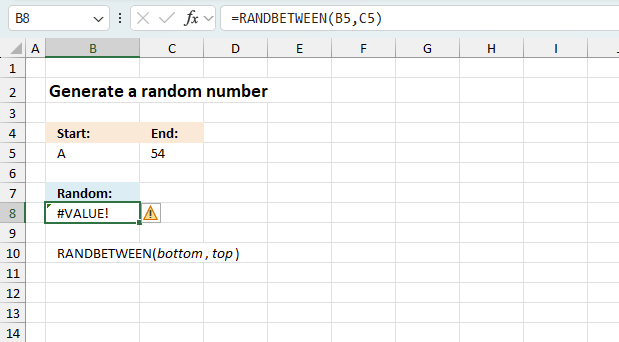
The RANDBETWEEN function returns
- #VALUE! error if you use a non-numeric input value.
- #NAME? error if you misspell the function name.
- propagates errors, meaning that if the input contains an error (e.g., #VALUE!, #REF!), the function will return the same error.
17.1 Troubleshooting the error value
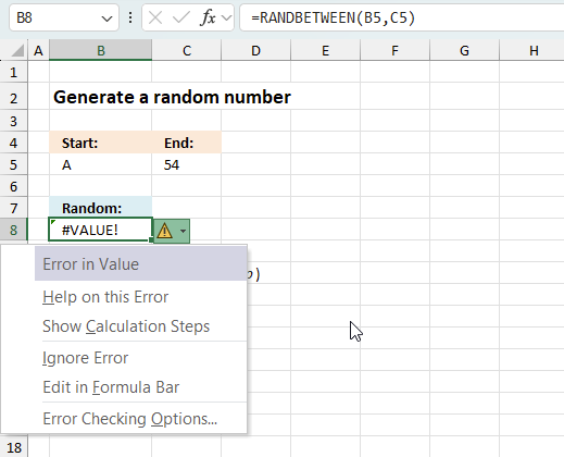
When you encounter an error value in a cell a warning symbol appears, displayed in the image above. Press with mouse on it to see a pop-up menu that lets you get more information about the error.
- The first line describes the error if you press with left mouse button on it.
- The second line opens a pane that explains the error in greater detail.
- The third line takes you to the "Evaluate Formula" tool, a dialog box appears allowing you to examine the formula in greater detail.
- This line lets you ignore the error value meaning the warning icon disappears, however, the error is still in the cell.
- The fifth line lets you edit the formula in the Formula bar.
- The sixth line opens the Excel settings so you can adjust the Error Checking Options.
Here are a few of the most common Excel errors you may encounter.
#NULL error - This error occurs most often if you by mistake use a space character in a formula where it shouldn't be. Excel interprets a space character as an intersection operator. If the ranges don't intersect an #NULL error is returned. The #NULL! error occurs when a formula attempts to calculate the intersection of two ranges that do not actually intersect. This can happen when the wrong range operator is used in the formula, or when the intersection operator (represented by a space character) is used between two ranges that do not overlap. To fix this error double check that the ranges referenced in the formula that use the intersection operator actually have cells in common.
#SPILL error - The #SPILL! error occurs only in version Excel 365 and is caused by a dynamic array being to large, meaning there are cells below and/or to the right that are not empty. This prevents the dynamic array formula expanding into new empty cells.
#DIV/0 error - This error happens if you try to divide a number by 0 (zero) or a value that equates to zero which is not possible mathematically.
#VALUE error - The #VALUE error occurs when a formula has a value that is of the wrong data type. Such as text where a number is expected or when dates are evaluated as text.
#REF error - The #REF error happens when a cell reference is invalid. This can happen if a cell is deleted that is referenced by a formula.
#NAME error - The #NAME error happens if you misspelled a function or a named range.
#NUM error - The #NUM error shows up when you try to use invalid numeric values in formulas, like square root of a negative number.
#N/A error - The #N/A error happens when a value is not available for a formula or found in a given cell range, for example in the VLOOKUP or MATCH functions.
#GETTING_DATA error - The #GETTING_DATA error shows while external sources are loading, this can indicate a delay in fetching the data or that the external source is unavailable right now.
17.2 The formula returns an unexpected value
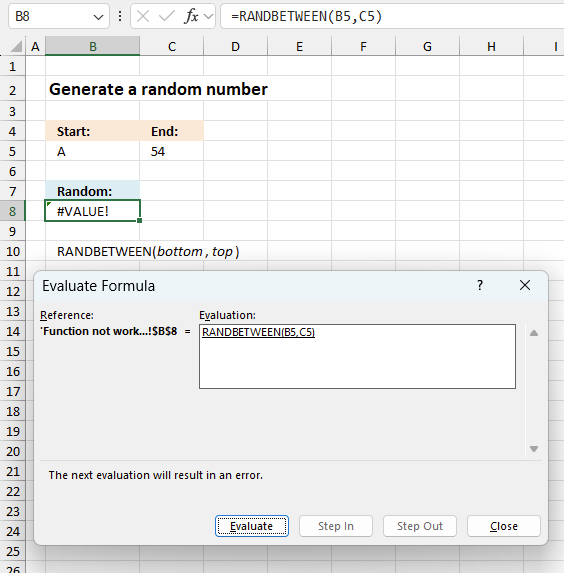
To understand why a formula returns an unexpected value we need to examine the calculations steps in detail. Luckily, Excel has a tool that is really handy in these situations. Here is how to troubleshoot a formula:
- Select the cell containing the formula you want to examine in detail.
- Go to tab “Formulas” on the ribbon.
- Press with left mouse button on "Evaluate Formula" button. A dialog box appears.
The formula appears in a white field inside the dialog box. Underlined expressions are calculations being processed in the next step. The italicized expression is the most recent result. The buttons at the bottom of the dialog box allows you to evaluate the formula in smaller calculations which you control. - Press with left mouse button on the "Evaluate" button located at the bottom of the dialog box to process the underlined expression.
- Repeat pressing the "Evaluate" button until you have seen all calculations step by step. This allows you to examine the formula in greater detail and hopefully find the culprit.
- Press "Close" button to dismiss the dialog box.
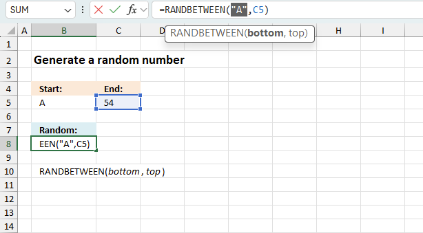
There is also another way to debug formulas using the function key F9. F9 is especially useful if you have a feeling that a specific part of the formula is the issue, this makes it faster than the "Evaluate Formula" tool since you don't need to go through all calculations to find the issue.
- Enter Edit mode: Double-press with left mouse button on the cell or press F2 to enter Edit mode for the formula.
- Select part of the formula: Highlight the specific part of the formula you want to evaluate. You can select and evaluate any part of the formula that could work as a standalone formula.
- Press F9: This will calculate and display the result of just that selected portion.
- Evaluate step-by-step: You can select and evaluate different parts of the formula to see intermediate results.
- Check for errors: This allows you to pinpoint which part of a complex formula may be causing an error.
The image above shows cell reference B5 converted to hard-coded value using the F9 key. The RANDBETWEEN function requires numerical values which is not the case in this example. We have found what is wrong with the formula.
Tips!
- View actual values: Selecting a cell reference and pressing F9 will show the actual values in those cells.
- Exit safely: Press Esc to exit Edit mode without changing the formula. Don't press Enter, as that would replace the formula part with the calculated value.
- Full recalculation: Pressing F9 outside of Edit mode will recalculate all formulas in the workbook.
Remember to be careful not to accidentally overwrite parts of your formula when using F9. Always exit with Esc rather than Enter to preserve the original formula. However, if you make a mistake overwriting the formula it is not the end of the world. You can “undo” the action by pressing keyboard shortcut keys CTRL + z or pressing the “Undo” button
17.3 Other errors
Floating-point arithmetic may give inaccurate results in Excel - Article
Floating-point errors are usually very small, often beyond the 15th decimal place, and in most cases don't affect calculations significantly.
Recommended links
Get the Excel file
Assign-each-person-with-randomly-unique-selected-objects-as-a-daily-activity.xlsx
'RANDBETWEEN' function examples
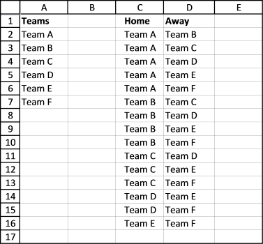
This article demonstrates macros that create different types of round-robin tournaments. Table of contents Basic schedule - each team plays […]
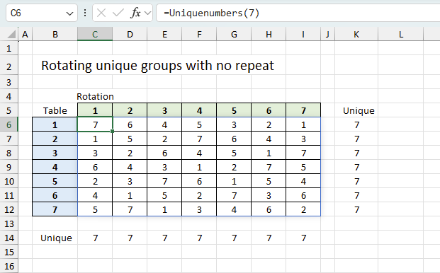
This article demonstrates ways to create unique groups with no repeat. The first example shows a formula that returns random […]
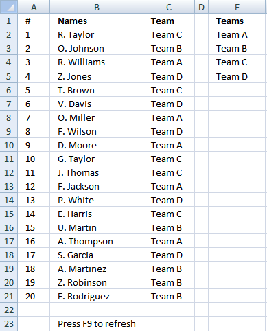
Table of Contents Team Generator Dynamic team generator How to build a Team Generator - different number of people per […]
Functions in 'Math and trigonometry' category
The RANDBETWEEN function function is one of 62 functions in the 'Math and trigonometry' category.
Excel function categories
Excel categories
13 Responses to “How to use the RANDBETWEEN function”
Leave a Reply
How to comment
How to add a formula to your comment
<code>Insert your formula here.</code>
Convert less than and larger than signs
Use html character entities instead of less than and larger than signs.
< becomes < and > becomes >
How to add VBA code to your comment
[vb 1="vbnet" language=","]
Put your VBA code here.
[/vb]
How to add a picture to your comment:
Upload picture to postimage.org or imgur
Paste image link to your comment.
Hi Oscar,
I am trying to do design a random selector similar to this one, the only difference being that the formula I am using selects a random value from a table array using Vlookup.
So far I have a formula of
=VLOOKUP(RANDBETWEEN(1,COUNT($C:$C)),$C$1:$D$10,2,FALSE)
This is cells A1 - A10, there is a numerical place value (and assists with the max value for the randbetween part) in column C, and in column D are the matches. This makes it easy for me to expand/reduce the range quickly and works reasonably well. However, how can I add a condition to make it return a unique value instead of just any, (so that all ten values are alloted) whilst keeping the ease of expansion as the number of matches and returns may differ considerably, but is always at least a 1:1 ratio.
Thanks,
Chris
Chris G,
Array formula in cell B2:
Get the Excel *.xlsx file
Random-unique-values.xlsx
How do you create a random number between -38 and +34 ?
My test sometimes produces numbers outside the low and high.
John
Does this produce numbers outside -38 and 34?
=RANDBETWEEN(-38,34)
Oscar, Thank you for your response.
Yes, the RANDBETWEEN does work with whole numbers.
I misstated the problem. I meant to state: random number between -38.5% and 34.1%. It is the RAND()function that creates numbers outside the High and Low percentages.
Sorry for the confusion.
John
I understand, try this:
=RANDBETWEEN(-385,341)/10
or this
=RANDBETWEEN(-340,340)/1000 and format the cells %.
10-4...worked fine. I used the 1000 divisor in order to create a true percentage result which is then used as a multiplier.
It sure looks simple when you see the answer...guess I just had a V8 moment.
(I still don't know why my RAND() function did not work properly, but am not willing to spend any more time trying to figure it out.)
Thanks again for your help. Keep up the good work.
JB
John,
thank you. I had to google both 10-4 and V8. :-)
How to create a random number and text
Example :
If select cell A1, then result below
KSPC00009000-KSPC00009999
If select cell B1, then result below
KSPR00009000-KSPR00009999
Atha,
Cell A1:
="KSPC0000"&RANDBETWEEN(9000,9999)
Cell B1:
="KSPR0000"&RANDBETWEEN(9000,9999)
Mr Oscar, thanks for your help, its work for me.
Mr Oscar,
How to Generate a New Number & Text to case below (VBA) :
textbox1 : save the result in Cell A2
commandbutton1 : Generate new random ie KSPC00009000-KSPC00009999
Generate a new number and not duplicate with range A2:A100
If there's a duplicate, then generate a new number again, until there's a unique value, save it and proceed to the next until it is finished.
I've tried this code but not running in case number & text
Private Sub cmdGenerate_Click()
    Dim Low As Long
    Dim High As Long
    Dim r As Long

    Low = 9000
    High = 9999
getNum:
    r = "KSPC0000" & Int((High - Low + 1) * Rnd() + Low)
    If IsNumeric(Application.Match(r, Worksheets("Sheet1").Range("A:A"), False)) Then GoTo getNum
    Worksheets("Sheet1").Cells(Rows.Count, "A").End(xlUp)(2).Value = r
    Me.Textbox1.Value = r

End Sub
Thanks
Dear Oscar,
Thank you for your efforts. I was looking for the same and came to your post and excel file. I have extended the list as I have a longer list. I'm having an issue that only first value is duplicating whereas the rest it is fine. After keep pressing F9 again and again; the duplicate disappear at time but later again it disappear.
(Screenshot attached)
https://s4.postimg.org/s7is63uu5/Screenshot_2017-08-01_15.52.02.png
can you please help me.