Search for a text string in a data set and return multiple records
This article explains different techniques that filter rows/records that contain a given text string in any of the cell values in a record. To filter records based on a condition read this: VLOOKUP - Extract multiple records based on a condition, that article also demonstrates how to filter records using the new FILTER function only available in Excel 365.
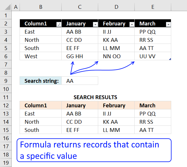
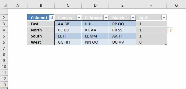
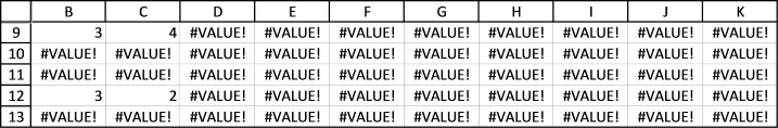
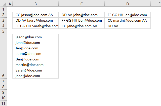
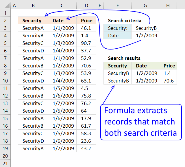
Example, the image above shows the data in cell range B3:E6, the condition is in cell C9. The formula extracts records from B3:E6 if at least one cell contains the string.
Row 3 is extracted above because string AA is found in cell C3. Row 4 and 5 are also extracted because string AA is found in cell D4 and E5 respectively. Row 6 is not extracted, there is no cell containing the search string.
Read section 1.1 for a detailed explanation of how this formula works. I have built a formula that matches two criteria and return multiple records.
What is on this page?
- Search for a text string in a data set and return multiple records [Array formula]
- Search for a text string in a data set and return multiple records [Excel 365]
- Search for a text string in a data set and return multiple records [Excel defined Table]
- Search for a text string in a data set and return multiple records [Advanced Filter]
- Get Excel file
- Exact word in string
- Partial match based on two conditions in any column- both must match
- Partial match with two conditions - one condition for each column
- Partial match with two conditions - one for each column - Excel 365
- Partial match with three conditions - one for each column
- Lookup with multiple criteria and display multiple search results (VBA)
- Search each column for a string each and return multiple records - OR logic
- How to extract rows containing digits
- How to extract email addresses from an Excel sheet
- Filter words containing a given string in a cell range - Excel 365 LAMBDA function
- Filter words containing a given string in a cell range - User Defined Function
- Filter unique distinct words from a cell range - Excel 365
- Filter unique distinct words from a cell range - UDF
1. Search for a text string in a data set and return multiple records [Array formula]

This example demonstrates a formula that extracts records if any cell on the same row contains a specific value specified in cell C9.
This means also that the formula returns the same record multiple times if multiple cells contain the search value.
Array formula in B13:
To enter an array formula, type the formula in cell B13 then press and hold CTRL + SHIFT simultaneously, now press Enter once. Release all keys.
The formula bar now shows the formula with a beginning and ending curly bracket telling you that you entered the formula successfully. Don't enter the curly brackets yourself.
Copy cell B13 and paste to cell range B13:E16. Replace FIND function with SEARCH function if you don't want the formula to perform a case-sensitive search.
Search for a text string in a data set and return multiple records (no duplicates)
Array formula in cell B13:
The array formula above returns unique distinct records meaning no duplicate records if more than one cell matches the search string.
1.1 Explaining array formula in cell B13
Step 1 - Identify cells containing the search string
The FIND function returns the starting point of one text string within another text string, it returns a number representing the position of the found string. If not found the function returns the #VALUE! error.
FIND($C$9, $B$3:$E$6)
returns
{#VALUE!, 1, #VALUE!, ... , #VALUE!}
The ISNUMBER function returns TRUE if the value in the array is a number and FALSE if not a number, it returns FALSE even if the value is an error value which is handy in this case.
ISNUMBER(FIND($C$9, $B$3:$E$6)) creates this array displayed in cell B11:E14:
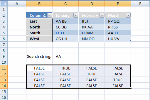
Column B has no cells containing string "AA".
Column C has 1 cell containing string "AA". Cell C3
Column D has 1 cell containing string "AA". Cell D4.
Column E has 1 cell containing string "AA". Cell E5.
Step 2 - Return row number
We need to calculate the row number for each cell in order to replace TRUE in the array with the corresponding row number. To create the array we need we use the MATCH function and the ROW function.
MATCH(ROW(Table1), ROW(Table1)) returns this array displayed in cell range B11:E14:

If string "AA" is found in a cell in the table the corresponding row number is returned.
Step 3 - Replace boolean values with row numbers
The IF function has three arguments, the first one must be a logical expression. If the expression evaluates to TRUE then one thing happens (argument 2) and if FALSE another thing happens (argument 3).
IF(ISNUMBER(FIND($C$9, Table1)), MATCH(ROW(Table1), ROW(Table1)), "")
returns the following array shown in cell range B11:E14:

Step 4 - Sort the row numbers from smallest to largest
To be able to return a new value in a cell each I use the SMALL function to filter column numbers from smallest to largest.
The ROWS function keeps track of the numbers based on an expanding cell reference. It will expand as the formula is copied to the cells below.
SMALL(IF(ISNUMBER(FIND($C$9, Table1)), MATCH(ROW(Table1), ROW(Table1)), ""), ROWS($A$1:A1))
returns 1.
Step 5 - Return a value at the intersection of a particular row and column
The INDEX function returns a value based on a cell reference and column/row numbers.
INDEX(Table1, SMALL(IF(ISNUMBER(FIND($C$9, Table1)), MATCH(ROW(Table1), ROW(Table1)), ""), ROWS($A$1:A1)), COLUMNS($A$1:A1))
returns "East" in cell B13.
Step 6 - Remove errors
The IFERROR function allows you to display a blank if the formula returns an error.
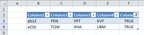
2. Search for a text string in a data set and return multiple records [Excel 365]

The image above demonstrates an Excel 365 formula that extracts records based on a condition. The record is extracted if any cell in a record contains the condition.
Dynamic array formula in cell B13:
This formula works only in Excel 365, it returns an array of values that spills to cells below and to the right automatically. The formula contains the new FILTER function.
2.1 Explaining formula in cell B13
Step 1 - Identify cells containing the given search string
The FIND function returns the position of a specific string in another string, reading left to right. Note, the FIND function is case-sensitive.
FIND(C9, Table1)
returns {#VALUE!, 1, #VALUE!, ... , #VALUE!}.
The FIND function returns a #VALUE! error if no string is found.
Step 2 - Check if value in array is a number
The ISNUMBER function returns a boolean value TRUE or FALSE. TRUE if the value is a number and FALSE for anything else, also an error value.
ISNUMBER(FIND(C9, Table1))
returns {FALSE, TRUE, FALSE, ... , FALSE}.
Step 3 - Convert boolean values to numerical equivalents
The asterisk lets you multiply a value or array, this action converts boolean values to numbers automatically. This step is required because the MMULT function can't work with boolean values.
ISNUMBER(FIND(C9, Table1))*1
becomes
{FALSE, TRUE, FALSE, ... , FALSE} * 1
and returns
{0, 1, 0, 1; 0, 0, 1, 0; 0, 0, 0, 1; 0, 0, 0, 0}.
Step 4 - Create a number sequence
The ROW function calculates the row number of a cell reference.
ROW(ref)
ROW(Table1)
returns {3; 4; 5; 6}.
Step 5 - Change numbers to 1
The power of or exponent character is able to convert each number if number to the power of zero is calculated.
ROW(Table1)^0
becomes
{3; 4; 5; 6}^0
and returns {1; 1; 1; 1}.
Step 6 - Consolidate numbers
The MMULT function calculates the matrix product of two arrays, an array as the same number of rows as array1 and columns as array2.
MMULT(array1, array2)
MMULT(ISNUMBER(FIND(C9, Table1))*1, ROW(Table1)^0)
becomes
MMULT({0, 1, 0, 1; 0, 0, 1, 0; 0, 0, 0, 1; 0, 0, 0, 0}, {1; 1; 1; 1})
and returns {2; 1; 1; 0}.
Step 7 - Filter values based on array
The FILTER function lets you extract values/rows based on a condition or criteria.
FILTER(array, include, [if_empty])
FILTER(Table1, MMULT(ISNUMBER(FIND(C9, Table1))*1, ROW(Table1)^0))
becomes
FILTER(Table1, {2; 1; 1; 0})
and returns the following array in cell B13:
{"East", "AA BB", "II JJ", "PP QQ AA"; "North", "CC DD", "KK AA", "RR SS"; "South", "EE FF", "LL MM", "AA TT"}
3. Search for a text string in a data set and return multiple records - Excel Table
This example demonstrates how to filter records if any of the cells on a row contains a specific string using an Excel Table. You need a formula and a helper column to accomplish this task.
You can't do this using the "Custom Autofilter" built-in to the Excel Table, there is no way to use OR logic between filters across columns, you need a formula to do this. As far as I know.
3.1 Convert dataset to an Excel defined Table
- Select any cell within the dataset.
- Press CTRL + T
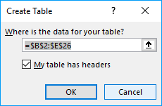
- Press with left mouse button on checkbox if your dataset contains headers for each column.
- Press with left mouse button on OK button.
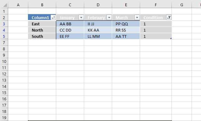
3.2 Add formula to Excel defined Table
- Select cell F3.
- Type formula: =COUNTIF(Table13[@[January]:[March]],"*AA*")
- Press Enter.
Excel fills the remaining cells in the table for you and creates a header name for your new column automatically.
3.3 Explaining formula in cell F3
Step 1 - COUNTIF function
The COUNTIF function calculates the number of cells that is equal to a condition.
COUNTIF(range, criteria)
Step 2 - Populate arguments
COUNTIF(Table13[@[January]:[March]],"*AA*")
range - Table13[@[January]:[March]] is a structured reference to data in columns January to March in table Table13. The at sign @ before the header names indicate that the reference is to values on the same row.
criteria - "*AA*" The asterisk character is a wildcard character that matches 0 (zero) to any number of characters. When we use a leading and trailing asterisk the criteria matches cells that contain "AA".
Step 3 - Evaluate formula
COUNTIF(Table13[@[January]:[March]],"*AA*")
becomes
COUNTIF({"AA BB", "II JJ", "PP QQ"}, "*AA*")
and returns 1 in cell F3. String AA was found once in cell range C3:E3. Note that the formula evaluates only cells on the same row, this is why the formula doesn't return an array of values.
3.4 Filter Excel Table
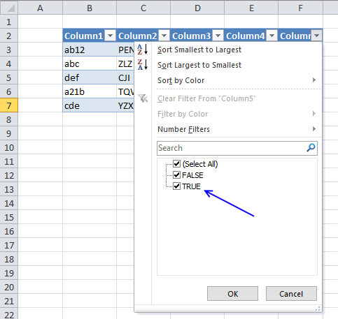
To filter the records containing string AA at least once follow these steps:
- Press with left mouse button on black arrow next to the header name "April".
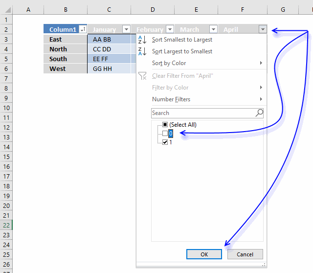
- Press with left mouse button on checkbox next to 0 (zero) to deselect it.
- Press with left mouse button on OK button.
April is not the correct header name, I changed it to Condition.
4. Search for a text string in a data set and return multiple records [Advanced Filter]
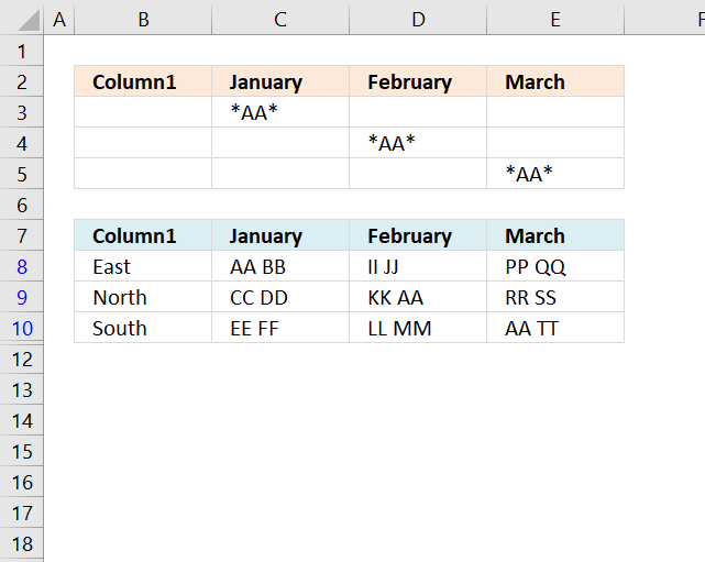
The Advanced Filter is a powerful feature in Excel that allows you to perform OR-logic between columns. The asterisk lets you do a wildcard lookup meaning that a record is filtered if the text string is found somewhere in the cell value.
4.1 Add columns
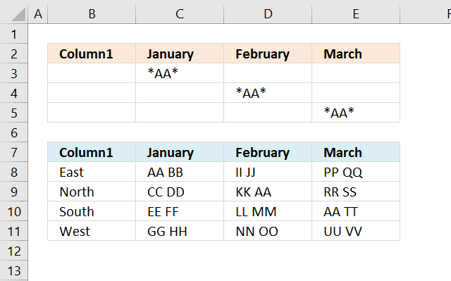
- Copy column headers and paste to cells above or below the dataset. Note, if you place them next to the dataset they may become hidden when the filter is applied.
- Type the search condition and add an asterisk before and after the text string.
- Add another search condition, make sure they are in a row each in order to perform OR-logic.
- Repeat with the remaining criteria.
4.2 Apply filter
- Select the dataset.
- Go to tab "Data" on the ribbon.
- Press with left mouse button on the "Advanced" button.
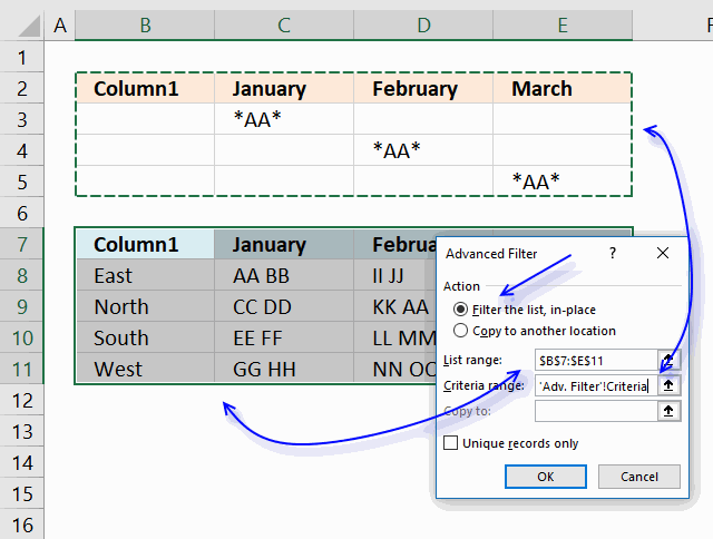
- Press with left mouse button on the radio button "Filter the list, in-place".
- Select Criteria range:"
- Press with left mouse button on "OK button.
To delete the filter applied simply select a cell within the filtered dataset, then go to tab "Data" on the ribbon and press with left mouse button on "Clear" button.
5. Excel file
How do I extract rows that contain a string in a data set or table?
You can use a formula to extract records based on a search value, it also returns multiple records if there are any that match. The advantage of using a formula is that it is dynamic meaning the result changes as soon as a new search value is entered. The downside with the formula is that it may become slow if you have lots of data to work with.
How do I filter rows that contain a string using Advanced Filter?
You also have the option to filter records using an Advanced Filter, it allows you to perform multiple search values using OR-logic across multiple columns. This article explains how to set it up, jeep in mind that it needs a small amount of manual work in order to apply new filters.
How do I filter rows that contain a string using an Excel defined Table?
The Excel defined Table needs the COUNTIF function to accomplish the task which may slow down the calculation considerably if your data set is huge. I recommend using the Advanced Filter if speed is an issue.
6. Exact word in string
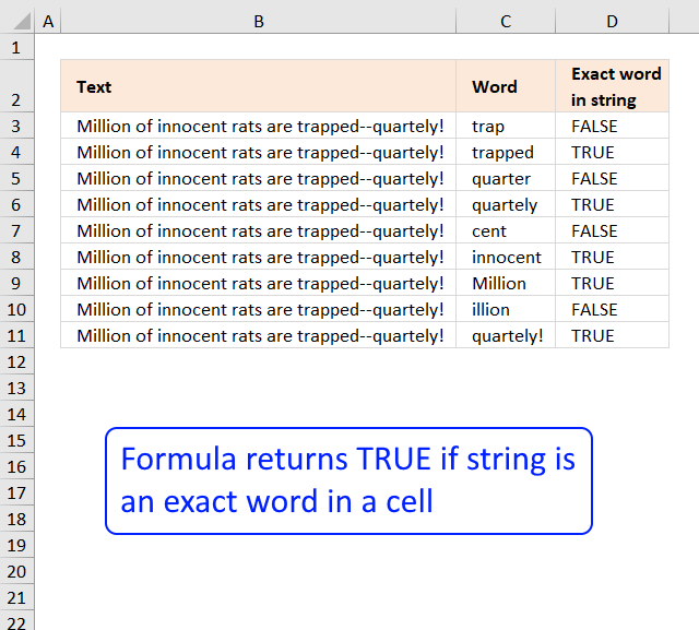
I read an interesting blog post Is A Particular Word Contained In A Text String? on Spreadsheetpage. That inspired me to create an excel formula doing the same thing as the vba function.
In short, from the above blog post
The function, modified the first argument (Text) and replaces all non-alpha characters with a space character. It then adds a leading and trailing space to both arguments. Finally, it uses the Instr function to determine if the modified Word argument is present in the modified Text argument
The ExactWordInString function looks for a complete word -- not text that might be part of a different word.

Edit: Read Rick Rothstein (MVP - Excel) comments at the bottom of this blog post.
Here is the formula I created in C2:
copied down as far as necessary.
Explaining formula in cell C2
Step 1 - Check if string exists in cell
The FIND function returns the position of a string in cell value, if not found an error is returned. The ISNUMBER function returns TRUE for all numerical values and FALSE for all else even error values.
The IF function uses the boolean value to determine if the first argument or second argument is going to be returned.
IF(ISNUMBER(FIND(B2, A2)), formula, FALSE)
becomes IF(TRUE, formula, FALSE)
The IF function now continues the calculation with the first argument formula.
Step 2 - Check if the character before the string is larger than ansi code 122
The CODE function converts a character into ansi equivalent. Character "A" is 65 and "z" is 122.
COUNT((IF(CODE(MID(A2,FIND(B2,A2)-1,1))>122,1,""))
returns 0.
Step 3 - Check if character before the string is less than ansi code 65
The MID function extracts a part of a string based on a start character and the length.
IF(CODE(MID(A2,FIND(B2,A2)-1,1))<65,1,"")
and returns 1.
Step 4 - Check if string is at the very beginning
IF(FIND(B2,A2)-1<1,1,"")
and returns "".
Step 5 - Check if the character after the string is larger than ansi code 122
The LEN function counts characters in a cell.
COUNT((IF(CODE(MID(A2,FIND(B2,A2)+LEN(B2),1))>122,1,""))
and returns 0.
Step 6 - Check if character after the string is less than ansi code 65
The IF function returns a value determined by the logical expression in the first argument. If TRUE then the second argument is returned, FALSE returns the third argument.
IF(CODE(MID(A2,FIND(B2,A2)+LEN(B2),1))<65,1,"")
and returns "".
Step 7 - Check if string is at the very end
IF((FIND(B2,A2)+LEN(B2)+1)>LEN(A2),1,"")
and returns "".
Step 8 - Nested IFs
All these IF functions are nested.
Get Excel *.xlsx file
Exact word in string using excel functions.xlsx
7. Partial match based on two conditions in any column- both must match
Question:
Answer:
Excel 365 dynamic array formula in cell E7:
The Excel 365 formula above is not only smaller but also allows you to easily increase the number of conditions. Simply change cell ref F2:F3 to almost any number of conditions, remember that all search strings must be found on the same row for it to match.
The formula above also lets you also use a data source larger than two columns, this is not the case with the older formula below unless you modify it to your needs.
Advantages of the Excel 365 formula above compared to the older formula below.
- Almost any number of search strings
- Almost any data source range size
- Easy to modify cell references
- No need to enter the formula as an array formula
- Spills values automatically to cells below and to the right as far as needed
Array formula in cell E7:
How to create an array formula
- Select cell D7
- Press with left mouse button on in formula bar
- Copy and paste array formula to formula bar
- Press and hold Ctrl + Shift
- Press Enter
- Release all keys
How to copy an array formula
- Select cell D7
- Copy the cell (Ctrl + c)
- Select cell range D7:D12
- Paste (Ctrl + v)
- Copy cell range D7:D12 (Ctrl + c)
- Select cell range E7:E12
- Paste (Ctrl + v)
Explaining formula in cell D7
Step 1 - Search $B$3:$C$17 for value in cell $F$2
The SEARCH function returns the relative position of the search string, if nothing found then the function returns an #VALUE! error.
SEARCH($F$2,$B$3:$C$17)
and returns {#VALUE!,#VALUE!; ... ,3}
Step 2 - Convert array to boolean values
The ISNUMBER function coonverts errors into TRUE and remaining values into FALSE.
ISNUMBER(SEARCH($F$2,$B$3:$C$17))*1
becomes
{FALSE,FALSE;TRUE, ... ,TRUE}*1
The MMULT function can't work with boolean values, we must multiply with 1 to convert boolean values into numerical equivalents:
The following image shows the array in cell range E3:F17.
Step 3 - Sum values on each row
The MMULT function sums values row-wise.
returns {FALSE;TRUE; FALSE;... ; TRUE}
The array is entered in column G, it is now very clear that MMULT function sums values on each row.
Step 4 - Search string 2
This step demonstrates the same steps 1 to 3, however, the search string is in cell E3
(MMULT(ISNUMBER(SEARCH($E$3,$B$3:$C$17))*1,{1;1})>0)
returns
{TRUE;FALSE; TRUE;... ; TRUE}
Step 5 - Multiply arrays
Both conditions must be met in other words both strings must have been found in a row, see table below.
| Boolean | Boolean | Result |
| FALSE | FALSE | 0 |
| TRUE | FALSE | 0 |
| TRUE | TRUE | 1 |
(MMULT(ISNUMBER(SEARCH($L$2,$B$3:$C$17))*1,{1;1})>0)*(MMULT(ISNUMBER(SEARCH($L$3,$B$3:$C$17))*1,{1;1})>0)
returns {0;0; 0;0; 1;1; 0;0; 1;0; 0;0; 1;0; 1}
Step 6 - Replace TRUE with corresponding row number
IF((MMULT(ISNUMBER(SEARCH($L$2,$B$3:$C$17))*1,{1;1})>0)*(MMULT(ISNUMBER(SEARCH($L$3,$B$3:$C$17))*1,{1;1})>0),MATCH(ROW($B$3:$C$17),ROW($B$3:$C$17)),"")
returns {"";"";"";"";5;6;"";"";9;"";"";"";13;"";15}.
Step 7 - Extract k-th smallest row number
SMALL(IF((MMULT(ISNUMBER(SEARCH($L$2,$B$3:$C$17))*1,{1;1})>0)*(MMULT(ISNUMBER(SEARCH($L$3,$B$3:$C$17))*1,{1;1})>0),MATCH(ROW($B$3:$C$17),ROW($B$3:$C$17)),""),ROWS($A$1:A1))
becomes
SMALL({"";"";"";"";5;6;"";"";9;"";"";"";13;"";15},ROWS($A$1:A1))
The ROWS function returns the number of rows in a cellreference, this cell reference expands when formula is copied to cells below. This makes sure a new row number is extracted and returned in each cell.
SMALL({"";"";"";"";5;6;"";"";9;"";"";"";13;"";15},1)
and returns 5.
Step 8 - Return value
The INDEX function gets a number based on row and column numbers.
INDEX($B$3:$C$17, SMALL(IF((MMULT(ISNUMBER(SEARCH($F$2, $B$3:$C$17))*1, {1;1})>0)*(MMULT(ISNUMBER(SEARCH($F$3, $B$3:$C$17))*1, {1;1})>0), MATCH(ROW($B$3:$C$17), ROW($B$3:$C$17)), ""), ROWS($A$1:A1)), COLUMNS($A$1:A1))
returns "Roddick" in cell E7.
Get Excel *.xlsx file
multiple-criteria-lookup-with-multiple-results-2v4.xlsx
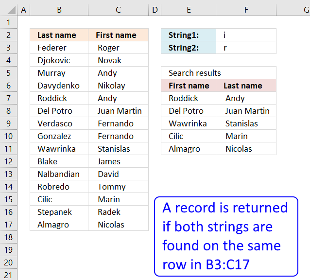
8. Partial match with two conditions - one condition for each column
Question:
How do I search a list containing two columns? I want to search both columns at the same time with two different criteria (one criteria for each column) and then display multiple search results.

Answer

I created two search fields. First and last name in F2 and F3. The search results are presented in columns D and E. See the picture below.
The array formula in cell E8:
1.1 How to create an array formula
- Copy (Ctrl + c) and paste (Ctrl + v) array formula into formula bar.
- Press and hold CTRL + SHIFT keys.
- Press Enter key once.
- Release all keys.
Recommended articles

Array formulas allows you to do advanced calculations not possible with regular formulas.
Copy cell D6 and paste it to cells below and to the right as far as needed.
1.2 Explaining the array formula in cell D6
Step 1 - Find the first partial match
The SEARCH function returns the number of the character at which a specific character or text string is found reading left to right (not case-sensitive)
SEARCH(find_text,within_text, [start_num])
SEARCH($F$2, $C$3:$C$17)
returns {5; #VALUE!; #VALUE!; ... ; #VALUE!}.
Step 2 - Second partial match
SEARCH($F$3, $B$3:$B$17)
returns {#VALUE!; 3; ... ; 7}.
Step 3 - Multiply arrays
The asterisk character lets you multiply the arrays creating AND logic meaning both values in the same position must be a number. This will only match rows where both conditons are met.
(SEARCH($F$2, $C$3:$C$17))*(SEARCH($F$3, $B$3:$B$17))
returns {#VALUE!; #VALUE!; #VALUE!; ... ; #VALUE!}.
Step 4 - Check if the value is a number
The array calculated in the previous step has error values that we must take care of. The ISNUMBER function returns TRUE if a value in the array is a number and FALSE for everything else including error values.
ISNUMBER((SEARCH($F$2, $C$3:$C$17))*(SEARCH($F$3, $B$3:$B$17)))
returns {FALSE; FALSE; FALSE; ... ; FALSE}.
Step 5 - Replace boolean values with corresponding row numbers
The IF function returns one value if the logical test is TRUE and another value if the logical test is FALSE.
IF(logical_test, [value_if_true], [value_if_false])
IF(ISNUMBER((SEARCH($F$2, $C$3:$C$17))*(SEARCH($F$3, $B$3:$B$17))), MATCH(ROW($B$3:$B$17), ROW($B$3:$B$17)), "")
The ROW function lets you create numbers representing the rows based on a cell range.
The MATCH function finds the relative position of a given string in an array or cell range. This will create an array from 1 to n where n is the number of rows in cell range $B$3:$B$17.
returns {""; ""; ""; ""; ""; ""; 7; 8; ""; ""; ""; ""; ""; ""; ""}.
Step 6 - Extract k-th smallest row number
The SMALL function returns the k-th smallest value from a group of numbers.
SMALL(array, k)
SMALL(IF(ISNUMBER((SEARCH($F$2, $C$3:$C$17))*(SEARCH($F$3, $B$3:$B$17))), MATCH(ROW($B$3:$B$17), ROW($B$3:$B$17)), ""), ROWS($A$1:A1))
returns 7.
Step 7 - Get value from B3:C17 based on row and column number
The INDEX function returns a value from a cell range, you specify which value based on a row and column number.
INDEX($B$3:$C$17, SMALL(IF(ISNUMBER((SEARCH($F$2, $C$3:$C$17))*(SEARCH($F$3, $B$3:$B$17))), MATCH(ROW($B$3:$B$17), ROW($B$3:$B$17)), ""), ROWS($A$1:A1)), COLUMNS($A$1:A1))
returns ""Verdasco" in cell E8.
9. Partial match with two conditions - one for each column - Excel 365
Question:
How do I search a list containing two columns? I want to search both columns at the same time with two different criteria (one criteria for each column) and then display multiple search results.
Answer:

The image above shows a dynamic array formula that is much shorter than the formula in section 1 for previous Excel versions.
Excel 365 dynamic array formula in cell E8:
Explaining formula in cell E8
Step 1 - Partial match first condition
The SEARCH function returns the number of the character at which a specific character or text string is found reading left to right (not case-sensitive)
SEARCH(find_text,within_text, [start_num])
SEARCH($F$2, $C$3:$C$17)
{5; #VALUE!; #VALUE!; ... ; #VALUE!}.
Step 2 - Partial match second condition
SEARCH($F$3, $B$3:$B$17)
returns {#VALUE!; 3; ... ; 7}.
Step 3 - AND logic
The asterisk character lets you multiply the arrays creating AND logic meaning both values in the same position must be a number. This will only match rows where both conditons are met.
SEARCH($F$2, $C$3:$C$17)*SEARCH($F$3, $B$3:$B$17)
returns {#VALUE!; #VALUE!; #VALUE!;... ; #VALUE!}.
Step 4 - Check if number
The array calculated in the previous step has error values that we must take care of. The ISNUMBER function returns TRUE if a value in the array is a number and FALSE for everything else including error values.
ISNUMBER((SEARCH($F$2, $C$3:$C$17))*(SEARCH($F$3, $B$3:$B$17)))
returns {FALSE; FALSE; FALSE; ... ; FALSE}.
Step 5 - Extract records
The FILTER function lets you extract values/rows based on a condition or criteria. It is in the Lookup and reference category and is only available to Excel 365 subscribers.
FILTER(array, include, [if_empty])
FILTER($B$3:$C$17, ISNUMBER(SEARCH($F$2, $C$3:$C$17)*SEARCH($F$3, $B$3:$B$17)))
returns {"Verdasco", " Fernando "; "Gonzalez", " Fernando "}.
10. Partial match with three conditions - one for each column
Can expand this equation set into more than two colums of data, say if I had a first, middle and last name column could I only display the values in which all three cases are true?This blog article answers a question in this article: Lookup with multiple criteria and display multiple search results using excel formula
Excel 365 dynamic array formula in cell F8:
The formula above spills values to cells below and to the right as far as needed. It is also highly customizable, you can easily add or remove conditions, however, the number of conditions must match the number of columns based on the original data (B3:D17) source.
If one of the conditions is blank then the condition is not evaluated at all, this is true for both the older formula below and the newer above.
Array formula in F8:
To enter an array formula, type the formula in a cell then press and hold CTRL + SHIFT simultaneously, now press Enter once. Release all keys.
The formula bar now shows the formula with a beginning and ending curly bracket telling you that you entered the formula successfully. Don't enter the curly brackets yourself.
Explaining formula in cell F8
Step 1 - Search for criteria
The SEARCH function allows you to find a string in a cell and it's position. It also allows you to search for multiple strings in multiple cells if you arrange values in a way that works. That is why I use the TRANSPOSE function to transpose the values.
SEARCH(TRANSPOSE($G$2:$G$4), $B$3:$D$17)
returns {#VALUE!, #VALUE!, 3;... , 5}.
Step 2 - Convert numbers to true
The ISNUMBER function returns TRUE if value is a number and FALSE for everything else even errors which is very handy in this case, the search function returns #VALUE! error if a string is not found in a particular cell.
--(ISNUMBER(SEARCH(TRANSPOSE($G$2:$G$4), $B$3:$D$17)))
returns
--({FALSE, FALSE, TRUE;... , TRUE})
The MMULT function can't work with boolean values so we need to convert them into their numerical equivalents. TRUE - 1 annd FALSE - 0 (zero).
returns
{0, 0, 1; ... , 1}
Step 3 - Sum values row-wise
MMULT(--(ISNUMBER(SEARCH(TRANSPOSE($G$2:$G$4), $B$3:$D$17))), {1;1;1})
returns {1; 1; 1; 3; 0; 0; 3; 2; 1; 1; 1; 2; 0; 1; 2}
Step 4 - Convert non-numerical values to corresponding row numbers
The following IF function returns the row number if number is 3, there are three strings that must match. FALSE returns "" (nothing).
IF(MMULT(--(ISNUMBER(SEARCH(TRANSPOSE($G$2:$G$4), $B$3:$D$17))), {1; 1; 1})=3, MATCH(ROW($B$3:$D$17), ROW($B$3:$D$17)), "")
returns {"";"";"";4;"";"";7;"";"";"";"";"";"";"";""}.
Step 5 - Extract k-th smallest value in array
The SMALL function makes sure that a new value is returned in each row.
SMALL(IF(MMULT(--(ISNUMBER(SEARCH(TRANSPOSE($G$2:$G$4), $B$3:$D$17))), {1; 1; 1})=3, MATCH(ROW($B$3:$D$17), ROW($B$3:$D$17)), ""), ROWS($A$1:A1))
The ROWS function returns a new number because the cell reference expands as the formula is copied to cells below.
returns 4.
Step 6 - Return value
The INDEX function returns a value based on a row and column number.
INDEX($B$3:$D$17, SMALL(IF(MMULT(--(ISNUMBER(SEARCH(TRANSPOSE($G$2:$G$4), $B$3:$D$17))), {1; 1; 1})=3, MATCH(ROW($B$3:$D$17), ROW($B$3:$D$17)), ""), ROWS($A$1:A1)), COLUMNS($A$1:A1))
returns "Davydenko" in cell F8.
Get Excel *.xlsx file
multiple criteria lookup with multiple resultsv2.xlsx
11. Lookup with multiple criteria and display multiple search results (VBA)

Where to copy vba code
- Copy vba code below
- Press Alt + F11
- Insert a new module
- Paste code into code window
- Return to Excel
Array Formula in cell E9:
=Searchtbl(F2:F4;A2:C16)
How to create array formula
- Select cell range E9:G11
- Type above array formula
- Press and hold Ctrl + Shift
- Press Enter once
- Release alla keys
Function Searchtbl(SrchRng As Variant, tbl As Variant) As Variant
'SrchRng must have equal number of cells as headers in table
Dim i, r, c As Single
Dim tempArray() As Variant
ReDim tempArray(tbl.Columns.Count - 1, 0)

tbl = tbl.Value
SrchRng = SrchRng.Value

For r = LBound(tbl, 1) To UBound(tbl, 1)
    i = 0
    For c = LBound(SrchRng) To UBound(SrchRng)
        If InStr(UCase(tbl(r, c)), UCase(SrchRng(c, 1))) = 0 Then
            i = 0
            Exit For
        Else
            i = i + 1
        End If
    Next c

    If i = UBound(tbl, 2) Then
        For c = LBound(tempArray, 1) To UBound(tempArray, 1)
            tempArray(c, UBound(tempArray, 2)) = tbl(r, c + 1)
        Next c
        ReDim Preserve tempArray(UBound(tempArray, 1), UBound(tempArray, 2) + 1)
        i = 0
    End If
Next r

ReDim Preserve tempArray(UBound(tempArray, 1), UBound(tempArray, 2) - 1)
Searchtbl = Application.Transpose(tempArray)

End Function
Get excel file *.xls
multiple-criteria-lookup-with-multiple-results-vba.xls
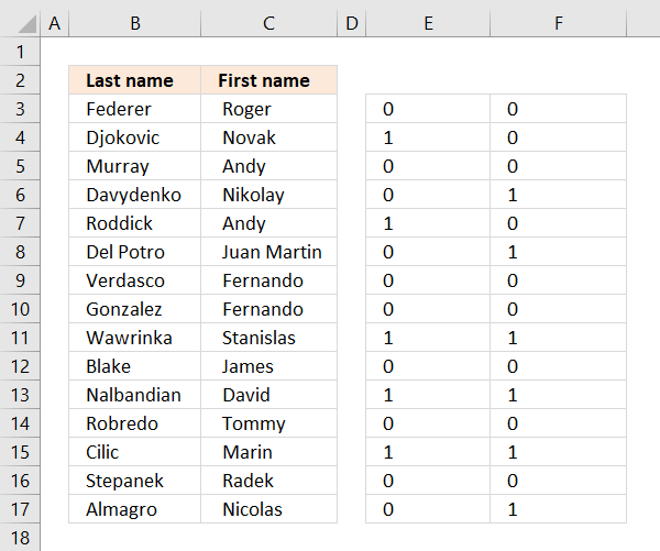
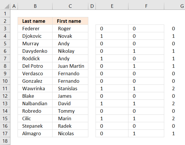
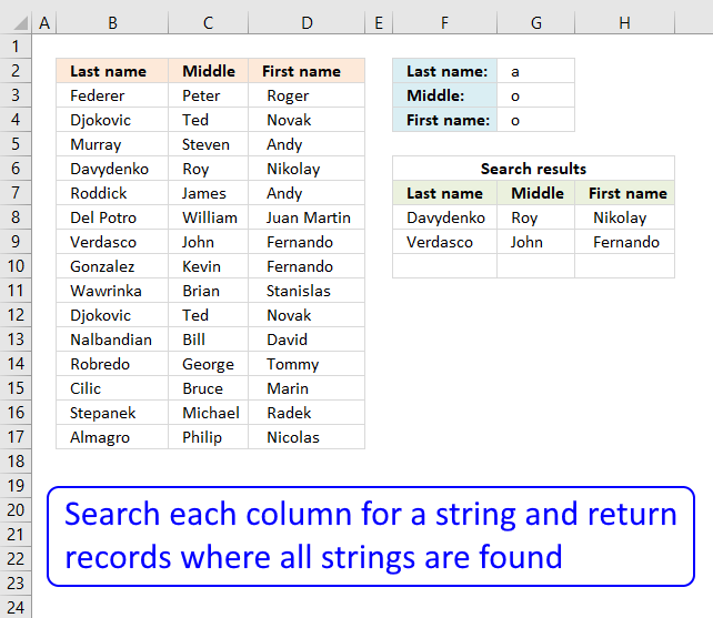
12. Search each column for a string each and return multiple records - OR logic
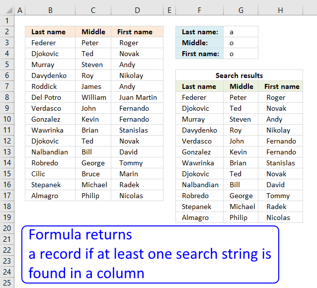
Can you please suggest if i want to find out the rows with fixed value in "First Name" but, if either of the criteria for "Middle Name" or "Last Name" will suffice. Also, i don't want repeated values in the final sheet.
For eg:
FN: a
MN: o
LN: o
Then, Davydenko Roy Nikolay should come only once.
Answer:
Excel 365 dynamic array formula:
Older Excel versions, array formula in cell F8:
How to create an array formula
- Copy (Ctrl + c) and paste (Ctrl + v) array formula into formula bar. See picture below.
- Press and hold Ctrl + Shift.
- Press Enter once.
- Release all keys.

How to copy array formula
- Copy (Ctrl + c) cell E9
- Paste (Ctrl + v) array formula on cell range E9:G11
Explaining formula in cell F8
Step 1 - Search for criteria
The SEARCH function allows you to find a string in a cell and it's position. It also allows you to search for multiple strings in multiple cells if you arrange values in a way that works. That is why I use the TRANSPOSE function to transpose the values.
SEARCH(TRANSPOSE($G$2:$G$4), $B$3:$D$17)
becomes
SEARCH(TRANSPOSE({"a"; "o"; "o"}), $B$3:$D$17)
becomes
SEARCH(TRANSPOSE({"a"; "o"; "o"}), {"Federer", "Peter", " Roger ";"Djokovic", "Ted", " Novak ";"Murray", "Steven", " Andy ";"Davydenko", "Roy", " Nikolay ";"Roddick", "James", " Andy ";"Del Potro", "William", " Juan Martin ";"Verdasco", "John", " Fernando ";"Gonzalez", "Kevin", " Fernando ";"Wawrinka", "Brian", " Stanislas ";"Blake", "Ted", " James ";"Nalbandian", "Bill", " David ";"Robredo", "George", " Tommy ";"Cilic", "Bruce", " Marin ";"Stepanek", "Michael", " Radek ";"Almagro", "Pihilip", " Nicolas "})
and returns
{#VALUE!, #VALUE!, 3;#VALUE!, #VALUE!, 3;5, #VALUE!, #VALUE!;2, 2, 5;#VALUE!, #VALUE!, #VALUE!;#VALUE!, #VALUE!, #VALUE!;5, 2, 9;5, #VALUE!, 9;2, #VALUE!, #VALUE!;3, #VALUE!, #VALUE!;2, #VALUE!, #VALUE!;#VALUE!, 3, 3;#VALUE!, #VALUE!, #VALUE!;5, #VALUE!, #VALUE!;1, #VALUE!, 5}.
Step 2 - Convert numbers to true
The ISNUMBER function returns TRUE if value is a number and FALSE for everything else even errors which is very handy in this case, the search function returns #VALUE! error if a string is not found in a particular cell.
--(ISNUMBER(SEARCH(TRANSPOSE($G$2:$G$4), $B$3:$D$17)))
becomes
--(ISNUMBER({#VALUE!, #VALUE!, 3;#VALUE!, #VALUE!, 3;5, #VALUE!, #VALUE!;2, 2, 5;#VALUE!, #VALUE!, #VALUE!;#VALUE!, #VALUE!, #VALUE!;5, 2, 9;5, #VALUE!, 9;2, #VALUE!, #VALUE!;3, #VALUE!, #VALUE!;2, #VALUE!, #VALUE!;#VALUE!, 3, 3;#VALUE!, #VALUE!, #VALUE!;5, #VALUE!, #VALUE!;1, #VALUE!, 5}))
becomes
--({FALSE, FALSE, TRUE;FALSE, FALSE, TRUE;TRUE, FALSE, FALSE;TRUE, TRUE, TRUE;FALSE, FALSE, FALSE;FALSE, FALSE, FALSE;TRUE, TRUE, TRUE;TRUE, FALSE, TRUE;TRUE, FALSE, FALSE;TRUE, FALSE, FALSE;TRUE, FALSE, FALSE;FALSE, TRUE, TRUE;FALSE, FALSE, FALSE;TRUE, FALSE, FALSE;TRUE, FALSE, TRUE})
The MMULT function can't work with boolean values so we need to convert them into their numerical equivalents. TRUE - 1 annd FALSE - 0 (zero).
--({FALSE, FALSE, TRUE;FALSE, FALSE, TRUE;TRUE, FALSE, FALSE;TRUE, TRUE, TRUE;FALSE, FALSE, FALSE;FALSE, FALSE, FALSE;TRUE, TRUE, TRUE;TRUE, FALSE, TRUE;TRUE, FALSE, FALSE;TRUE, FALSE, FALSE;TRUE, FALSE, FALSE;FALSE, TRUE, TRUE;FALSE, FALSE, FALSE;TRUE, FALSE, FALSE;TRUE, FALSE, TRUE})
and returns
{0, 0, 1;0, 0, 1;1, 0, 0;1, 1, 1;0, 0, 0;0, 0, 0;1, 1, 1;1, 0, 1;1, 0, 0;1, 0, 0;1, 0, 0;0, 1, 1;0, 0, 0;1, 0, 0;1, 0, 1}
Step 3 - Sum values row-wise
MMULT(--(ISNUMBER(SEARCH(TRANSPOSE($G$2:$G$4), $B$3:$D$17))), {1;1;1})
becomes
MMULT({0, 0, 1;0, 0, 1;1, 0, 0;1, 1, 1;0, 0, 0;0, 0, 0;1, 1, 1;1, 0, 1;1, 0, 0;1, 0, 0;1, 0, 0;0, 1, 1;0, 0, 0;1, 0, 0;1, 0, 1}, {1;1;1})
and returns
{1; 1; 1; 3; 0; 0; 3; 2; 1; 1; 1; 2; 0; 1; 2}
Step 4 - Convert non-numerical values to corresponding row numbers
The following IF function returns the row number if number is above 0 (zero), there are three strings that must match. FALSE returns "" (nothing).
IF(MMULT(--(ISNUMBER(SEARCH(TRANSPOSE($G$2:$G$4), $B$3:$D$17))), {1; 1; 1})>0, MATCH(ROW($B$3:$D$17), ROW($B$3:$D$17)), "")
becomes
IF({1; 1; 1; 3; 0; 0; 3; 2; 1; 1; 1; 2; 0; 1; 2}>0, MATCH(ROW($B$3:$D$17), ROW($B$3:$D$17)), "")
becomes
IF({1; 1; 1; 3; 0; 0; 3; 2; 1; 1; 1; 2; 0; 1; 2}>0, {1; 2; 3; 4; 5; 6; 7; 8; 9; 10; 11; 12; 13; 14; 15}, "")
and returns
{1;2;3;4; "";"";7; 8;9;10; 11;12; "";14;15}.
Step 5 - Extract k-th smallest value in array
The SMALL function makes sure that a new value is returned in each row.
SMALL(IF(MMULT(--(ISNUMBER(SEARCH(TRANSPOSE($G$2:$G$4), $B$3:$D$17))), {1; 1; 1})>0, MATCH(ROW($B$3:$D$17), ROW($B$3:$D$17)), ""), ROWS($A$1:A1))
becomes
SMALL({1;2;3;4; "";"";7; 8;9;10; 11;12; "";14;15}, ROWS($A$1:A1))
The ROWS function returns a new number because the cell reference expands as the formula is copied to cells below.
SMALL({1;2;3;4; "";"";7; 8;9;10; 11;12; "";14;15}, ROWS($A$1:A1))
becomes
SMALL({1;2;3;4; "";"";7; 8;9;10; 11;12; "";14;15}, 1)
and returns 1.
Step 6 - Return value
The INDEX function returns a value based on a row and column number.
INDEX($B$3:$D$17, SMALL(IF(MMULT(--(ISNUMBER(SEARCH(TRANSPOSE($G$2:$G$4), $B$3:$D$17))), {1; 1; 1})=3, MATCH(ROW($B$3:$D$17), ROW($B$3:$D$17)), ""), ROWS($A$1:A1)), COLUMNS($A$1:A1))
becomes
INDEX($B$3:$D$17, 1, COLUMNS($A$1:A1))
becomes
INDEX($B$3:$D$17, 1, 1)
and returns "Federer" in cell F8.
Get Excel *.xlsx file
multiple-criteria-lookup-with-multiple-unique-results-OR-LOGIC.xlsx
13. How to extract rows containing digits
This section describes formulas that returns all rows containing at least one digit 0 (zero) to 9.
What's on this section
- Question
- Filter rows containing at least one digit in any cell on the same row (Array formula)
- Filter rows containing at least one digit in any cell on the same row (Excel 365 formula)
- Filter rows containing at least one digit in any cell on the same row (Formula and an Excel Table)
- Get the Excel File here
Hello Oscar,
What code is needed to cause cells in Columns F - I to fill with the contents of Columns C - E when a cell in Column B includes a numeric value?
Answer:
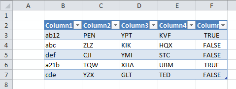
The data set above contains random characters, some of the cells in column B contain numeric values, as well.
13.1. Filter rows containing at least one digit in any cell on the same row

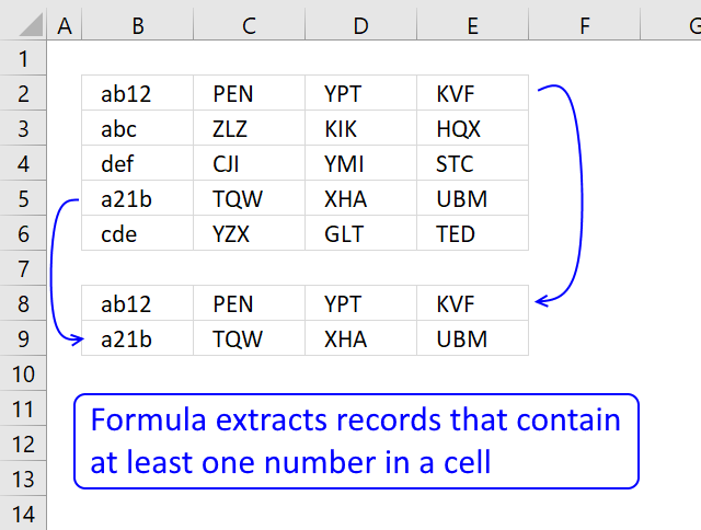
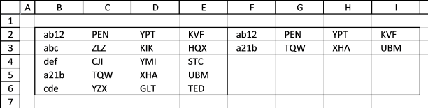
Cell range B2:E6 contains random values, the formula in cell B8 extracts rows from B2:E6 if the corresponding value in cells B2:B6 contains a number.
Array formula in cell F2:
The formula in cell B8 extracts rows from B2:E2 and B5:E5, they all have numbers in cells B2 and B5.
13.1.1 How to enter an array formula
- Copy formula above
- Doublepress with left mouse button on cell F2
- Paste formula
- Press and hold CTRL + SHIFT
- Press Enter
If you did this correctly, the formula in the formula bar now begins with a curly bracket and ends with a curly bracket, like this: {=formula}
Don't enter these curly brackets yourself, they will appear if you did the above steps.
Copy cell F2 and paste to cell range F2:I6.
13.1.2 Explaining array formula in cell F2
Step 1 - Look for values in a cell range
The SEARCH function returns the number of the character at which a specific character or text string is found reading left to right (not case-sensitive)
Function syntax: SEARCH(find_text,within_text, [start_num])
SEARCH({1, 2, 3, 4, 5, 6, 7, 8, 9, 0}, $B$2:$B$6)
becomes
SEARCH({1, 2, 3, 4, 5, 6, 7, 8, 9, 0}, {"ab12"; "abc"; "def"; "a21b"; "cde"})
and returns this array:
Step 2 - Remove errors
The IFERROR function if the value argument returns an error, the value_if_error argument is used. If the value argument does NOT return an error, the IFERROR function returns the value argument.
Function syntax: IFERROR(value, value_if_error)
IFERROR(SEARCH({1, 2, 3, 4, 5, 6, 7, 8, 9, 0}, $B$2:$B$6), 0)
returns
Step 3 - Return the matrix product of two arrays
The ROW function calculates the row number of a cell reference.
Function syntax: ROW(reference)
ROW($A$1:$A$10) returns {1; 2; 3; 4; 5; 6; 7; 8; 9; 10}
The MMULT function calculates the matrix product of two arrays, an array as the same number of rows as array1 and columns as array2.
Function syntax: MMULT(array1, array2)
MMULT(IFERROR(SEARCH({1, 2, 3, 4, 5, 6, 7, 8, 9, 0}, $B$2:$B$6), 0), ROW($A$1:$A$10))
returns {11;0;0;7;0}
Step 4 - Check whether a condition is met
The MATCH function returns the relative position of an item in an array that matches a specified value in a specific order.
Function syntax: MATCH(lookup_value, lookup_array, [match_type])
MATCH(ROW($B$2:$B$6), ROW($B$2:$B$6)) returns {1;2;3;4;5}
The IF function returns one value if the logical test is TRUE and another value if the logical test is FALSE.
Function syntax: IF(logical_test, [value_if_true], [value_if_false])
IF(MMULT(IFERROR(SEARCH({1, 2, 3, 4, 5, 6, 7, 8, 9, 0}, $B$2:$B$6), 0), ROW($A$1:$A$10)), MATCH(ROW($B$2:$B$6), ROW($B$2:$B$6)), "")
returns {1;"";"";4;""}
Step 5 - Return the k-th smallest value in array
The SMALL function returns the k-th smallest value from a group of numbers.
Function syntax: SMALL(array, k)
SMALL(IF(MMULT(IFERROR(SEARCH({1, 2, 3, 4, 5, 6, 7, 8, 9, 0}, $B$2:$B$6), 0), ROW($A$1:$A$10)), MATCH(ROW($B$2:$B$6), ROW($B$2:$B$6)), ""), ROWS($A$1:A1))
becomes
SMALL({1;"";"";4;""}, ROWS($A$1:A1))
becomes
SMALL({1;"";"";4;""}, 1)
and returns 1.
The ROWS function calculate the number of rows in a cell range.
Function syntax: ROWS(array)
Step 6 - Return a value of the cell at the intersection of a particular row and column
The INDEX function returns a value or reference from a cell range or array, you specify which value based on a row and column number.
Function syntax: INDEX(array, [row_num], [column_num])
INDEX($B$2:$E$6, SMALL(IF(MMULT(IFERROR(SEARCH({1, 2, 3, 4, 5, 6, 7, 8, 9, 0}, $B$2:$B$6), 0), ROW($A$1:$A$10)), MATCH(ROW($B$2:$B$6), ROW($B$2:$B$6)), ""), ROWS($A$1:A1)), COLUMNS($A$1:A1))
returns ab12 in cell F2.
13.2. Filter rows containing at least one digit in any cell on the same row (Excel 365 formula)

The image above demonstrates a dynamic array formula that works only in Excel 365, it spills it 's values to cell B8 and adjacent cells as far as needed.
Cell range B2:E6 contains random values, the formula in cell B8 extracts rows from B2:E6 if the corresponding value in cells B2:B6 contains a number.
Excel 365 formula in cell B8:
The formula in cell B8 extracts rows from B2:E2 and B5:E5, they all have numbers in cells B2 and B5. Here is a short breakdown of the formula:
- SEARCH({1, 2, 3, 4, 5, 6, 7, 8, 9, 0}, B2:B6): Search for digits 0 to 9 in cell range B2:B6. This creates an array that has 10 columns and 5 rows. If a digit is not found an #VALUE! error is returned, if found a number representing the starting position is returned.
- IFERROR(SEARCH({1, 2, 3, 4, 5, 6, 7, 8, 9, 0}, $B$2:$B$6), 0) : This catches all errors and returns 0 instead.
- SEQUENCE(10): This creates a sequence from 1 to 10, as many as there are numbers which is always 10.
- MMULT(IFERROR(SEARCH({1, 2, 3, 4, 5, 6, 7, 8, 9, 0}, $B$2:$B$6), 0), SEQUENCE(10)): This step adds all the numbers per row creating a vertical array. Each number in the array corresponds to each row in the source data range. If no numbers are found 0 (zero) is returned for a particular row. A number greater than 0 (zero) is returned if a number is found.
- FILTER(B2:E6, MMULT(IFERROR(SEARCH({1, 2, 3, 4, 5, 6, 7, 8, 9, 0}, $B$2:$B$6), 0), SEQUENCE(10))) : Filter rows that contain numbers. 0 (zero) equals FALSE and any other number equals TRUE.
13.3. Filter rows containing at least one digit in any cell on the same row (Formula and an Excel Table)

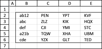
The image below shows the data table before it is converted to an Excel Table.
If you rather want to use an excel table filter, follow these instructions
- Select data set, cell range B2:E6
- Go to tab "Insert" on the ribbon
- Press with left mouse button on "Table" button or press CTRL + T
- Press with left mouse button on OK
- Double press with left mouse button on cell F2
- Type: =COUNT(FIND({0,1,2,3,4,5,6,7,8,9},B3))>0
- Press Enter
- Press with mouse on black arrow on Column 5 (F)
- Filter "True"
- Press with left mouse button on OK
Filter records containing a valuev3
14. How to extract email addresses from an Excel sheet
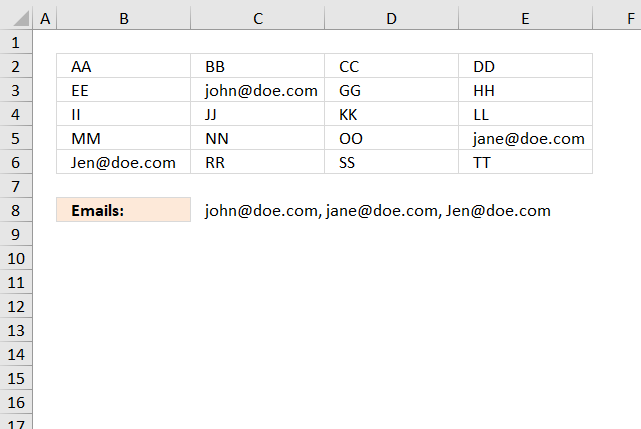
Question: How to extract email addresses from this sheet?
Answer:
It depends on how the emails are populated in your worksheet?
- Are they in a single cell each?
- Are there other text strings in the cell as well?
14.1. Example 1,
The following formula works if a cell contains only an email address, see image above. The TEXTJOIN function extracts all emails based on if character @ is found in the cell.
Array formula in cell C8:

Excel 365 formula in cell B9:
Explaining formula
Step 1 - Rearrange array to a single column array
The TOCOL function rearranges values in 2D cell ranges to a single column.
Function syntax: TOCOL(array, [ignore], [scan_by_col])
TOCOL(B2:E6)
returns {"AA"; "BB"; "CC"; ... ; "TT"}
Step 2 - Search for character @
The SEARCH function returns the number of the character at which a specific character or text string is found reading left to right (not case-sensitive)
Function syntax: SEARCH(find_text,within_text, [start_num])
SEARCH("@",TOCOL(B2:E6))
returns
{#VALUE!; #VALUE!; #VALUE!; ... ; #VALUE!}
Step 3 - Look for numbers
The ISNUMBER function checks if a value is a number, returns TRUE or FALSE.
Function syntax: ISNUMBER(value)
ISNUMBER(SEARCH("@",TOCOL(B2:E6)))
returns {FALSE; FALSE; FALSE; ... ; FALSE}
Step 4 - Filter values based on corresponding boolean values
The FILTER function extracts values/rows based on a condition or criteria.
Function syntax: FILTER(array, include, [if_empty])
FILTER(TOCOL(B2:E6),ISNUMBER(SEARCH("@",TOCOL(B2:E6))))
returns
{"[email protected]";"[email protected]";"[email protected]"}
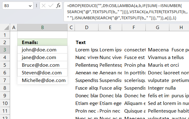
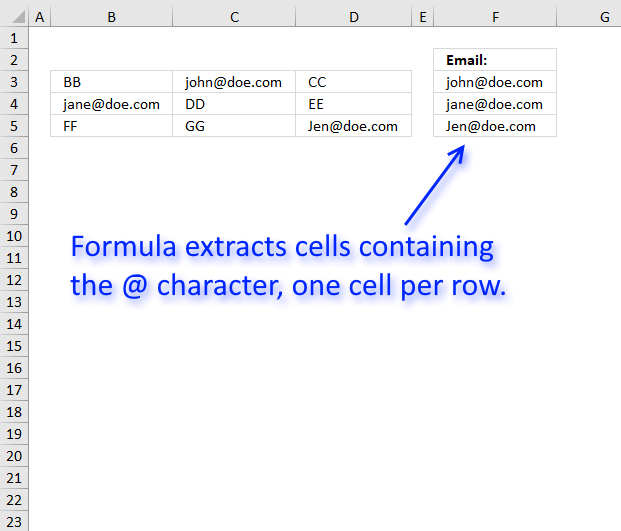
14.2 Example 2,
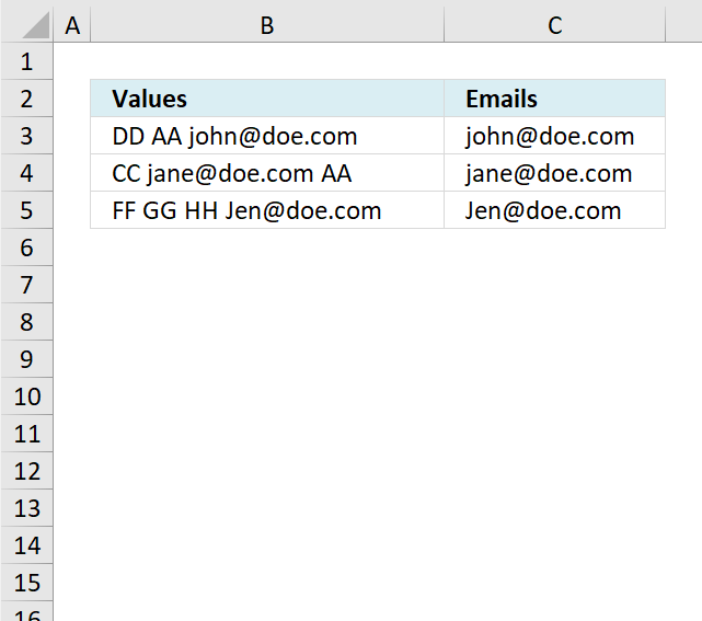
The example above has multiple text strings in each cell separated by a blank, the formula is only capable of extracting one email address per cell and if the delimiting character is a blank (space). You can change the formula to use any delimiting character, however, only one delimiting character per formula.
Formula in cell C3:

Excel 365 formula in cell D3:
Explaining formula
Step 1 - Merge strings in multiple cells
The TEXTJOIN function combines text strings from multiple cell ranges.
Function syntax: TEXTJOIN(delimiter, ignore_empty, text1, [text2], ...)
TEXTJOIN(" ",TRUE, B3:B5)
returns
"DD AA [email protected] CC [email protected] AA FF GG HH [email protected]"
Step 2 - Split strings based on a space character as a delimiting value
The TEXTSPLIT function splits a string into an array based on delimiting values.
Function syntax: TEXTSPLIT(Input_Text, col_delimiter, [row_delimiter], [Ignore_Empty])
TEXTSPLIT(TEXTJOIN(" ",TRUE, B3:B5),," ")
returns {"DD"; "AA"; "[email protected]"; "CC"; "[email protected]"; "AA"; "FF"; "GG"; "HH"; "[email protected]"}.
Step 3 - Search for a @ character
The SEARCH function returns the number of the character at which a specific character or text string is found reading left to right (not case-sensitive)
Function syntax: SEARCH(find_text,within_text, [start_num])
SEARCH("@",TEXTSPLIT(TEXTJOIN(" ",TRUE, B3:B5),," "))
returns {#VALUE!; #VALUE!; 5; .. ; 4}.
Step 4 - Find numbers in array
The ISNUMBER function checks if a value is a number, returns TRUE or FALSE.
Function syntax: ISNUMBER(value)
ISNUMBER(SEARCH("@",TEXTSPLIT(TEXTJOIN(" ",TRUE, B3:B5),," ")))
returns {FALSE; FALSE; TRUE; ... ; TRUE}.
Step 5 - Filter values based on correpsonding boolean array
The FILTER function extracts values/rows based on a condition or criteria.
Function syntax: FILTER(array, include, [if_empty])
FILTER(TEXTSPLIT(TEXTJOIN(" ",TRUE, B3:B5),," "),ISNUMBER(SEARCH("@",TEXTSPLIT(TEXTJOIN(" ",TRUE, B3:B5),," "))))
returns {"[email protected]";"[email protected]";"[email protected]"}.
Step 6 - Shorten formula
The LET function lets you name intermediate calculation results which can shorten formulas considerably and improve performance.
Function syntax: LET(name1, name_value1, calculation_or_name2, [name_value2, calculation_or_name3...])
FILTER(TEXTSPLIT(TEXTJOIN(" ",TRUE, B3:B5),," "),ISNUMBER(SEARCH("@",TEXTSPLIT(TEXTJOIN(" ",TRUE, B3:B5),," "))))
TEXTSPLIT(TEXTJOIN(" ",TRUE, B3:B5),," ") is repeated twice in the formula, lets name it x. The formula becomes:
LET(x,TEXTSPLIT(TEXTJOIN(" ",TRUE, B3:B5),," "),FILTER(x,ISNUMBER(SEARCH("@",x))))
14.3. Example 3,
It is possible to combine the array formulas in example 1 and 2, unfortunately, the formula can still only extract one email address per cell.
Array formula in cell B6:
Cell B6 has "Wrap text" enabled, select cell B6 and press CTRL + 1 to open the "Format Cells" dialog box.

14.4. Example 4,
If you need an even better faster formula I recommend using a UDF:
Recommended articles
This post describes ways to extract all matching strings from cells in a given cell range if they contain a […]
14.5 Example 5,
The formula in cell F3 gets only one email address per row so it is very basic, however, check out the comments for more advanced formulas.
If the cell contains an email address and also other text strings it won't extract the email only, as I said, it is a very basic formula.
Array formula in F3:
To enter an array formula, type the formula in cell F3 then press and hold CTRL + SHIFT simultaneously, now press Enter once. Release all keys.
 The formula bar now shows the formula with a beginning and ending curly bracket telling you that you entered the formula successfully.
Don't enter the curly brackets yourself, they appear automatically.
This article demonstrates how to filter emails with a custom function:
Recommended articles
This post describes ways to extract all matching strings from cells in a given cell range if they contain a […]
Explaining formula in cell F3
Step 1 - Look for @ character in cell range
The SEARCH function allows you to find the character position of a substring in a text string, we are, however, not interested in the position only if it exists or not in the cell.
SEARCH("@", B3:D3))
becomes
SEARCH("@", {"BB","[email protected]","CC"}))
and returns {#VALUE!,5,#VALUE!}. This tells us that the second value in the array contains a @ character on position 5.
Step 2 - Convert array to TRUE or FALSE
The IF function can't handle error values in the logical expression so we must first convert the array to boolean values. The ISERROR function returns TRUE if the value is an error value and FALSE if not.
ISERROR(SEARCH("@", B3:D3))
becomes
ISERROR({#VALUE!,5,#VALUE!})
and returns {TRUE,FALSE,TRUE}.
Step 3 - Return column number if value is not an error value
IF(ISERROR(SEARCH("@", B3:D3)), "", MATCH(COLUMN(B3:D3), COLUMN(B3:D3)))
To create an array from 1 to n I use the MATCH function and COLUMN function.
returns {"", 2,""}
Step 4 - Return the smallest column number
The MIN function calculates the smallest number in cell range or array.
MIN(IF(ISERROR(SEARCH("@", B3:D3)), "", MATCH(COLUMN(B3:D3), COLUMN(B3:D3))))
becomes MIN({"", 2,""})
and returns 2.
Step 4 - Return value corresponding to column number
The INDEX function returns a value based on a row and/or column number.
INDEX(B3:D3, MIN(IF(ISERROR(SEARCH("@", B3:D3)), "", MATCH(COLUMN(B3:D3), COLUMN(B3:D3)))))
becomes INDEX(B3:D3, 2)
and returns "[email protected]".
Get Excel *.xlsx file
15. Filter words containing a given string in a cell range - Excel 365 LAMBDA function
The cells in the specified range contain strings separated by a delimiter of your choice, with space being used as an example here to split strings in a cell value. This operation is performed on all cells mentioned in the argument.
The objective is to extract and return strings that contain a specific substring, denoted by the "@" character in this example.
Excel 365 LAMBDA function in cell B3:
Change @ in the formula above to whatever search string you want to find. Also change " " in TEXTSPLIT(b,," ") to change the delimiter if you don't want to use the space character. Perhaps you want to split strings by a comma, semicolon or a new row. Use char(10) to find new rows.
Explaining formula
Step 1 -
16. Filter words containing a given string in a cell range - UDF
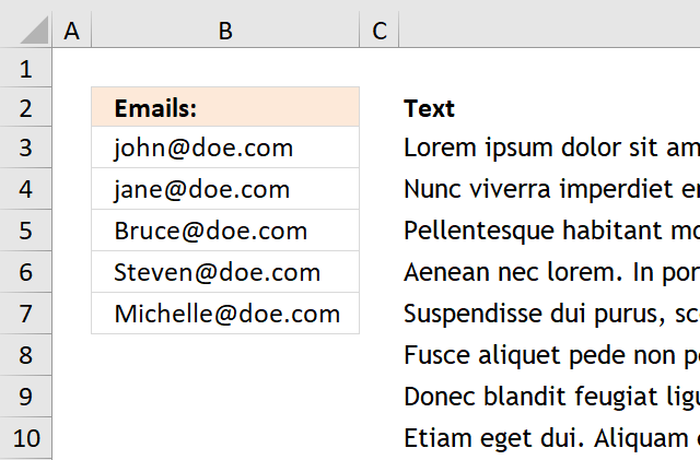
The image above demonstrates a User Defined Function that extracts all words containing a given string that you can specify. In this case it is a @ sign. A User Defined Function is a custom function that you can build yourself in the visual basic editor.
Example, cell range B1:M50 contains random sentences, I have inserted some random emails in this range, see image above.
Array formula in cell range B3:B7:
To enter an array formula, type the formula in a cell then press and hold CTRL + SHIFT simultaneously, now press Enter once. Release all keys.
The formula bar now shows the formula with a beginning and ending curly bracket telling you that you entered the formula successfully. Don't enter the curly brackets yourself.
VBA code
'Name function
Function FilterWords(rng As Range, str As String) As Variant()
'Declare variables
Dim x As Variant, Wrds() As Variant, Cells_row As Long
Dim Cells_col As Long, Words As Long, y() As Variant
'Redimension variable
ReDim y(0)
'Save values in range to array variable
Wrds = rng.Value
'Iterate through array variable
For Cells_row = LBound(Wrds, 1) To UBound(Wrds, 1)
  For Cells_col = LBound(Wrds, 2) To UBound(Wrds, 2)
    'Extract words in cell to an array
    x = Split(Wrds(Cells_row, Cells_col))
      'Iterate through word array
      For Words = LBound(x) To UBound(x)
        'Check if value in array is equal to the given string
        If InStr(x(Words), str) Then
          'Save value to another array
          y(UBound(y)) = x(Words)
          'Increase containers in array by 1
          ReDim Preserve y(UBound(y) + 1)
        End If
      Next Words
  Next Cells_col
Next Cells_row
'Decrease containers in array by 1
ReDim Preserve y(UBound(y) - 1)
'Return array
FilterWords = Application.Transpose(y)
End Function
Where to do I copy the code?
- Press Alt-F11 to open visual basic editor
- Press with left mouse button on Module on the Insert menu
- Copy and paste the user defined function to module
- Exit visual basic editor
17. Filter unique distinct strings from a cell range - Excel 365

Excel 365 dynamic array formula in cell D3:
Explaining formula in cell D3
Step 1 - Split cell values based on a delimiting space character
The TEXTSPLIT function splits a string into an array based on delimiting values.
Function syntax: TEXTSPLIT(Input_Text, col_delimiter, [row_delimiter], [Ignore_Empty])
TEXTSPLIT(x, , " ", 1)
Step 2 - Stack arrays vertically
The VSTACK function combines cell ranges or arrays. Joins data to the first blank cell at the bottom of a cell range or array (vertical stacking)
Function syntax: VSTACK(array1,[array2],...)
VSTACK(TEXTSPLIT(x, , " ", 1), TEXTSPLIT(y,, " ", 1))
Step 3 - A LAMBDA function is required with the REDUCE function
The LAMBDA function build custom functions without VBA, macros or javascript.
Function syntax: LAMBDA([parameter1, parameter2, …,] calculation)
LAMBDA(x, y, VSTACK(TEXTSPLIT(x, , " ", 1), TEXTSPLIT(y,, " ", 1)))
Step 4 - Send cell values to LAMBDA function
The REDUCE function shrinks an array to an accumulated value, a LAMBDA function is needed to properly accumulate each value in order to return a total.
Function syntax: REDUCE([initial_value], array, lambda(accumulator, value))
REDUCE(, B3:B15, LAMBDA(x, y, VSTACK(TEXTSPLIT(x, , " ", 1), TEXTSPLIT(y,, " ", 1))))
Step 5 - Extract unique distinct strings
The UNIQUE function returns a unique or unique distinct list.
Function syntax: UNIQUE(array,[by_col],[exactly_once])
UNIQUE(REDUCE(, B3:B15, LAMBDA(x, y, VSTACK(TEXTSPLIT(x, , " ", 1), TEXTSPLIT(y,, " ", 1)))))
18. Filter unique distinct strings from a cell range - UDF
This section describes how to create a list of unique distinct strings from a cell range. Unique distinct words are all strings but duplicate strings are only listed once.

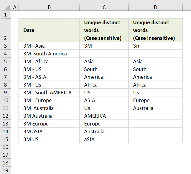
Cell range A2:A14 contains values, see the picture above. Values are split into strings using the space character as a delimiter. For example, the value in cell A2 is "3M - Asia". The value becomes the following strings: "3M", "-", and "Asia". Three strings in total.
Now consider all values in cell range A2:A14, some strings will be duplicates and some not.
Rick Rothstein (MVP - Excel) helped me out here with a powerful user defined function (udf).

Array formula in cell B2:B23
=ListOfWords($A$2:$A$18, TRUE) + CTRL + SHIFT + ENTER
Select all the cells to be filled, then type the above formula into the Formula Bar and press CTRL+SHIFT+ENTER
Array formula in cell C2:C23
=ListOfWords($A$2:$A$18, FALSE) + CTRL + SHIFT + ENTER
Select all the cells to be filled, then type the above formula into the Formula Bar and press CTRL+SHIFT+ENTER
User defined function

Instructions
- You can select far more cells to load the formulas in than are required by the list. The empty text string will be displayed for cells not having an entry.
- You can specify a larger range than the there are filled in cells as the argument to these macros to allow for future entries in the column.
- You can specify whether the listing is to be case sensitive or not via the optional second argument with the default value being FALSE, meaning duplicated entries with different casing like One, one, ONE, onE, etc.. will all be treated as if they were the same word with the same spelling. If you pass TRUE for that optional second argument, then those words would all be treated as if they were different words.
- For all the "Case Insensitive" listing, the words are listed in Proper Case (first letter upper case, remaining letters lower case). The reason being if you had One, one and ONE then there is not reason to prefer one version over another, so I solved the problem by using Proper Case throughout.
VBA Code:
Function ListOfWords(Rng As Range, Optional CaseSensitive As Boolean) As Variant
Dim X As Long, Index As Long, List As String, Words() As String, LoW As Variant
With WorksheetFunction
Words = Split(.Trim(Replace(Join(.Transpose(Rng)), Chr(160), " ")))
LoW = Split(Space(.Max(UBound(Words), Application.Caller.Count) + 1))
For X = 0 To UBound(Words)
If InStr(1, Chr(1) & List & Chr(1), Chr(1) & Words(X) & Chr(1), 1 - Abs(CaseSensitive)) = 0 Then
List = List & Chr(1) & Words(X)
If CaseSensitive Then
LoW(Index) = Words(X)
Else
LoW(Index) = StrConv(Words(X), vbProperCase)
End If
Index = Index + 1
End If
Next
ListOfWords = .Transpose(LoW)
End With
End Function
How to copy above code to your workbook
- Press Alt-F11 to open visual basic editor
- Press with left mouse button on Module on the Insert menu
- Copy and paste above user defined function to code module
- Exit visual basic editor
- Select a sheet
- Select a cell range
- Type =ListOfWords($A$2:$A$18, TRUE) into formula bar and press CTRL+SHIFT+ENTER
Get Rick Rothstein´s excel example file
Many thanks to Rick Rothstein (Mvp - Excel)!!
Filter records category
This article demonstrates how to extract records/rows based on two conditions applied to two different columns, you can easily extend […]
Lookup with criteria and return records.
This article presents methods for filtering rows in a dataset based on a start and end date. The image above […]
Excel categories
216 Responses to “Search for a text string in a data set and return multiple records”
Leave a Reply
How to comment
How to add a formula to your comment
<code>Insert your formula here.</code>
Convert less than and larger than signs
Use html character entities instead of less than and larger than signs.
< becomes < and > becomes >
How to add VBA code to your comment
[vb 1="vbnet" language=","]
Put your VBA code here.
[/vb]
How to add a picture to your comment:
Upload picture to postimage.org or imgur
Paste image link to your comment.
How would I go about looking up data in an cross ref table.
I have the header row (i.e. 24) value and the column (mm) value and want to return the x/y value. i.e I have 25/X and 9/Y item and want 1.8 to be returned.
(mm) 22 23 24 25 26 27 28 29
8 1.3 1.8 1.8 1.8 1.8 1.8 2.3 2.3
9 1.3 1.8 1.8 1.8 1.8 1.8 2.3 2.3
10 1.3 1.8 1.8 1.8 1.8 1.8 2.3 2.3
11 2.2 2.8 2.8 2.8 2.8 2.8 3.3 3.3
thanks
See this post: https://www.get-digital-help.com/looking-up-data-in-a-cross-reference-table-in-excel/
Could this approach be expanded for more than 2 columns?
And if the values were numbers is there a way to display the values within a range between the values in 2 cells?
I don´t understand.
You want to search a range bigger than 2 columns?
If two numbers (or numbers between) match on any column on the same row, it is a match?
My comment is two seperate issues.
The first is if I can expand this equation set into more than two colums of data, say if I had a first, middle and last name column could I only display the values in which all three cases are true?
The second question is whether the equation can be adjusted to search and display a range of values, if the values were numerical, say 1 - 40 could I set a range of 20 - 25 (either in one or 2 cells) and get 6 values (inclusive)?
Apologies if it is hard to understand
Gavin, your first question.
See this blog post: https://www.get-digital-help.com/lookup-with-multiple-criteria-and-display-multiple-search-results-using-excel-formula-part-3/
Gavin, your second question:
https://www.get-digital-help.com/search-and-display-a-range-of-values-in-excel/
You are a genius. Formulas are simple, and easy to understand.
I have a column "A" with a last name.. I have another columb with a date in it "E"... I need to be able to list the names from columb A on a second sheet whos columb e date has past....
thanks
todd B, see this post: https://www.get-digital-help.com/list-names-whos-date-has-past-in-excel/
Well, I have been looking long for this wonderful idea, and previously I had to result in two step utilizing rank command etc etc..
Thank you for the work, and thenk the NET in general!
Back to what I had in mind, I wanted specificaly do this
assume a column b from 2 to 100, where the word "check" occures, there is dropdown list resticted option, among "cash" and "other".
next to it, there is a column c from 2 to 100 also with dates, Now all I want is to incorporate in that wonderful formula of yours for simple sorting, the condition to have value "check" on col b every time I include a date for to sort..and of course to include the option to have the cells blank when there is no value...after sorting..?
Thank you for your time, it has been so much fun doing stuff in excel!!!
am I asking for too much
also, while this formula modified for one constant filtration, either from small or family names lets say the "o" s, it does not alphabetize the results.
so what I am looking for is your classic short formula, single column, the one you have with pairs of letters...ee, wr, etc, but with a filter to screen the results too...
Is it possible to lets say pick the cell that is next to it horizontaly, and the cell next to it too, like the vlookup can do?
Ultimately I want to filtrate and indexize the dates, but also bring in the rest of the row, the name the ammount etc, associated with the date...
thank you once again
Can you upload an excel example file?
https://www.get-digital-help.com/contact/
Could this be done to filter for 10 criteria?
10 criteria in each column? 10 criteria in all columns?
Hi,
i had a similar query and i believe your example is the way forward for me but i can't get my search to work.
like your example i'm searching 3 columns but in a table of 8 colums and the search function is on a seperate tab. there is also a gap between the columns i'm searching. i also decided not to name the ranges as they may change. are any of the above affecting the formala or is it just me?
ignore my last comment... it works a treat!! (i put in one too many $ signs!!)
Thanks!
I second G's question: can this be done for more than 3?
i.e.
(Instead of last name, middle, first)
customer#, cust name, appt date, appt time, venue, coordinator, assistant
Thanks for putting this up!
D,
See this blog post: https://www.get-digital-help.com/lookup-with-multiple-criteria-and-display-multiple-search-results-using-excel-formula-part-4/
Thank you so much for this formula! You helped me so much. Please don't stop helping others. You certainly have a gift. God Bless!
Thanks Michael!
There seems to be an error in the above formula. If cell A11 contains the text value Million and B11 contains the text value Millio the formula returns TRUE.
(Thanks Niranjan)
Here is a formula that produces the same output as the one you posted but which uses less than half the number of function calls, is almost half the size (length-wise) and which produces the same output...
=AND(NOT(ISNUMBER(FIND(UPPER(MID("="&A2&"=", SEARCH(B2, A2), 1)), "ABCDEFGHIJKLMNOPQRSTUVWXYZ"))), NOT(ISNUMBER(FIND(UPPER(MID("="&A2&"=", FIND(UPPER(B2), UPPER(A2))+LEN(B2)+1, 1)), "ABCDEFGHIJKLMNOPQRSTUVWXYZ"))))
Note: I used the FIND/UPPER construction on purpose; if you used SEARCH then "exact words" lying next to an asterisk or question mark could make the formula produce incorrect results because SEARCH would assume they were wildcards.
By the way, if you missed it, I think you might be interested in the update John posted to his blog entry showing the one-liner VB function that I sent him which does the same thing as his 12-line function does.
CORRECTION...
Damn, I posted the wrong formula (it is missing the IF function housing. Here is the correct formula...
=IF(ISNUMBER(SEARCH(B2, A2)), AND(NOT(ISNUMBER(FIND(UPPER(MID("="&A2&"=", SEARCH(B2, A2), 1)), "ABCDEFGHIJKLMNOPQRSTUVWXYZ"))), NOT(ISNUMBER(FIND(UPPER(MID("="&A2&"=", SEARCH(B2, A2)+LEN(B2)+1, 1)), "ABCDEFGHIJKLMNOPQRSTUVWXYZ")))))
The comparison numbers change with this (one, because I had left some function calls out, but two, because I left the separating spaces in the function you posted)... my formula is about two-thirds the length of yours (215 characters versus 318 characters) and it uses just a little more than half the function calls (17 versus 31).
Amazing! Your formula works perfectly! Thank you for commenting!
You are quite welcome. When I first saw the question in John Walkenbach's blog, he had posted a VBA solution so I gave him back my one-liner VBA solution as a response. It did not even occur to me to try and solve the problem via a worksheet formula. When I saw your posted formula solution, it prompted me to try my hand at one as well. It was a fun exercise, so I thank you for thinking of it.
Now, back to your "Your formula works perfectly" comment. I just want to point out one difference between my formula and yours... as written, my formula is case **insensitive** where as yours is not. Walkenbach's original code was case insensitive, so I made my response to him the same... and it made sense to me for it to be case insensitive to cover the possibility that the word might be located at the beginning of a sentence. However, if you want to change my formula to be case sensitive, you can do that by simply changing the very first SEARCH function call to a FIND function call (leaving the rest of the formula alone).
Here's something I came up with to extract the email from an adjacent cell (called A1) of text(so put this formula in B1 and copy down). It assumes the email address has a blank space on either side within the body text.
=CONCATENATE(RIGHT(SUBSTITUTE(LEFT(A1,SEARCH("@",A1,1)-1)," "," ^!",(LEN(LEFT(A1,SEARCH("@",A1,1)-1))-LEN(SUBSTITUTE(LEFT(A1,SEARCH("@",A1,1)-1)," ","")))),(SEARCH("@",A1,1)-SEARCH("^!",SUBSTITUTE(LEFT(A1,SEARCH("@",A1,1)-1)," "," ^!",(LEN(LEFT(A1,SEARCH("@",A1,1)-1))-LEN(SUBSTITUTE(LEFT(A1,SEARCH("@",A1,1)-1)," ","")))),1))),MID(A1,SEARCH("@",A1,1),SEARCH(" ",A1,SEARCH("@",A1,1))-SEARCH("@",A1,1)))
Fred,
Your formula works! Thanks for sharing!
Thanks also for bringing this post to my attention. I have changed the array formula and the attached excel file.
Here is a much shorter formula to find the email address within a cell and it allows that email address to be anywhere within the text (beginning, middle or end)...
=TRIM(RIGHT(SUBSTITUTE(LEFT(A1,FIND("@",A1)-1)," ",REPT(" ",99)),99))&MID(A1,FIND("@",A1),FIND(" ",A1&" ",FIND("@",A1))-FIND("@",A1))
Rick Rothstein (MVP - Excel),
Your formula worked great.
Thanks
I get this to work but I have email with ( at beginning and ) at the end of the address how would I modify the formula to remove the () from the address?
worked for me too. thanks for sharing
Rick Rothstein (MVP - Excel),
Great formula, you got me thinking there for a while! Thanks for sharing!
I'm glad you were able to figure out how my formula (for finding an email address inside a text string) works. Here is a slightly different formula that does what you posted in your original blog entry (get the email address from whatever column it is in)...
=INDEX(A1:C1,1,MIN(IF(ISERR(SEARCH("@",A1:C1)),"",COLUMN(A1:C1))))
This formula, like the one you blogged, requires Ctrl+Shift+Enter to commit it.
Whoops! Sorry, I posted your blogged formula by mistake; here is the formula I meant to post...
=INDEX(1:1,,MAX(COLUMN(A1:C1)*NOT(ISERROR(SEARCH("@",A1:C1)))))
And again, for completeness sake, this formula, like the one you blogged, requires Ctrl+Shift+Enter to commit it.
Rick your formula works!!! so thankful to you!
I would like to use the "original" formula which is used in the example file. However it's case sensitive and I need it case insensitive as some of the words I'm looking for is the first letter and therefore Capital letter. Can you help with that.
Great solution. I was wondering, though, how you seemed to "group" the cells D6:D20 and E6:E20. I got the Excel example and played around and noticed that changing something in D6 automatically changed every cell from D6 to D20. That's cool!
Feel free to e-mail me if you prefer. Thanks!
Art,
I use search() to find rows that match. INDEX() returns a value in a given range.
The formula in D6:D20:
= INDEX($B$2:$B$16, ...
The formula in E6:E20:
= INDEX($A$2:$A$16, ...
Thanks for commenting!
/Oscar
I applied this in my spreadsheet and worked perfectly well.
However, I noticed that if a cell in the search range is blank, it does not include it in the results. In your example, if B2 was blank instead of having the value "Ted." that name would not show up in the search results (E9:E11).
Is there a work around for this? The spreadsheet I have may have blank cells but I need them to show in the results page.
Thanks!!!
I have a excel-document with some 2000 rows, with link to contacts details on the internet (where I can find e-mailaddresses) Is it possible to make a string that works for that?
No, I don´t think it is possible. But I believe you can use vba to search the html found at each http address.
A very quick method to extract email addresses is to use a text filter. Select the column with email addresses (and other info) and apply a text filter, using the 'contains' parameter, to filter on the '@' character. That will collapse all rows without an email address, allowing you to cut and past only the email addresses to another spreadsheet, or elsewhere.
Hi Terry! I came across this post by you. I'm just trying to figure out how to get email addresses out from a bunch of all other texts in excel but I'm really unfamiliar with it. Could you give me a more detailed step wise instruction on how to do it? Thanks for your help in advance!
Jun
Terry Wright,
I tried your method and it worked great!
Thanks for commenting!
Hi, this is a great formula. How can it be changed to detect whole numbers? Example String:
132, 98, 198, 200 - 222 AXT 78
Where if I search for 98 it returns TRUE but 22 returns FALSE.
Thanks for any help!
@Mario,
It is unclear if you are referring to my formula or the formula that Oscar included in his original blog article. Assuming you meant my function, I believe this modification of it will work correct to search for the specified number (and ONLY for numbers, not non-digits, even if coupled with digits) within a string of characters...
=IF(ISNUMBER(SEARCH(B2, A2)), AND(NOT(ISNUMBER(FIND(MID("="&A2&"=", SEARCH(B2, A2), 1), "0123456789"))), NOT(ISNUMBER(FIND(MID("="&A2&"=", SEARCH(B2, A2)+LEN(B2)+1, 1), "0123456789")))))
Any idea how to adapt the formula to do a conditional (i.e. comma-separated) merge of the data from multiple columns, in the case that a single row has emails spread over several columns?
I think I would need to change the MIN as it only pulls the first match out of the set of matched SEARCH values (i.e. anything containing an "@" symbol)... if anyone has an idea of a better function to use than MIN please let me know... my first inclination was to use CONCAT but didn't seem to work.
Well for starters it is CONCATENATE not CONCAT, but this thing is driving me nuts.... beer $ for anyone who solves it
Here's what I'm trying to do:
[email protected] | [email protected] | [email protected] | CONCATENATED LIST
The formula posted here only takes the first occurrence of an email in any column, I'd like to merge a comma-separated list of all the emails in separate columns (same row)
magneticone,
See this post: https://www.get-digital-help.com/filter-emails-spread-over-several-columns-in-excel/
Rick Rothstein - you have seriously saved my day.
@Mattias Olsson,
I'm not sure which of my two formulas you were referring to, unless you meant my macro (which I alluded to in my first response to Oscar) that John Walkenbach posted in his blog; but I just wanted to say that you are quite welcome, I am glad that something I posted turned out to be useful to you.
Thank you all for commenting!
Oscar, do you know of any macro or free files to calculate the processing speed of Excel formulas or functions?
I know you can use "Timer" to calculate user defined functions and macros. John Walkenbach has an example on his blog: How Fast Is Your System?
THis is great!!!
What if I want to search using 4 criteria? Can you please help me?
Thanks!
I notice that your UDF requires spaces to delimit the email address. For example, if the email address is surrounded by parentheses or adjacent to punctuation marks, those will remain attached to the returned email addresses. This is because you used a general word parser as the basis for your UDF. I had a robust email address parser function that I wrote awhile ago, so I wrote a front-end function (the UDF) that repeatedly calls it as needed; doing this makes the UDF return only the email addresses no matter what other delimiting characters surround them. Just copy the following two functions into a standard Module, then select a column of cells (more than you think email addresses exist), enter this formula in the Formula Bar (change the range as necessary)...
=FindEmailAddresses(B1:M50)
and then press CTRL+SHIFT+ENTER to commit the array formula. By the way, the GetEmailAddress function below can be used as a stand-alone function by itself... it returns a single email address (the first it finds in the text passed to it). Okay, here are the functions...
Function FindEmailAddresses(Rng As Range) As Variant()
Dim Temp As String, Cell As Range, EM() As Variant
ReDim EM(0)
For Each Cell In Rng
Temp = Cell.Value
Do While InStr(Temp, "@")
EM(UBound(EM)) = GetEmailAddress(Temp)
Temp = Replace(Temp, "@", "", 1, 1)
ReDim Preserve EM(UBound(EM) + 1)
Loop
Next
ReDim Preserve EM(UBound(EM) - 1)
FindEmailAddresses = WorksheetFunction.Transpose(EM)
End Function
Function GetEmailAddress(ByVal S As String) As String
Dim X As Long, AtSign As Long
Dim Locale As String, DomainPart As String
Locale = "[A-Za-z0-9.!#$%&'*/=?^_`{|}~+-]"
Domain = "[A-Za-z0-9._-]"
AtSign = InStr(S, "@")
For X = AtSign To 1 Step -1
If Not Mid(" " & S, X, 1) Like Locale Then
S = Mid(S, X)
If Left(S, 1) = "." Then S = Mid(S, 2)
Exit For
End If
Next
AtSign = InStr(S, "@")
For X = AtSign + 1 To Len(S) + 1
If Not Mid(S & " ", X, 1) Like Domain Then
S = Left(S, X - 1)
If Right(S, 1) = "." Then S = Left(S, Len(S) - 1)
GetEmailAddress = S
Exit For
End If
Next
End Function
Min,
I have changed the formula. I think the new formula is easier. I have also written an explanation, perhaps with help from explanation, you can now add a fourth criterion yourself? Otherwise, comment here again.
I uploaded a new file, as well.
Rick Rothstein (MVP - Excel),
Thank you for your valuable comment! I tried your functions and they work as you described!
Guys, just got the ASAP utilities, it can do what you talk about and much more, and it's free! (shareware if you are a business only)
Philippe
Hi,
Your articles are really helpful! Can you please suggest if i want to find out the rows with fixed value in "First Name" but, if either of the criteria for "Middle Name" or "Last Name" will suffice. Also, i don't want repeated values in the final sheet.
For eg:
FN: a
MN: o
LN: o
Then, Davydenko Roy Nikolay should come only once.
Regards
gr8..really thanksful Rick Rothstein
@tricky...
Thanks for commenting on my formulas; I am glad you found them useful to you in some way. If you are into VB code, you should check out my response to John Walkenbach... my one-liner VB code is even more compact than the formula version. See the *UPDATE* section on this webpage...
https://spreadsheetpage.com/index.php/tip/is_a_particular_word_contained_in_a_text_sring/
RU,
Read this post: Lookup with multiple criteria and display multiple unique search results (array formula)
This solution was elegant and consistent! The only issue I am facing, (or so I've been told by an associate) is that as the number of entries increases, it would be best to write this functionality into a module(?) for the sake of performance. Any ideas, solutiobns or resources would be appreciated!! Thank you!!
Jim,
I have added a custom function to this post. I have not done any performance testing.
Is is possible to use Index/Match using multiple criteria as you listed above except display all of the search results in a list (data validation) so that I can select one of the results from the list?
Hey Rick - You just saved me hours of manual work...hats off to you. Thanks..
Dear Oscar,
Do you know if there is a formula (or combination) that results in a text value I want to use with "vlookup"
Something like the "like" function in Access.
Example:
text = "Kn1263-Techstore-MrFixit-12-11-2011"
I want to Find the part "Tech".
Then with Vlookup I want to find a related account in an Table.
such a Tech is related to "200 Repare account"
So I can keep controle over my Bankaccount for example.
Maybe in VBA?
Thanks in advance for your reply.
Kind regards,
Lourens van 't Wout
The Netherlands
Lourens van 't Wout,
Yes, I believe it is possible.
Can you describe the two tables and how they are related?
Lourens,
This post describes how to search for multiple textstrings and return a match from another table: https://www.get-digital-help.com/return-multiple-matches-with-wildcard-vlookup-in-excel/
Hi,
I followed all these steps and ended up with the first word of the first cell of the selected column. Any suggestions to extract all of the unique words? The column I want to extract unique words from has approx. 225,000 rows.
Thanks,
Diana
Diana Bubser,
I am using the example in this blog post.
How to create an array formula.
1. Select cell range B2:B14
2. Type =ListOfWords($A$2:$A$18, FALSE)
3. Press and hold Ctrl + Shift
4. Press Enter once
5. Release all kyes
Hi Oscar,
Request your help for a similar kind of a query. I'm in a fix and can't really figure out how to get the required output.
I have two columns A & B both containing string values. The value in Column A is basically a reference number and value in Column B contains detailed text containing that number itself...
For e.g. Row 1 for Column A has a value 00125465.. Now in column B I have a value like (without qoutes) "With reference to the record number 00125465, we would like to..". This value of column A might exist in multiple rows of Column B.
In my actual data there are around 160,000 unique values for column A and 97,000 values for column B. I need to search for all values of column A in column B and have some kind of an identifier in say Column C to know what values for column A are present in Column B. Please note that a value for Column A might exist on row # 10 and then row # 1000 in column B.
Hope you can help me with this.
Cheers !
Hasan,
Check out the attached file:
Hasan.xlsx
Hi Oscar,
Many thanks for the file. Apparently it looks to be exactly what I was looking for. This is simply great :)..
Having said that the code seems to be really complex. Can I please have your email address so that I can request for any clarifications if required for the code ?
Once again thanks a lot.
God Bless !!
Hi Oscar,
Sorry for bothering you again for this. Will you be please kind enough to define the formula in two three lines in simple words for me.. Can't really understand how these functions are working.. specially ' _xlfn.IFERROR ' :(..
Apologies for the bother but would really appreciate your help.
God Bless !
Hasan,
You can find an explanation here:
https://www.get-digital-help.com/return-multiple-matches-with-wildcard-vlookup-in-excel/
IFERROR function removes errors.
Greetings,
Are there known limitations to the size of the data in the column that ListofWords can handle? The script works fine when I use it on small columns, but when using it on larger columns, I get #VALUE! errors in my output array. Specifically, Excel reports "A value used in the formula is of the wrong data type." errors when I increase the number of characters past a pre-determined size.
What's odd is that ListofWords runs successfully up until a point. And then if I add an additional character to my list--either in a new row or to an existing word already on my list--the #VALUE! occurs.
I can successfully filter a 3361-row column that consists of 4464 words, 849 of which are unique, so I don't think I'm testing the limits of the Excel memory. I also tested the VBA code in multiple versions of Excel on different computers, all with the same result. Is there a way of tweaking the VBA code to avoid these constraints?
Thanks,
Tom
Tom,
Get the Excel *.xls file
Tom.xls
Excuse me, but are there any limitations towards special characters? (-/_=). I have several cells that contain words "merged together", for example, "Asia-Pacific", and I'm getting the #VALUE! response Tom is mentioning in his post.
Excellent formula by Rick and Oscar
The only issue I found was that if the cell has two email addresses, it picks the first one.
Vikas,
I think you´ll find this post interesting:
Excel udf: Filter emails from an excel range
i need help with filtering emails from my list it does not have blank space with the emails nor is it in a column by itself, how can i filter out just the email.
sample: 1090245911,null,40912,22,LA,[email protected],null,null
mark edwards,
Read Rick Rothstein (MVP - Excel) comment in this post:
https://www.get-digital-help.com/excel-udf-filter-emails-from-an-excel-range/
This is amazing! I've been looking for a way to filter multiple outputs using excel code. Now to dissect the formula...
KW,
Thank you for your comment!
Hi, I need help with the multiple criteria as well. But it also involved in min/max value.
The Data as per shown below:
Value in USD
Weight in Kg Zone Zone Zone Zone Zone
Min Max A B C D E
2.50 25.0 7.95 8.79 9.93 10.50 8.23
25.50 50.0 7.66 8.50 9.64 10.21 7.94
50.50 100.0 6.24 7.08 8.22 8.79 6.52
100.50 500.0 5.12 5.96 7.10 7.67 5.40
I would like to lookup for the Price (the value that I need it to show up automatically) based on the specified Zone and the weight.
Example:
Zone Weight Price
E 24.00 8.23
A 30.00 7.66
C 50.50 8.22
Thanks in advance for your great help.
Liz,
Dear Oscar,
Thank you very much.
Deeply sorry for my really rate reply :")
Thanks Rick Rothstein. That helped!
Hi please help on the multiple criteria. I need as below:
Criteria:
1. Lookup the material code specified on column A to column C
2. Column D must not be empty
Once the above 2 conditions are satisfied, the result must display the latest date from column E
Reference:
A B C D E
1 Material code Date Material code Invoice ref Date
2 03405140F0 03405140F0 1800102639 7/2/2012
3 03405341F0 03405140F0 1800102639 7/2/2012
4 03406210F0 03405140F0 1800103010 7/6/2012
5 03405341F0 1800103010 7/2/2012
6 03405341F0 7/28/2012
7 03405341F0 1800101179 7/24/2012
8 03405341F0 8/24/2012
9 03405140F0 1800099691 7/26/2012
10 03405140F0 8/26/2012
11 03406210F0 1800099691 8/2/2012
Result to display must be:
B2 - 7/26/2012
B3 - 7/24/2012
B4 - 8/2/2012
Hi please help on the multiple criteria. Below are the criterias:
1. Lookup the material code specified on column A to column C
2. Column D must not be empty
Once the above 2 conditions are satisfied, the result must display the latest date from column E
Reference:
Column A
1 Material code
2 03405140F0
3 03405341F0
4 03406210F0
Column C
1 Material code
2 03405140F0
3 03405140F0
4 03405140F0
5 03405341F0
6 03405341F0
7 03405341F0
8 03405341F0
9 03405140F0
10 03405140F0
11 03406210F0
Column D
1 Invoice reference
2 1800102639
3 1800102639
4 1800103010
5 1800103010
6
7 1800101179
8
9 1800099691
10
11 1800099691
Column E
1 Date
2 7/2/2012
3 7/2/2012
4 7/6/2012
5 7/2/2012
6 7/28/2012
7 7/24/2012
8 8/24/2012
9 7/26/2012
10 8/26/2012
11 8/2/2012
Result to display in column B must be:
B2 - 7/26/2012 (from E9)
B3 - 7/24/2012 (from E8)
B4 - 8/2/2012 (from E11)
Thanks in advance
Michael,
Array formula in cell B2:
=MAX((A2=$D$2:$D$11)*$G$2:$G$11*($E$2:$E$11<>""))
How to create an array formula
1. Select cell B2
2. Paste formula in formula bar
3. Press and hold Ctrl + Shift
4. Press Enter
Copy cell B2 and paste to cell B3 and B4.
hi, i was wondering how can i make this search formula to work in excel 2003 i get an error #name! in the search result box. thanks
ali,
Array formula:
=INDEX(Table1, SMALL(IF(ISNUMBER(FIND($C$9, Table1)), ROW(Table1)-MIN(ROW(Table1))+1, ""), ROW(Table1)-MIN(ROW(Table1))+1), COLUMN(Table1)-MIN(COLUMN(Table1))+1)
Hi,
Im using Excel 2010 and trying to pull just the emails from thousands of cells some of which range from A:L I have tried the above Formulas but keep getting #Value errors. Ive tried troubleshooting where the #error occurs but I cant seem to work it out.
Here is an example of a single Cell that im working with..
7; "John"; "Citizen"; NULL; "Br0nc0s1"; "1990"; "1986"; "1987"; "1988"; "1989"; "1990"; "[email protected]"; "[Statement not provided]"; "1"
Id like for the result of the formula to be
[email protected]
Let me know how you go, if I work it out myself before someone posts a result I will post the formula for refrence sake..
Thanks in advance
Tom,
Enter the formula as an array formula:
1. Select cell D1
2. Paste array formula in formula bar
3. Press and hold Ctrl + Shift
4. Press Enter
that just duplicated the cells rather then extract the email address alone..
I just tried in D1:
=INDEX(A1:C1, 1, MIN(IF(ISERROR(SEARCH("@", A1:C1)), "", COLUMN(A1:C1))))
Ctrl + Shift
while holding ctrl and shift i pressed enter.
Tom,
Take a look at the excel file attached to this post.
same thing happens even if i put the field into the excel file attached to this post. just duplicates the fields..
can you copy paste my example colomns into a spreadsheet of your own, see what I mean and if you know what needs to be done for the desired result, share that with the post? because nothing here is working for me..
Tom,
extract_email_2_tom.xls
Thanks Oscar.
So simple once you figure out you have to do the "text to column" feature first, it also can be used to remove the quotation marks! hooray, finally done with this. thanks
I have been trying to use this article to lookup data against 2 sets of criteria and return multiple results. However my results to be returned are not the same as my search cells i.e. I want to search on multiple criteria and if found bring back a different column in the row, but there will be multiple results that I need to display.
Can anyone help? It would be much appreciated
Thanks
rachel,
Array formula in cell F8:
=INDEX($D$3:$D$17, SMALL(IF(ISNUMBER((SEARCH($G$3, $C$3:$C$17))*(SEARCH($I$3, $B$3:$B$17))), ROW($B$3:$B$17)-MIN(ROW($B$3:$B$17))+1, ""), ROW(A1)))
search-for-a-string-in-an-excel-table.xlsx
ple seam file find transfar to sheet no 2
Hello Oscar,
If I do not want to use table in the formular for ranges in 2003?
My search is in range a1:a20 and its looking for the text in b2:b500
Array formula:
=INDEX(Table1, SMALL(IF(ISNUMBER(FIND($C$9, Table1)), ROW(Table1)-MIN(ROW(Table1))+1, ""), ROW(Table1)-MIN(ROW(Table1))+1), COLUMN(Table1)-MIN(COLUMN(Table1))+1)
James,
I believe this post answers your question:
https://www.get-digital-help.com/lookup-values-in-a-range-using-two-or-more-criteria-and-return-multiple-matches-in-excel-part-2/
Array formula:
I was using your code to track who applied for vaction days and take from a list and put in calender format. It worked great until I went to double digit numbers. It is picking up the 1 from 12 and putting the persons name on the 1, 2, and 12 of the month. Could you please help me?
Thanks
Dee
Deanna,
I don´t know how your spreadsheet looks like but I think you can make use of this formula:
=INDEX(cell_ref,MATCH(lookup_value,cell_ref,0))
Thanks for all your help you are great! It is hard to explain and you seem to get it with ease. :)
HAve a great day you are the best!!
Hello,
I have a question. I've used search, rank and vlookup and order to have a cell that I can used like a search engine trough my spreadsheet. The thing is that I can use it only to show one column with results of the searching process and I can't show more then one results. For example: a table from H5: k1000, ( in the column K I have some numbers) and in A B colmuns I've made the searching cell(engine) and the results are dependent of what I choose ( in one cell with data validation). The big problem is the results showed are not correlated with K column.
sorry... can somebody help me, please??
thank you
Andra,
read this:
Return multiple records
Oscar = Legend / Demigod
Thanks for your time and skill explaining this for all us mortals.
Stuart,
Thank you for commenting!
The explanations are not that hard to do. Select a cell containing a formula. Press with left mouse button in the formula bar. Press F9 and the formula is converted into a value. This also works for array formulas.
Hi! Thanks for the detailed nature of your explanations. I have found them so educational.
Do you know of a way to include certain criteria while excluding others? In your example above, could you have your formula search for the criteria given in $G$3 and $I$3, while excluding (hypothetical) criteria in $K$3 and $M$3? For example, say you wanted to include last names with the letter "o", and first names with the letter "e", while excluding any last names containing the letter "v" and excluding last names with the letter "q"? (of course you don't have any last names with the letter "q" in it, but just for the purpose of illustrating how to exclude multiple criteria...)
Does that makes sense?
Eager to hear any insights you might have. Thanks!
Carma,
Array formula in cell E10:
Array formula in cell F10:
Get the Excel file
multiple-criteria-lookup-with-multiple-results.xlsx
Hi Oscar,
This formula works great for what I'm trying to achieve.
I have a project data sheet capturing names of people involved. I'm using this to allow people to search for a particular name, and for all relevant projects to be displayed.
Have modified the formula to use a SEARCH function instead of FIND for the closest match, but I need to identify all the column numbers in the data matrix where there's a match for an index function against another matrix of the same size.
I've figured out how to retrieve the row numbers, but am stuck at getting the right columns to be displayed.
Wenyong,
but I need to identify all the column numbers in the data matrix where there's a match for an index function against another matrix of the same size.
Can you explain in greater detail?
Thanks Oscar, for the prompt reply.
Is it possible for me to attach or send you an example of what I'm working on?
I'll try explaining in more detail:
I have a datasheet on different projects, names of colleagues involved in the project are organized in 12 columns (each cell may contain more than one name. For this reason, I've modified your function to use SEARCH instead of FIND), and their involvement in the project captured in another array of 12 columns.
Purpose of the spreadsheet is for any user to enter a search name (e.g. Peter) and for the spreadsheet to display all projects this person is involved in. For this, the function you've developed works beautifully. This is also why I'm using SEARCH, as the user may enter only a first name, and the function can capture the closest match from a cell that may contain 3 names. FIND can only return an exact match.
Besides returning the name of the project as a result, I'm looking to develop this further by displaying the role of the person for this project. For example, Peter is involved in Project X as a Sales Manager. His name is captured in Resource_Name_Column7 and his role is captured in Role_Column7.
The current function can return Project X as a result when user searches for 'Peter'. However, I do not want to index out all 12 columns that matches the Row at which his name is found.
I'd like to display the role he plays in this project by indexing the x and y coordinates at which his name is found in the Names array, against the Roles array which is of the same size (both 12 columns).
I've manage to display and return the result for Row number of the project, but couldn't find a way to capture the column number at which his name is found
Wenyong,
You can use this contact form.
How can remove #Num! Error in this "Lookup with multiple criteria and display multiple search results using excel formula"
Sanjay Vyas,
Excel 2007 and above:
Hi, sorry for digging up an old post but I'd really appreciate your help on this.
I'm trying to search a range of cells for a range of values. Say I wanna search B1:B50 for values in D1:D20(in my case there's multiple matches, i.e. D3 appears multiple times in B1:B50).
For every match, I would like to input a corresponding value from column X to column C. (Back to my example: Say D3 matches B2,B3,B5,B7; so i need to map X3 to C2,C3,C5,C7).
Is this doable in cell/array formula? Or must I resort to macro? Anyways I hope I'm making sense here. Thanks!!
Ethan,
I think this post answers your question:
https://www.get-digital-help.com/search-for-multiple-text-strings-in-multiple-cells-in-excel-part-2/
Hello again, I managed to solve it with vlookup. But thanks so much for your help =)
Hi, is there any way I can use vlookup to automatically post figure from journal voucher to general ledger? pls help me
Pls I need your help on how to automatically post figure from journal to general ledger using excel
Mufliu,
Can you explain in greater detail?
The above example is excellent one.
But my requirement is something different.
I need to print only column1 contents when the pattern AA matches.
Also if "AA" presents twice in same row this particular cloumn1
content should be repeated twice.
Thanks
senthil,
Read this: Search for a text string in a column and return multiple adjacent values corresponding to the number of matching values
Oscar - Thanks so much for providing this! It's really helpful.
I've implemented the array formula and it works great except that if the search string occurs 2x in row of data, the row is returned twice. If it occures 3x, the row is returned three times.
I'd like the results to show only 1 instance of each row no matter how many times the search string appears in that row. How can that be done?
Thx!
Richard,
See this file:
search-for-a-string-in-an-excel-table-return-unique-rows.xlsx
Thanks, Oscar. The function as is in the file was returning the same text string in all cells in the array - and not the search string. I changed the end part of the function from "...ROW(A1)),COLUMN(A1)),"")" to "...ROW(Table1)),COLUMN(Table1)),"") and it is working... mostly. I'm no longer getting duplicate rows. However, the function is failing to return some rows that include the text string. I can't quite figure out what is unique about the rows returned vs those that should be and are not (or vis-versa).
What do you think the fix is?
Thx!
Richard,
Thanks, Oscar. The function as is in the file was returning the same text string in all cells in the array - and not the search string. I changed the end part of the function from "...ROW(A1)),COLUMN(A1)),"")" to "...ROW(Table1)),COLUMN(Table1)),"")
However, the function is failing to return some rows that include the text string. I can't quite figure out what is unique about the rows returned vs those that should be and are not (or vis-versa).
You have entered the same array formula in all cells. Enter the formula in the first cell and then copy the cell (not the formula) to the right. Copy the entire row and paste down.
The array formula contains relative cell references. They change when you copy the formula.
Hello,
Lets say that you have a huge excel sheet with dirty data.
All the email adresses is in the same column but sometimes there is also a phone number next to it.
I have to send all these people a press release so basically I want to collect them and paste them into my email program.
It should look like this when I am finished:
[email protected]; [email protected]; [email protected];
Any good idea?
samuel,
have you read this post:
https://www.get-digital-help.com/excel-udf-filter-emails-from-an-excel-range/
HI Oscar,
i have excel with a list of email addresses and lot of other contents along with email addresses in a single cell .is there a way to extract only the email addresses that are there in a single cell? .
Sam,
read this post:
Excel udf: Filter emails from an excel range
and Rick Rothstein's (MVP - Excel) comment.
HELLO,
i have a column with many rows containing select queries.
e.g
query_column
select * from abc where ...
select * from efgh where ...
select * from pqrst where .....
i want output in next column as
abc
efgh
pqrst
how can this be done?
please help.
Hey, I want to use one command, i searched in but i didn't found. please help if you have the solution.
My question is: In a EXCEL 2007 work book I want to find the cells only containing the word (STRING). for example:
refuse 6 to 2 accept 6 this 4 responsibility 14 which 5 the 3 god 3 of 2 the 3 universe 8
blade 5 are 3 pressed 7 against 7 the 3 upper 5 grinders. 8 ) 1 what 4 shall 5 our 3
the 3 passage 7 of 2 air. 3 ) 1 the 3 aspirate 8 quality, 7 or 2 whisper, 7 is 2
alone 5 in 2 the 3 room, 4 you 3 will 4 sound 5 very 4 silly 5 if 2 you 3
you 3 if 2 he 2 11 let 3 me 2 see 3 his 3 programme, d. 1 hark
me 2 recommend that 4 of 2 the 3 effective 9 speaking 8 voice 5 which 5 deals with 4
the 3 death 5 of 2 molly cass, the 3 little 6 cripple s 1 garden, the 3
laugh never 5 does 4 anyone any 3 harm I 1 those 5 dangerously dynamic 7 british
offensively healthy 7 english 7 families, 8 ever 4 since 5 mr. 2 britling we 2 have 4 been 4
grandmothers, who 3 all 3 get 3 out 3 at 2 in 2 the 3 morning and 3 play 4
which 5 the 3 sisters until 5 they 4 begin to 2 have 4 children along 5 in 2
this is my work book, only i copied a part of the workbook. the words are with numbers. I want to find / search a word which is not with a number (the word is what ever it may be / random word).
please help me.
JAFAR,
I don´t understand, can you upload a picture of our worksheet?
Upload picture to postimage.org
The File Image is not uploading. I will copy and paste here. In this down side file the some cells contains both number and text, and some cells contains only the text. In this work book I want to find the text containing cells. Please help me.
ESTABLISH 9 A 1 HOME 4 RAISE 5
all 3 about 5 your 4 own 3 mental 6 capacity, 8 from 4 a 1 hasty 5 glance 6 through 7 the 3 various 7 tests 5 i-figure 7 it 2 out 3 that 4 i 1 would 5 be 2 classified 10 in 2 group 5 b, 1 indicating 10 low 3 average 7 ability, 7 reserved 8 usually 7 for 3 those 5 just 4 learning 8
to 2 speak 5 the 3 english 7 language 8 and 3 preparing 9 for 3 a 1 career 6 of 2 holding 7 a 1 spike 5 while 5 another 7 man 3 hits 4 it. 2 if 2 they 4 ever 4 adopt 5 the 3 menti 5 meter 5 tests 5 on 2 thisjournal 11 i 1 shall 5 lastjust 8 about 5 #NAME? minutes, 7 and 3 the 3
trouble 7 is 2 that 4 each 4 test 4 starts 6 off 3 so 2 easily, 6 you 3 begin 5 to 2 think 5 that 4 you 3 are 3 so 2 good 4 that 4 no 2 has 3 ever 4 appreciated 11 you. 3 there 5 is 2 for 3 instance, 8 a 1 series 6 of 2 twenty 6 pictures 8 (very badly 5 drawn 5 too, 3 mr. 2 frank 5
parker 6 stock 5 bridge. 6 you 3 think 5 you 3 are 3 so 2 smart, 5 picking 7 fiaws 5 with 4 people 6 s 1 intelligence, 12 if 2 i 1 couldn 6 t 1 draw 4 a 1 better 6 head 4 than 4 the 3 on 2 page 4 i 1 would 5 throw 5 up 2 the 3 whole 5 business), at 2 any 3 rate, 4 in 2 each 4 of 2
these 5 pictures 8 there 5 is 2 something 9 wrong 5 (wholly a 1 from 4 the 3 drawing), you 3 are 3 supposed 8 to 2 pick 4 out 3 the 3 incongruous 11 feature, 7 and 3 you 3 have 4 seconds 7 in 2 which 5 to 2 tear 4 the 3 twenty 6 pictures 8 to 2 pieces, 6 the 3 first 5
is 2 easy, 4 the 3 rabbit 6 has 3 human 5 ear. 3 in 2 unpardonable sin of 2 hitting the 3 nail on 2 the 3 head, 4 he 2 might 5 almost 6 have 4 seen 4 an 2 advance copy of 2 the 3 honours 7 list, tranto. 6 he 2 hadn 4 t. 1 nor 3 had 3 who 3 s 1 in 2 it 2 culver, 6 you 3
might 5 ask 3 who 3 isn 3 t 1 in 2 it. 2 (taking a 1 paper 5 from 4 his 3 pocket.) well, 4 gentleties in 2 it. 2 he 2 gets 4 a 1 knighthood, tranto. 6 never 5 heard 5 of 2 him 3 who 3 is 2 he 2 hiidegarde. oh, 2 yes, 3 you 3 ve 2 heard 5 of 2 him. 3 (John glances at 2
her 3 severely.) he 2 s 1 m.p. for 3 some 4 earthly paradise or 2 other 5 in 2 the 3 south riding, tranto. 6 oh 2 culver, 6 perhaps 7 i 1 might 5 read 4 you 3 something 9 writ 4 by 2 my 2 private 7 secretary 9 he 2 s 1 of 2 these 5 literary 8 wags, you 3 see 3
there 5 s 1 been 4 a 1 demand that 4 the 3 government 10 should 6 state 5 clearly, in 2 every 5 case 4 of 2 an 2 honour, 6 exactly 7 what 4 services the 3 honour is 2 given 5 for. 3 this 4 (taking paper 5 from 4 his 3 pocket) is 2 supposed 8 to 2 be 2 the 3 stuff 5
sent 4 round 5 to 2 the 3 press 5 by 2 the 3 press 5 bureau, (reads.) mr. 2 gentletie has 3 gradually 9 made 4 a 1 solid 5 reputation #NAME? himself 7 as 2 the 3 dullest man 3 in 2 the 3 house 5 of 2 commons, whenever 8 he 2 rises to 2 his 3 feet 4 the 3
house 5 empties as 2 if 2 by 2 magic, in 2 cases of 2 inconvenience, when 4 the 3 government 10 wishes abruptly to 2 close 5 a 1 debate 6 by 2 counting 8 out 3 the 3 house, 5 it 2 has 3 invariably 10 put 3 up 2 mr. 2 gentletie to 2 speak, the 3 device has 3
never 5 been 4 known 5 to 2 fail, nobody 6 can 3 doubt 5 that 4 mr. 2 gentletie s 1 patriotic devotion to 2 the 3 allied cause 5 well 4 merits the 3 knighthood which 5 is 2 now 3 bestowed on 2 him. 3 John 4 (astounded.) stay 4 me 2 with 4 ftagons
tranto. 6 so 2 that 4 s 1 that 4 and 3 who 3 else 4 culver, 6 another 7 of 2 your 4 esteemed uncles, 6 tranto. 6 well, 4 that 4 s 1 not 3 very 4 startling, seeing that 4 my 2 uncle 5 s 1 chief 5 daily 5 organ 5 is 2 really 6 a 1 de 2 ment 4 of 2 the 3 government. John, 4
what 4 isay is 2 hiidegarde (simultaneously with 4 John), wouldn 6 t 1 it 2 be 2 more 4 correct (continuing alone 5 ) 1 wouldn 6 t 1 it 2 be 2 more 4 correct to 2 say 3 that 4 the 3 government 10 is 2 really 6 a 1 de 2 ment 4 of 2 your 4 uncle 5 s 1 chief 5 daily 5
organJohn, hilda, old 3 girl, 4 i 1 wish 4 you 3 wouldn 6 t 1 interrupt, cookery 7 s 1 your 4 line, 4 hiidegarde. sorry,Johnnie, isee 4 i 1 was 3 in 2 danger of 2 becoming 8 unsexed. culver 6 (tojohn). yes 3 you 3 were 4 about 5 to 2 say 3 John, 4 oh, 2
nothing, 7 culver 6 (to tranto). shall 5 iread thepassage on 2 your 4 uncle 5 tranto. 6 don 3 t 1 trouble, who 3 S the 3 next 4 culver, 6 the 3 next 4 is 2 ullivant, munitions manufacturer, let 3 me 2 see. 3 (reads.) by 2 the 3 simple 6 means 5 of 2
front 5 of 2 the 3 book 4 for 3 the 3 use 3 of 2 this 4 poem, 4 and 3 only 4 rightly 7 too, 3 for 3 without 7 it 2 the 3 story 5 could 5 never 5 have 4 been 4 writ), he 2 goes 4 out 3 into 4 the 3 ocean, 5 but 3 there 5 we 2 mustn 5 t 1 give 4 too 3 much 4 of 2 the 3 plot 4 away, 4
all 3 that 4 need 4 know 4 is 2 that 4 luke 4 or 2 sir 3 nigel, 5 as 2 you 3 wish 4 (and what 4 reader 6 offlorence 10 ba 2 relay 5 wouldn 6 t 1 prefer 6 sir 3 nigel?), was 3 so 2 cultured 8 that 4 he 2 said, 4 nobody 6 in 2 the 3 whole 5 world 5 knows 5 it, 2 save 4 you 3 and 3 i, 1
and 3 referred 8 to 2 fiotsam 7 andjetson 9 as 2 he 2 was 3 swimming 8 out 3 into 4 the 3 path 4 of 2 the 3 rising 6 sun. 3 jetsam 6 is 2 such 4 an 2 ugly 4 word, 4 it 2 is 2 only 4 fitting 7 that 4 on 2 his 3 tombstone 9 lady 4 tintagel 8 should 6 have 4 had 3 inscribed 9 an 2
impressive 10 and 3 high 4 sounding 8 misquotation 12 from 4 the 3 bible. 5 I 1 measure 7 your 4 mind 4 measure 7 your 4 mind 4 by 2 m.r. 2 traube 6 and 3 frank 5 parker 6 stockbridge, 11 is 2 apt 3 to 2 be 2 a 1 very 4 discouraging 12 book 4 if 2 you 3 have 4 any 3 doubt 5
at 2 saying 6 that 4 the 3 cost price 5 of 2 shells was 3 een shillings 9 and 3 pence each, 4 whereas 7 it 2 was 3 in 2 fact 4 only 4 shillings 9 and 3 pence, mr. 2 Joshua ullivant has 3 made 4 a 1 fortune of 2 million 7 pounds during 6 the 3 war. 3 he 2 has 3
given 5 a 1 hundred 7 thousand 8 to 2 the 3 prince of 2 wales s 1 fund, a 1 hundred 7 thousand 8 to 2 the 3 red 3 cross, 5 and 3 a 1 hundred 7 thousand 8 to 2 they 4 funds, total net profit 6 on 2 the 3 war, 3 million 7 hundred 7 thousand 8 pounds, 6 not 3
counting 8 the 3 peerage which 5 is 2 now 3 bestowed upon 4 him, 3 and 3 which 5 it 2 must 4 be 2 admitted 8 is 2 ajust reward 6 for 3 his 3 remarkable business 8 acumen, tranto. 6 very 4 agreeable 9 fellow 6 ullivant is, 2 nevertheless, culver, 6 oh, 2
he 2 is. 2 they 4 re 2 most 4 of 2 them 4 too 3 damned 6 agreeable 9 for 3 anything, another 7 prominent name 4 is 2 orlando bush, tranto. 6 ah 2 mrs. 3 culver, 6 ive 3 met 3 his 3 wife, 4 she 3 dances beautifully at 2 charity matinees, culver, 6 no 2
doubt, 5 but 3 apparently that 4 s 1 not 3 the 3 reason, 6 tranto. 6 i 1 know 4 orlando. ive 3 Just bought 6 the 3 serial rights of 2 his 3 book, 4 culver, 6 have 4 you 3 pa 2 id 2 him 3 tranto. 6 no. 2 culver, 6 how 3 wise of 2 you 3 (reads ). 1 mr. 2 orlando
bush has 3 writ 4 a 1 historical sketch, with 4 many 4 circumstantial details, of 2 the 3 political 9 origins of 2 the 3 present 7 government, fir 3 his 3 forbearance in 2 kindly consenting to 2 with 4 old 3 publication until 5 the 3 end 3 of 2 the 3 war 3
mr. 2 bush receives a 1 well 4 earned tranto. 6 what 4 culver, 6 knighthood, tranto. 6 cheap but 3 what 4 a 1 sell 4 for 3 me 2 culver, 6 now, 3 ladies 6 and 3 gentlemen, the 3 last 4 name 4 with 4 which 5 i 1 will 4 trouble 7 you 3 is 2 that 4 of 2 mr. 2 James
brill, tranto. 6 notjimmy brill the 3 second 6 the 3 woman 5 s 1 eye 3 is 2 in 2 her 3 hair, 4 pretty 6 soft, 4 you 3 say 3 to 2 yourself 8 in 2 the 3 third 5 the 3 bird 4 has 3 legs, 4 it 2 looks 5 like 4 a 1 cinch, 5 following 9 in 2 quick 5 succession 10 come 4 a 1 man 3 with 4
his 3 mouth 5 in 2 his 3 forehead, 8 a 1 horse 5 with 4 cows 4 horns, 5 a 1 mouse 5 with 4 rabbit 6 s 1 ears, 4 etc. 3 you 3 will 4 have 4 time 4 for 3 a 1 handspring 10 before 6 your 4 seconds 7 are 3 up. 2 but 3 then 4 they 4 get 3 tricky, 6 there 5 is 2 a 1 post 4 card 4
CONFIDENSIAL 12 324
JAFAR,
Have you read this post:
Search for multiple text strings in multiple cells
Hey Oscar,
Trying to modify the formula to work with a column without much luck. In column A I have:
A1: John Smith
A2: 123 any street
A3: Any town
A4: Zip
A5: email
Sometimes I may also have a company name so email will be A6. In B1 I want to extract the e-mail address. Any thoughts?
Hi, gud evening! I am having a trouble using excel formulas. I am doing accounting in excel and i don't know the formula to use.I want those journal entries to be posted automatically in the ledger.thank u
Dear Oscar. I'm sorry to reply on such old post but I was studying this scenario and the formulas used on it and thought it's a great solution. I have almost the same need. The only difference is that the result should be a list with only one instance of each record. For instance: I got the sheet and inserted a row with a new entry for Fernando Gonzales and as I did it a new instance for the same name has appeared on the list. I needed it to appear there only once for each name. Just to explain my real scenario: I have 3 columns. DESCRIPTION - CATEGORY - VALUE. On the DESCRIPTION Column there can be a lot of repeated values ( Like ROBERT, JENNIFER, ROBERT, and so on ). On the category there can be a lot of values ( Like SALES, TRADE, RETURNS, MAINTENANCE, and so on ). The column Value contains the value for the operation. I need to have a separate sheet for each category and for each category I need to have the DESCRIPTION and TOTAL VALUE ( which is the sum of all the values for that description on that category ). For instance: On the main sheet I have 4 entries with the same name ( let's say JOHN ) on the DESCRIPTION Column. The category for these 4 entries is SALES and each VALUE for them is 100.00. So, I need to have a Sheet Called "SALES" ( which will be created previously ) and this sheet needs to have the following result: Only one entry with the DESCRIPTION "JOHN" and the TOTAL VALUE as "400.00" ( the sum of all the other 4 entries on the main sheet ). I wanted to do this without Pivot Tables and VBA. Is it possible? Thank you!
Andre,
Array formula in cell A10:
=INDEX($A$2:$A$7,MATCH(0,COUNTIF($A$9:A9,$A$2:$A$7),0))
Read more:
How to extract a unique distinct list from a column
Formula in cell B10:
=SUMIF($A$2:$A$7,A10,$C$2:$C$7)
Get the Excel file
Andre.xlsx
Oscar. Thank you for your help! I will apply this solution to my scenario! You are great! Cheers!
Hi Oscar,
Thanks for creating such a helpful website and I've a question if I would like to return the value with a prefix order would it possible? If not can I just add another column in the data and used it as part of the search criteria?
Pat,
Thank you!
Can you describe your problem in greater detail?
Hi Oscar,
Thanks you very much for taking your time to reply, apologies for not explain in much details in my previous post. Basically, I’m working on a scrap form whereby this scrap form is tie to a BOM (as shown per : https://s8.postimg.org/6fjw91ef9/Pat_Data_Table.png ). The scrap form have 2 section;
1. Sub-Assembly
2. Raw Components
When user select the Finishing Good part no from the drop down box, the Sub-assembly and Raw components will be display (show as per https://s15.postimg.org/zfsuxvprv/Pat.png) but this result display was not in the sort order list that I required. I need the return result in the sorting order this is because user will used this data to transact into another system.
P/S : The BOM list (the sorting order) is based on system data.
Once again really appreciate your help.
Best Regards,
Pat
Pat,
Can you provide a workbook?
Pat,
read this post:
Lookup and return multiple values sorted in a custom order
Thank you very much. The function works perfectly, but only is case the letter before or after the "exact word" is that of the English ABC. In cases where a special Hungarian letter (like "ö", "ú") stands right after the word, it says "TRUE", not "FALSE". Can you help me?
I guess it has something to do with the "code" part of the function where the numbers indicate the position of the code number of the letters in the character table, don't they? Sorry for my silly questions.
SOLVED. With Rick Rothstein's function (thanks a lot!!!).
I realised it did not work for the first time because I did not pay attention to the extra spaces and the commas in the function. Now it works. All I had to do was translating the function elements, deleting the spaces, changing the commas to semicolons and adding the extra letters of the Hungarian alphabet. Thanks again!!!
Is there a way to set something like this up with a SUMIF formula? I need to add up revenue related to a list of companies. I don't want Kia's revenue to incluce Nokia's! This has to be done through referencing cells.
Pablo,
if there is a blank before and after the search string, you can use this formula:
Thank you Oscar! I wish it was that easy. The company names are placed in many different positions. If a cell only has the word Kia in it, or if it is in the beginning, then it wouldn't be recognized with that formula.
I have found two solutions! Happy to share with you:
=SUMPRODUCT(--ISNUMBER(SEARCH(" "&G2&" "," "&$B$2:$B$10&" ")),$C$2:$C$10)
G2 = Key word
$B$2:$B$10 = List of companies
$C$2:$C$10 = Revenue list
Someone else posted: I assume you are looking for "Ford" which is case-sensitive, right? So that you won't have something like "afFordable health care", "AshFord" or even "Texas ford" in your list. If that's the case, you may try:
=SUM(IF(ISNUMBER(FIND(G2,$B$2:$B$417)),$C$2:$C$417,0))
CTRL SHIFT ENTER
Pablo,
thank you for posting solutions. Very appreciated!
thanks guys, this has been a big help.
Re: Exact word in string without VBA. - Referring to first solution posted
Thanks so much but I found a bug in your code. I was comparing the contents of two cells as originally suggested. First cell contains a script like this:
A2
"I dont like the brand"
B2
"Options : I don`t like the brand;I have not been approached by the sales team;The commission is low;The stock runs out quickly;Not allowed to have competition;The network coverage for the MSP is poor in the region;Repetitive technical incidents undermining my airtime sales;Availability of products at the level of sub-dealers / dealers;Bad experience with sales team;Bad experience with customer support;Stock shortage i.e. isn`t available;Demand is low"
Now the code is supposed to check if the exact same string in A2 can be found in B2...if not return false. The code passed all but 1 test i conducted. I took out the "I" from A2 but it still said the formula was true. Hows that possible?
How to extract email addresses from a cell where there are multiple email addresses are provided...example given below
"
Jonas Anstton[[email protected]; 46 7 90 99 76; Master Samuelesser 8, DE-34584, Kerala, India]; Fred Wing[[email protected]; +687519245; ]
"
These are the great UDF's
Thank you so much
I was trying to modify for the same to get the unique list by cells ( not by words)
Can you please help me out
Chinna,
https://www.get-digital-help.com/how-to-extract-a-unique-list-and-the-duplicates-in-excel-from-one-column/#vba
I'm having the same problem with the limitation, after a certain amount of words everything turns to #VALUE. Has anyone found a solution to this?
Jose,
Transpose function has a limit of 65536 array values.
https://stackoverflow.com/questions/20055784/best-workaround-for-vba-transpose-array-length-limit
Hello
Hi Oscar,
I've two different sheets in which only one thing is unique i.e Name of the product(Title). So basically i need to find out the sku code which is linked with the product. I need that SKU code in single line break with comma. Please suggest me some formula
I receive an "Ambiguous name detected: ListOfWords" error in VB Any suggestions?
Thomas,
You have two "user defined functions" with the same name in your workbook.
Hello Oscar
I place lots of pictures in word 2016 files. As a person reads the report, I would like a button in the line to open a picture. The picture would relate to the text that was just read. Like you did with Excel (Show / Hide). It would be great if I could change the pictures with ease. Could you write this program? What would be the cost?
John
Dear Oscar,
I Need solution to get summary of days on which the specific leaves have been taken by an employee. Suppose on Ist and 2nd day he availed two casual leaves so summary of days should be come up like 1,2(days) in same row and same applicable for Present days, Festival Holidays.
1 2 3 4 5 6 7 CL FH P
CL CL P P P NH NH 1,2 14,15,16 3,4,5,
Would be grateful to you.
Warm Regards
SACHIN
i have read your read your site and you come closer to what i am trying to do than anyone on the web- hopefully you will help me i work for a lawyer that wants all client payments on a spreadsheet - she wants a search box to pull up all rows that have the last name and display the results between the search box and the starting row of the spreadsheet - i cant get it to return the results at all please help see my example
{ name here } button ( optional)
want the results to populate here
''''''''''''''
''''''''''''''' 12 lines (no one ever pays more than once a month )
''''''''''''''
''''''''''''
A B C D E
1 date first name last name amount paid payment type
2 1/1/16 bob green 100 cc
3 1/3/17 andy red 50 cash
4 1/5/17 steve white 100 cash
5 1/8/16 tom white 100 cash
6 1/12/17 bob green 3000.00 cc
so when i search for green i will get all the greens that have paid through out the entire worksheet which has 719 rows and 5 columns i want the result to show in the area above the list and below the search box
Hello Oscar, Honestly you are one of the most skilful, intelligent people in excel/vba field. You have unique way of teaching others and communicating knowledge. Simply you awesome. Thank you very much. I am regular reader of your site and I find it very useful learning resource.
Abbasabdulla,
Thank you.
dear Oscar, many thanks for your support & efforts
i need your help,
i have excel sheet as follow
AAA 18-Jan-17
AAA 19-Jan-17
AAA 20-Jan-17
AAA 18-Mar-17
AAA 22-Jan-17
AAA 23-Jan-17
BBB 24-Jan-17
BBB 25-Jan-17
BBB 18-Mar-17
BBB 27-Jan-17
BBB 28-Jan-17
BBB 29-Jan-17
BBB 30-Jan-17
CCC 31-Jan-17
CCC 1-Feb-17
CCC 2-Feb-17
CCC 18-Mar-17
CCC 4-Feb-17
CCC 5-Feb-17
column A has over than 30000 rows consist of duplicate values and in column B the date corresponding to this value.
i wish to create conditional format formula to identify the most recent date only.
in the above example i wish to highlite only the date of 18-March-17.
hope to hear from you soon
kind regards
M. Saad
Thank you, I hope this can be useful.
dear Mr. Oscar , many thanks for your prompt action & answer, apologize that my question was not clear enough for you.
the formula is working very good but i wish to check the recent date for each value in column A
i want formula to check all dates related to cell contain value A and then choose the most recent date , and then check all dated related to cell contain value B and then choose the most recent value and after that go for all dates related to cell contain value C and choose most recent date and etc...
sorry if i waste your time in first question , but actually i want to create link between column A which contain values and column B which contain dates.
sorry again and hope my question is clear this time
kind regards
M. Saad
I believe you are looking for this:
Dear Mr. Oscar
I do appreciate your effort , this exactly what I need for my file.
Again, many thanks and wish you very nice day
Kind regards
M. Saad
You are welcome.
Hi
my data single cell 12 values like this in below data i want to find out each cell min/max and average for this please give me formula for this thanks
3.78,3.79,3.77,3.78,3.78,3.77,3.78,3.79,3.79,3.79,3.79,3.78
3.51,3.51,3.51,3.50,3.51,3.51,3.52,3.51,3.51,3.51,3.51,3.51
3.61,3.61,3.61,3.61,3.61,3.61,3.60,3.61,3.61,3.59,3.61,3.61
Oscar,!! Brilliant formula, !!! However, Id like to get any and all matching value occurances in the dataset/table.
So it would return row1find,row2find,row3find etc - ideally illl like to get the row&column number of all the matches.
I've managed to do it for the 1st (and in this case, only) retrieval : by doing this in an adjecent column:
=MATCH(G47,INDIRECT("'Sheet1'!$D$"&X47&":$M$"&X47),0) where my grid of data to look at and search is in sheet1D7:M51 and X47 is the result of your formula on the data. Ideally would like to have your result be row1|row2|....|rown depending how many matches there are (the occurances of the value-string to find its occurances).
Yes, I could cocatenate the original data grid d7:m51,
so it reads in 1 column, d7|e7|f7|g7|jh7|i7|j7|k7|l7|m7
drag down to row 51, and do multi value return match against that,
similar to https://www.get-digital-help.com/search-for-a-text-string-and-return-multiple-adjacent-values/#ab
but wondered if it could be done on the grid/table as it stands based on your original formula on this page.
That would be powerful.
Try this array formula:
=IFERROR(INDEX(Table1&(ROW(Table1)-MIN(ROW(Table1))+1)&","&COLUMN(Table1)-MIN(COLUMN(Table1))+1,SMALL(IF(ISNUMBER(FIND($C$9,Table1)),ROW(Table1)-MIN(ROW(Table1))+1,""),ROW(Table1)-MIN(ROW(Table1))+1),COLUMN(Table1)-MIN(COLUMN(Table1))+1),"")
I knew this was going to be super hard....
These the names im searching for:
B C # of times they appear in my table to Search in
Phillip Pettus 1
Lynn Greer 1
Marcel Black 1
Parker Moore 3
Danny Crawford 1
Phil Williams 3
Ken Johnson 2
Terri Collins 1
Ed Henry 1
Mike Ball 1
Randall Shedd 1
Corey Harbison1
Connie Rowe 1
Tim Wadsworth1
Allen Farley 1
Kyle South 1
for Wadworth, which appears in row 47 in the table, (and only once throughout) it returns: 4743||1
(ive changed the delimator to || ).
for Ball, I get 73||1
and for WIlliams (appers 3 times, first time in row 51), i get 5147||1
I cant make heads or tails of the output, further to fist 1 or 2 characters.
If the delimator is , or ||, the numbers its returning are just all 1 . Williams and Johnson should have 3 and 2 after it.
In anycase, you have helped me to think about this more logically, but the formula doesnt work.
The output ive got for the datA above is,
3935||1
2319||1
73||1
3531||1
1511||1
5147||1
3127||1
1511||1
2723||1
73||1
4339||1
2319||1
4339||1
4743||1
1915||1
4339||1
doent make sense given what I want it to do/identify. But we are getting somewhere...I believe.
I do thank you for your help regardless. Totally. You have no obligation to.
Total star. I just want to let you know that. Thank you.
David Wooley,
I believe the formula is working, 47 are the two first digits in 4743. 51 -> 5147 and so on. Are the two last digits perhaps column numbers?
What does the following formula return?
=IFERROR(INDEX(Table1&(ROW(Table1)-MIN(ROW(Table1))+1),SMALL(IF(ISNUMBER(FIND($C$9,Table1)),ROW(Table1)-MIN(ROW(Table1))+1,""),ROW(Table1)-MIN(ROW(Table1))+1),COLUMN(Table1)-MIN(COLUMN(Table1))+1),"")
P.s. I can live without getting the column nunbers, I can get those myself, If i get the apperaances per row, like row x, row y, row z , and or (perhaps as I think you were doing, highlighting the number of times the object-string appears in the table), I can work out the rest myself.
In anycase. Absolutely Fantastic world stopping, jaw-dropping Formula regardless !!! (just need the number of times the string appears! Not just the first time!) !!!!
No, Those other 2 numbers are not the columns.
South, located at row 43 column 10, returns "4339".
Johnson, located at row 31, column 2 and column 3, returns "3126"
Black, located in row 7, column 9, returns "72"
Garrett, located in row 23, column 9, returns "2318"
Rogers. row 34, Column 3, retuns "4338"
Martin, row 35 column 7, returns "3530"
I need to rest! So the first 2 (or 1) digits give me what your orignal formula did - the row number. But the last 2 (two). I have no idea. i need to rest and try to figure this out
I think you already have the answer Oscar, its :
=IFERROR(INDEX(Table1,SMALL(IF(FREQUENCY(IF(ISNUMBER(FIND($C$9,Table1)),ROW(Table1)-MIN(ROW(Table1))+1,""),ROW(Table1)-MIN(ROW(Table1))+1)>0,ROW(Table1)-MIN(ROW(Table1))+1,""),ROW(B1)),COLUMN(B1)),"")
but the results & its application, all in one cell..
Likewise, & I think this is better,
=IFERROR(INDEX(Table1,SMALL(IF(ISNUMBER(FIND($C$9,Table1)),ROW(Table1)-MIN(ROW(Table1))+1,""),ROW(Table1)-MIN(ROW(Table1))+1),COLUMN(Table1)-MIN(COLUMN(Table1))+1),"")
But need to adapt it to return only the row number of the occurances, and put them in the same output cell, concatonated.
Thank you!
You are welcome.
Thank you Oscar! This was helpful.
Ash,
Thanks!
Hi Oscar,
Thank you for this post.
I have a somewhat related question, if you don't mind:
I have very large amount of text in a single cell, and I would like to extract multiple instances of text that appear between two specific words.
For example, here is the sample text in one cell:
{"date": 5/7/19 headline:"GE Posts Profit" source:"CNBC"}{"date": 5/8/19 headline:"GE Dividend Shrink" source:"MSN"}{"date": 5/9/19 headline:"GE Bankrupt" source:"WSJ"}
This following formula does a good enough job of extracting the first headline:
=MID(C2,SEARCH("headline",C2)+2,SEARCH("source:",C2)-SEARCH("headline",C2)-4)
However it only extracts the first headline and nothing after it.
If possible, I would like to extract all of headlines within the text in that cell, and generate a vertical array of those headlines so that it looks like this:
GE Posts Profit
GE Dividends Shrink
GE Bankrupt
Is this possible?
Thanks very much.
Hi Blake,
I built a user defined function, please see this article:
https://www.get-digital-help.com/extract-text-between-words-udf/
Hi there
Hi there,
Wondering how can I extract all rows that where one of the cells that contains a specific text. Please refer to the url below.
I would like to extract the row that contains 'Lee' in the assistant column but with the 'tooth' status.
https://imgur.com/AnjB0Wi
Addelyn,
did you try the Advanced filter?
https://www.get-digital-help.com/search-for-a-text-string-in-an-excel-table/#adv
Use the asterisk * to filter rows that contain the search value. In your case: *Lee*
Hi Oscar,
I am prisilla tan and i have just started my excel learning journey (self learning) out of interest.
Firstly, thank you for this very interesting article.
I am intrigued to know.. what if there are multiple search strings if each table 1 cell has a unique value in it?
Search table
A123 A456 A789 A1011
B123 B456 B789 B1011
C123 C456 C789 C1011
D123 D456 D789 D1011
Search string 1: A456
search string 2: D789
search string 3: C1011
Search String 4:
Search Result 1: A123 A456 A789 A1011
Search Result 2: D123 D456 D789 D1011
Search Result 3: C123 C456 C789 C1011
Search Result 4:
Looking forward to understand/solve my queries from you :)
Please share how it would be done will be a great whenever you are available
Thank you
Hello Oscar,
Using the Advanced Filter option and your example data above, how would you find and select all rows containing either AA or DD (I have a sheet containing known misspellings of a person's name in any of three columns and I would like to select all the records together.)? You noted the use of OR-logic which I believe would work, but I do not know how to implement it in the criteria table.
Regards,
Jason
Hi Oscar,
Whenever I type a word into my search box the data doesn't refresh. It keeps the data from the first search I typed in. The one that I made the table with. Is there a way to get it to refresh after each search or is it supposed to be automatic and I'm missing something? Any help would be useful. Thank you!
-Kaitlin
Kaitlin
Yes, the data should refresh automatically unless you are using the Advanced Filter?
Is Automatic recalculation enabled?
1. Go to tab "Formulas" on the ribbon.
2. Press with left mouse button on the "Calculation Options" button.
3. Verify that Automatic is selected.
Hello,
I am constantly getting #NAME? this error when I want to use the formula.
WHy is this happening?
Hi Oscar,
below is my query,
1)11kV Class 3x240 Sqmm XLPE UG Cable (Round Armoured)
2)Straight Through Jointing Kits HS Type suitable for 3x240 Sqmm Cable
3)Cable termination kit Outdoor/Indoor HS Type Suitable for 3x240 Sqmm Cable
4)11kV, 200Amps Single Break GOS
5)H - Frame Set for 11kV, 200Amps Single Break GOS Mounting - MS
6)Earthing materials pipe type for grounding as per Drawing No. BESCOM/GM/CP/15 & 34/
7)45kN Polymeric Disc insulators
8)9 Mtr PSCC DP Structure
From above list i need to create sepaerate column which should display the row containing only 3x240
Hi Oscar,
I have an issue with this formula. When i put on array on a range of cells and let them calculate similarities with the cell C11 happens to duplicate the results from nowhere.
=SI.ERROR(INDICE(SENTENCIADOS!$A$1:$F$30000;K.ESIMO.MENOR(SI(ESNUMERO(HALLAR($C$11;SENTENCIADOS!$A$1:$F$30000));COINCIDIR(FILA(SENTENCIADOS!$A$1:$F$30000);FILA(SENTENCIADOS!$A$1:$F$30000));"");FILAS($A$1:A1));COLUMNAS($A$1:A1));"")Oscar:
Sinceramente es un placer leerte. Muchas gracias por ayudar y compartir tus conocimientos.
Necesito de tu ayuda: Tengo un rango determinado de personas (23) en una columna cada una identificada con su nombre. En la columna siguiente el peso (kg) de cada una de esas personas. Preciso clasificar a estas 23 personas por su peso y por lo tanto necesito una regla o formula que me permita agrupar a estas personas en grupos en donde no superen los 5kg de diferencia entre unos y otros. Los que queden fuera de la regla, no podrán competir en esa categoría y los que estén dentro de ese rango (5Kg entre unos y otros) podrán competir entre si.
Nuevamente gracias por tu tiempo
Saludos
Lucas
Good Evening Oscar- thank you for putting this helpful formula together. Just wanted to send an note of appreciation from Boston, MA, USA.
Thank you, Emily.
Hi
Is possible to sum all WA11?
(A1) WA11 4
(A2) AdBlue 1, WA11 223
(A3) AdBlue 3, WA11 32, shift 4
... and everything is in one column.
Thanks you very much for your help.
Sincerely Marko