How to use the LARGE function
What is the LARGE function?
The LARGE function calculates the k-th largest value from an array of numbers.
Use the LARGE function, for example, to extract the highest number, second highest, and third highest from numbers in a cell range or an array.
Table of Contents
- Syntax
- Arguments
- Example 1
- Example 2 - based on a condition
- Example 3 - based on criteria
- Example 4 - based on a list
- Example 5 - multiple source ranges
- Example 6 - based on a textstring
- Example 7 - calculate an average based on the three largest numbers
- How to extract the k-th largest number in a 3D range
- Find smallest and largest unique number
- Function not working
1. Syntax
LARGE(array, k)
2. Arguments
| array | Required. Group of numbers for which you want to calculate the k-th largest value. |
| k | Required. The position in the group of numbers to return, sorted from the largest. |
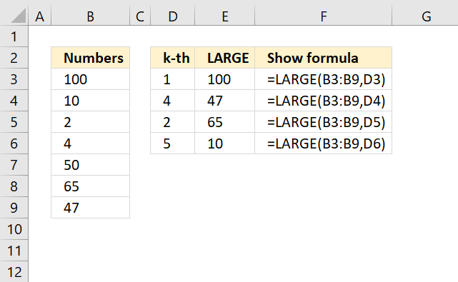
3. Example 1

The example demonstrated in cell E3 extracts the third-largest number in cell range B3:B9. Cell range B3:B9 contains random positive integers between 2 and 100.
Formula in cell C3:
The formula in cell C3 extracts the third largest number in B3:B9 which is 50. The largest is 100, the second largest is 65.
LARGE(array, k)
array - B3:B9
k - 3
LARGE(B3:B9, 3)
becomes
LARGE({100; 10; 2; 4; 50; 65; 47}, 3)
and returns 50. 50 is the third-largest number in B3:B9. Only 100 and 65 are larger.
4. Example 2 - based on a condition

The formula in cell F3 extracts the second largest number in cell range C3:C9 if the corresponding value on the same row in cell range B3:B9 is equal to the condition specified in cell E3.
Cell range B2:C9 contains the following values, cell E3 contains the condition which is "Apple" and cell F3 contains the formula.
| Item | Numbers |
| Apple | 100 |
| Orange | 10 |
| Apple | 2 |
| Orange | 4 |
| Apple | 50 |
| Banana | 65 |
| Apple | 47 |
Formula in cell F3:
The formula returns 50 which is the second highest number based on the specified condition "Apple". "Apple" is found in cells B3, B5, B7, and B9. The corresponding values in the same rows in column C are 100, 2, 50, and 47. The second largest number in this data set is 50.
4.1 Explaining formula
The Evaluate Formula tool is located on the Formulas tab in the Ribbon. It is a useful feature that allows you to step through and evaluate complex formulas to understand how the calculation is being performed and identify any errors or issues. The following steps shows these detailed evaluations for the formula above.
Step 1 - Logical test
The equal sign compares values in an Excel formula, the result is a boolean value TRUE or FALSE.
E3=B3:B9
becomes
"Apple"={"Apple"; "Orange"; "Apple"; "Orange"; "Apple"; "Orange"; "Apple"}
and returns
{TRUE; FALSE; TRUE; FALSE; TRUE; FALSE; TRUE}
Step 2 - Filter values based on logical test
The FILTER function extract values/rows based on a condition or criteria.
FILTER(array, include, [if_empty])
FILTER(C3:C9,E3=B3:B9)
becomes
FILTER(C3:C9,{TRUE; FALSE; TRUE; FALSE; TRUE; FALSE; TRUE})
becomes
FILTER({100; 10; 2; 4; 50; 65; 47},{TRUE; FALSE; TRUE; FALSE; TRUE; FALSE; TRUE})
and returns
{100; 2; 50; 47}
Step 3 - Calculate the second largest value
LARGE(FILTER(C3:C9,E3=B3:B9),2)
becomes
LARGE({100; 2; 50; 47},2)
and returns 50.
5. Example 3 - based on criteria

The formula in cell E3 extracts the second largest number in cell range C6:C12 if two conditions are met, the first condition is specified in cell B3 and the second in cell C3.
Note, the second condition is if a number is smaller than 60. Cell range B5:C12 contains data table with the following values:
| Item | Numbers |
| Apple | 100 |
| Orange | 10 |
| Apple | 2 |
| Orange | 4 |
| Apple | 50 |
| Banana | 65 |
| Apple | 47 |
Formula in cell E3:
The formula filters numbers if the corresponding value on the same row matches the condition specified in cell B3 which is "Apple" and if the number is smaller than 60 which is specified in cell C3.
The smaller than character is appended to the condition in the COUNTIFS function in the second argument pair:">"&C6:C12 The ampersand character lets you concatenate cell values with hardcoded values. The hardcoded values in this example is ">".
The valid numbers are 2, 50, and 47. The second largest number in this data set is 47 which matches the number in cell E3.
5.1 Explaining formula
Step 1 - Check criteria
The COUNTIFS function calculates the number of cells across multiple ranges that equals all given conditions.
COUNTIFS(criteria_range1, criteria1, [criteria_range2, criteria2]…)
Note the less than character in the last argument.
COUNTIFS(B3, B6:B12, C3, ">"&C6:C12)
returns
{0; 0; 1; 0; 1; 0; 1}.
Rows 8, 10 and 12 meet both conditions, see the image above.
Step 2 - Filter list
The FILTER function extract values/rows based on a condition or criteria.
FILTER(array, include, [if_empty])
FILTER(C6:C12, COUNTIFS(B3, B6:B12, C3, ">"&C6:C12))
becomes
FILTER(C6:C12, {0; 0; 1; 0; 1; 0; 1})
becomes
FILTER({100; 10; 2 ;4; 50; 65; 47}, {0; 0; 1; 0; 1; 0; 1})
and returns {2; 50; 47}.
Step 3 - Calculate the second largest value
LARGE(FILTER(C6:C12, COUNTIFS(B3, B6:B12, C3, ">"&C6:C12)), 2)
becomes
LARGE({2; 50; 47}, 2)
and returns 47.
6. Example 4 - based on a list

The formula in cell F3, in the image above, extracts the second largest number in cell range C3:C9 if the value on the same row in B3:B9 meets any of the conditions specified in cells E3 and E4.
In other words, OR logic applied to a single column meaning if "Apple" or "Banana" matches the value in cell B3:B9 then the corresponding number in cell C3:C9 is valid.
| Item | Numbers |
| Apple | 100 |
| Orange | 10 |
| Apple | 2 |
| Orange | 4 |
| Apple | 50 |
| Banana | 65 |
| Apple | 47 |
Formula in cell F3:
"Apple" or "Banana" are found in cells B3, B5, B7, B8 and B9. The corresponding numbers in cell C3:C9 are 100, 2, 50, 65 and 47. The second largest number in this data set is 65 which is the same value the formula returns in cell F3.
6.1 Explaining formula
Step 1 - Compare the list to items
The COUNTIF function counts the number of cells that meets a condition.
COUNTIF(range, criteria)
COUNTIF(E3:E4, B3:B9)
becomes
COUNTIF({"Apple"; "Banana"},{"Apple"; "Orange"; "Apple"; "Orange"; "Apple"; "Banana"; "Apple"})
and returns
{1; 0; 1; 0; 1; 1; 1}
Step 2 - Filter values based on logical test
The FILTER function extract values/rows based on a condition or criteria.
FILTER(array, include, [if_empty])
FILTER(C3:C9,COUNTIF(E3:E4, B3:B9))
becomes
FILTER(C3:C9,{1; 0; 1; 0; 1; 1; 1})
becomes
FILTER({100; 10; 2; 4; 50; 65; 47}, {1; 0; 1; 0; 1; 1; 1})
and returns
{100; 2; 50; 65, 47}.
Step 3 - Calculate the second largest value
LARGE(FILTER(C3:C9,E3=B3:B9),2)
becomes
LARGE({100; 2; 50; 65, 47},2)
and returns 65.
7. Example 5 - multiple source ranges

The formula in cell B3 extracts the second largest number from three different nonadjacent cell ranges: B7:B13, D7:D13, and F7:F13. They are in this example located on the same worksheet. The formula works fine even if they are on different worksheets. Here is the non-adjacent data:
| Numbers | Numbers | Numbers | ||
| 7 | 73 | 85 | ||
| 46 | 13 | 11 | ||
| 82 | 93 | 97 | ||
| 43 | 66 | 61 | ||
| 25 | 13 | 4 | ||
| 10 | 65 | 45 | ||
| 21 | 91 | 4 |
The arrays are joined using parentheses and commas between each cell reference.
Formula in cell B3:
The largest number in these cell ranges combines is 97, the second largest number is 93.
7.1 Explaining formula
The Evaluate Formula tool is located on the Formulas tab in the Ribbon. It is a useful feature that allows you to step through and evaluate complex formulas to understand how the calculation is being performed and identify any errors or issues. The following steps shows these detailed evaluations for the formula above.
Step 1 - Join cell ranges
The parentheses and commas let you join cell ranges in the LARGE function, this doesn't work in every function. However, the LARGE and SMALL function works.
(B7:B13,D7:D13,F7:F13)
becomes
({7; 46; 82; 43; 25; 10; 21},{73; 13; 93; 66; 13; 65; 91},{85; 11; 97; 61; 4; 45; 4})
and returns
{7,73,85; 46,13,11; 82,93,97; 43,66,61; 25,13,4; 10,65,45; 21,91,4}.
Step2 - Second largest value in the array
LARGE((B7:B13,D7:D13,F7:F13),2)
becomes
LARGE({7,73,85; 46,13,11; 82,93,97; 43,66,61; 25,13,4; 10,65,45; 21,91,4},2)
and returns 93. Only 97 is larger.
8. Example 6 - based on a text string

The formula in cell B6 splits the string specified in cell B3 into an array, then extracts the second largest number in the array.
The string is: "73,1,57,56,41,23,48,77,79,29", the TEXTSPLIT function splits the string using the specified delimiting character which in this case is a comma.
Excel sees the values in the array as text strings which makes it impossible for the LARGE function to handle. However, they are easy to convert, simply multiply by 1 and the result is a number.
Formula in cell B6:
The second largest number in "73,1,57,56,41,23,48,77,79,29" is 77. The largest number is 79.
8.1 Explaining formula
The Evaluate Formula tool is located on the Formulas tab in the Ribbon. It is a useful feature that allows you to step through and evaluate complex formulas to understand how the calculation is being performed and identify any errors or issues. The following steps shows these detailed evaluations for the formula above.
Step 1 - Split string
The TEXTSPLIT function lets you split a string into an array across columns and rows based on delimiting characters.
TEXTSPLIT(Input_Text, col_delimiter, [row_delimiter], [Ignore_Empty])
TEXTSPLIT(B3,",")
becomes
TEXTSPLIT("73,1,57,56,41,23,48,77,79,29",",")
and returns
{"73", "1", "57", "56", "41", "23", "48", "77", "79", "29"}.
Step 2 - Convert to numbers
The asterisk lets you multiply values in an Excel formula, it also lets you convert "text" numbers to regular numbers. The numbers in the array above have double quotes, these will be removed.
TEXTSPLIT(B3,",")*1
becomes
{"73", "1", "57", "56", "41", "23", "48", "77", "79", "29"}*1
and returns
{73, 1, 57, 56, 41, 23, 48, 77, 79, 29}.
Step 3 - Extract the second largest number in the array
LARGE(TEXTSPLIT(B3,",")*1,2)
becomes
LARGE({"73", "1", "57", "56", "41", "23", "48", "77", "79", "29"}, 2)
and returns 77. Only 79 is larger.
9. Example 7 - calculate an average of the three largest numbers

The formula in cell E3 extracts the three largest numbers in cell range B3:B9, then calculates an average based on these three numbers.
Excel is capable of doing multiple calculations in one cell and this is one example of that. This requires users with earlier Excel versions than Excel 365 to enter this formula as an array formula.
The second argument in the LARGE function is k, in this example we want to calculate the 3rd, 2nd, and the largest numbers which is possible if we use curly brackets: {1;2;3}
| Numbers |
| 100 |
| 10 |
| 2 |
| 4 |
| 50 |
| 66 |
| 47 |
The three largest numbers are 100, 66, and 50.
Formula in cell range E3:
To calculate the average, add up all the values or numbers in the data set. Count how many values or numbers there are in total in the data set. This is the number of data points. Divide the sum from by the number of data points. The result is the average.
100 + 66 + 50 = 216
216/3 = 72
9.1 Explaining formula
Step 1 - Extract the three largest numbers
The LARGE function allows you to extract multiple values if you use an array of numbers in the second argument.
LARGE(B3:B9,{1;2;3})
becomes
LARGE({100; 10; 2; 4; 50; 66; 47},{1; 2; 3})
and returns
{100; 66; 50}.
Step 2 - Calculate an average
The AVERAGE function calculates the average of numbers in a cell range or array.
AVERAGE(number1, [number2], ...)
AVERAGE(LARGE(B3:B9,{1; 2; 3}))
becomes
AVERAGE({100; 66; 50})
and returns 72. 100 + 66 + 50 = 216. 216/3 equals 72.
10. How to extract the k-th largest number in a 3D range

This example shows how to extract the k-th largest number in multiple worksheets. The data must be in the same cell range throughout all worksheets. For example, the image above demonstrates two cell ranges B3:B9 in worksheets '3D range' and '3D range (2)'.
Here is how to enter the LARGE function using 3D ranges:
- Doublepress with left mouse button on a cell.
- Type =LARGE(
- Press and hold SHIFT key.
- Select the remaining worksheets, in this case '3D range (2)' with the mouse.
- Select cell range B3:B9 with the mouse.
- Type the ending parentheses.
- Press Enter.
The formula looks like this;
Section 7 demonstrates how to get the k-th largest value from multiple cell ranges, this works fine with multiple worksheets as well and they don't need to be located on the same cell range. This can however be tedious to enter if many cell ranges are used.
11. Find smallest and largest unique number
![]()
This section explains how to calculate the largest and smallest number based on a condition which is if the number is unique. Unique meaning it exists only once in a column, numbers that have duplicates are not calculated.
I will also demonstrate how to calculate the k-th smallest or largest value based on the same condition using an array formula.
The image above shows a formula in cell D11, it extracts the largest unique number from column A. Cell D12 contains a formula that extracts the 100th largest unique number from column A.
What you will learn
- Build formulas that extract the min and max number if the number itself is unique.
- Identify unique numbers in a column.
- Create a formula that returns the k-th largest and smallest number if unique
Array formula in cell D11:
To enter an array formula press and hold CTRL + SHIFT simultaneously, then press Enter once. Release all keys.
The formula bar now shows the formula enclosed with curly brackets telling you that you entered the formula successfully. Don't enter the curly brackets yourself.
You will find an explanation of this formula below.
Array formula in cell D12:
This array formula in D12 returns the 100th largest unique number from column A.
Formula in cell D15:
This formula in D15 returns the largest number from column A, note it will also return a number that has a duplicate.
Formula in cell D16:
This formula in D16 returns the smallest number from column A, note it will also return a number that has a duplicate.
Array formula in cell G11:
This array formula in G11 is dynamic meaning it returns a different value in each cell, simply copy cell G11 and paste it to cells below. The ROW function utilizes a relative cell reference that changes when the formula is copied.
Explaining array formula in cell D11
Step 1 - Count the number of cells within a range that meet a given condition
The COUNTIF function counts cells that equals a specific value, the formula performs multiple calculations if we use multiple values and enter the formula as an array formula.
Note, we are using the same values in the first argument as in the second argument. The COUNTIF function returns a number larger than 1 if a value has a duplicate. COUNTIF(range, criteria)
COUNTIF(Table1[Value],Table1[Value])
returns
{1; 1; 1; 0; 1; 1; 1; 1; 1; ...}.
Step 2 - Check if value in array is a duplicate
The less than and larger than characters allow you to create a logical expression that returns either TRUE or FALSE.
COUNTIF(Table1[Value],Table1[Value])<> 1
becomes
{1; 1; 1; 0; 1; 1; 1; 1; 1; ...}<> 1
and returns
{FALSE; FALSE; FALSE; TRUE; FALSE; FALSE; FALSE; FALSE; FALSE; ...}.
Step 3 - Check if table value is a blank
We also need to figure out how to ignore blanks in column A, the equal sign lets you compare each value with nothing. It returns TRUE if a cell is blank.
(Table1[Value]="")
returns
{FALSE; FALSE; FALSE; TRUE; FALSE; FALSE; FALSE; FALSE; FALSE; ...}.
Step 4 - Return table value if conditions are met
The IF function lets your perform different actions based on a logical expression, in this case we want the formula to return "" (nothing) if TRUE and return the number itself if false.
IF((COUNTIF(Table1[Value],Table1[Value])< > 1)+(Table1[Value]=""),"",Table1[Value])
becomes
IF({FALSE; FALSE; FALSE; TRUE; FALSE; FALSE; FALSE; FALSE; FALSE; ...}, "", {72; 373; 230; 0; 311; 424; 460; 418; 665})
and returns
{72; 373; 230; ""; 311; 424; 460; 418; 665; ...}.
Step 5 - Return max value
The MAX function simply returns the largest number in the array or cell range.
MAX(IF((COUNTIF(Table1[Value],Table1[Value])< > 1)+(Table1[Value]=""),"",Table1[Value]))
becomes
=MAX({72; 373; 230; ""; 311; 424; 460; 418; 665; ...})
and returns 694 in cell D11.
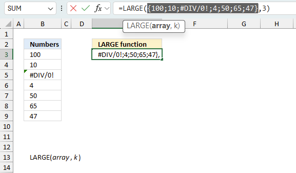
12. Function not working
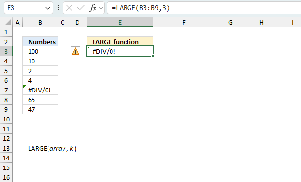
The LARGE function returns
- #VALUE! error if you use a non-numeric input value in the second argument k.
- #NUM! error if argument k is larger than the number of items in argument array.
- #NAME? error if you misspell the function name.
- propagates errors, meaning that if the input contains an error (e.g., #VALUE!, #REF!), the function will return the same error.
12.1 Troubleshooting the error value
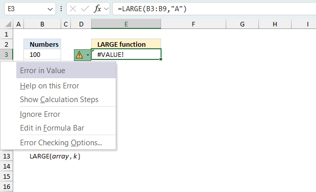
When you encounter an error value in a cell a warning symbol appears, displayed in the image above. Press with mouse on it to see a pop-up menu that lets you get more information about the error.
- The first line describes the error if you press with left mouse button on it.
- The second line opens a pane that explains the error in greater detail.
- The third line takes you to the "Evaluate Formula" tool, a dialog box appears allowing you to examine the formula in greater detail.
- This line lets you ignore the error value meaning the warning icon disappears, however, the error is still in the cell.
- The fifth line lets you edit the formula in the Formula bar.
- The sixth line opens the Excel settings so you can adjust the Error Checking Options.
Here are a few of the most common Excel errors you may encounter.
#NULL error - This error occurs most often if you by mistake use a space character in a formula where it shouldn't be. Excel interprets a space character as an intersection operator. If the ranges don't intersect an #NULL error is returned. The #NULL! error occurs when a formula attempts to calculate the intersection of two ranges that do not actually intersect. This can happen when the wrong range operator is used in the formula, or when the intersection operator (represented by a space character) is used between two ranges that do not overlap. To fix this error double check that the ranges referenced in the formula that use the intersection operator actually have cells in common.
#SPILL error - The #SPILL! error occurs only in version Excel 365 and is caused by a dynamic array being to large, meaning there are cells below and/or to the right that are not empty. This prevents the dynamic array formula expanding into new empty cells.
#DIV/0 error - This error happens if you try to divide a number by 0 (zero) or a value that equates to zero which is not possible mathematically.
#VALUE error - The #VALUE error occurs when a formula has a value that is of the wrong data type. Such as text where a number is expected or when dates are evaluated as text.
#REF error - The #REF error happens when a cell reference is invalid. This can happen if a cell is deleted that is referenced by a formula.
#NAME error - The #NAME error happens if you misspelled a function or a named range.
#NUM error - The #NUM error shows up when you try to use invalid numeric values in formulas, like square root of a negative number.
#N/A error - The #N/A error happens when a value is not available for a formula or found in a given cell range, for example in the VLOOKUP or MATCH functions.
#GETTING_DATA error - The #GETTING_DATA error shows while external sources are loading, this can indicate a delay in fetching the data or that the external source is unavailable right now.
12.2 The formula returns an unexpected value
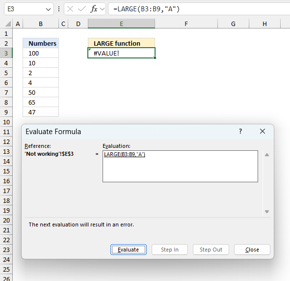
To understand why a formula returns an unexpected value we need to examine the calculations steps in detail. Luckily, Excel has a tool that is really handy in these situations. Here is how to troubleshoot a formula:
- Select the cell containing the formula you want to examine in detail.
- Go to tab “Formulas” on the ribbon.
- Press with left mouse button on "Evaluate Formula" button. A dialog box appears.
The formula appears in a white field inside the dialog box. Underlined expressions are calculations being processed in the next step. The italicized expression is the most recent result. The buttons at the bottom of the dialog box allows you to evaluate the formula in smaller calculations which you control. - Press with left mouse button on the "Evaluate" button located at the bottom of the dialog box to process the underlined expression.
- Repeat pressing the "Evaluate" button until you have seen all calculations step by step. This allows you to examine the formula in greater detail and hopefully find the culprit.
- Press "Close" button to dismiss the dialog box.
There is also another way to debug formulas using the function key F9. F9 is especially useful if you have a feeling that a specific part of the formula is the issue, this makes it faster than the "Evaluate Formula" tool since you don't need to go through all calculations to find the issue..
- Enter Edit mode: Double-press with left mouse button on the cell or press F2 to enter Edit mode for the formula.
- Select part of the formula: Highlight the specific part of the formula you want to evaluate. You can select and evaluate any part of the formula that could work as a standalone formula.
- Press F9: This will calculate and display the result of just that selected portion.
- Evaluate step-by-step: You can select and evaluate different parts of the formula to see intermediate results.
- Check for errors: This allows you to pinpoint which part of a complex formula may be causing an error.
The image above shows cell reference B3:B9 converted to hard-coded value using the F9 key. The LARGE function requires non-error values which is not the case in this example. We have found what is wrong with the formula.
Tips!
- View actual values: Selecting a cell reference and pressing F9 will show the actual values in those cells.
- Exit safely: Press Esc to exit Edit mode without changing the formula. Don't press Enter, as that would replace the formula part with the calculated value.
- Full recalculation: Pressing F9 outside of Edit mode will recalculate all formulas in the workbook.
Remember to be careful not to accidentally overwrite parts of your formula when using F9. Always exit with Esc rather than Enter to preserve the original formula. However, if you make a mistake overwriting the formula it is not the end of the world. You can “undo” the action by pressing keyboard shortcut keys CTRL + z or pressing the “Undo” button
12.3 Other errors
Floating-point arithmetic may give inaccurate results in Excel - Article
Floating-point errors are usually very small, often beyond the 15th decimal place, and in most cases don't affect calculations significantly.
'LARGE' function examples
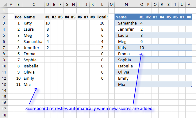
This article demonstrates a scoreboard, displayed to the left, that sorts contestants based on total scores and refreshes instantly each […]
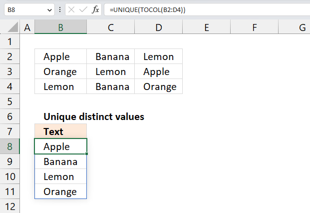
This article demonstrates ways to list unique distinct values in a cell range with multiple columns. The data is not […]
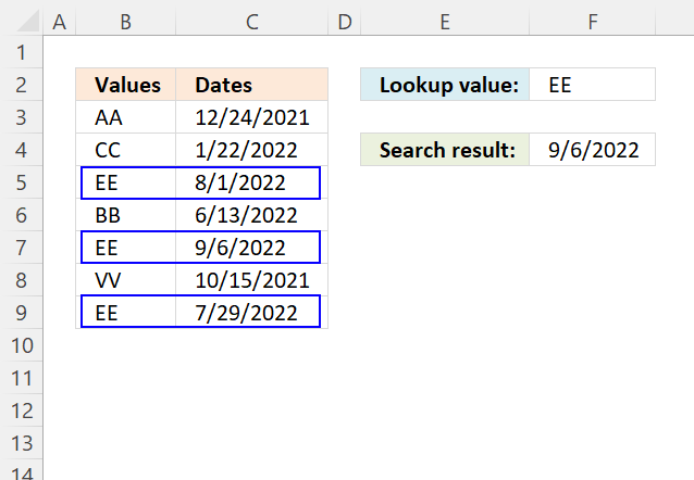
This article demonstrates how to return the latest date based on a condition using formulas or a Pivot Table. The […]
Functions in 'Statistical' category
The LARGE function function is one of 73 functions in the 'Statistical' category.
How to comment
How to add a formula to your comment
<code>Insert your formula here.</code>
Convert less than and larger than signs
Use html character entities instead of less than and larger than signs.
< becomes < and > becomes >
How to add VBA code to your comment
[vb 1="vbnet" language=","]
Put your VBA code here.
[/vb]
How to add a picture to your comment:
Upload picture to postimage.org or imgur
Paste image link to your comment.
Contact Oscar
You can contact me through this contact form