How to use the MODE.SNGL function

What is the MODE.SNGL function?

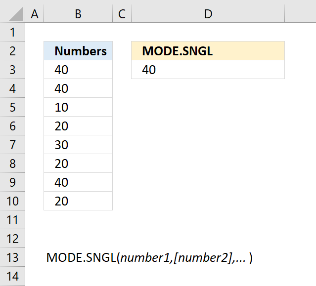
The MODE.SNGL function calculates the most frequent number in an array or cell range.

It returns only one value even if there are two or more equally frequent values.

1. Introduction

Can the MODE.SNGL function extract multiple mode values?

No, use the MODE.MULT function to extract multiple mode values if they are equally frequent.

Can the MODE.SNGL function extract the most common text value?

No, text, boolean values, and empty cells are ignored. There is a workaround, see section 5 below.

How to test if a distribution has multiple modes?

2. Syntax

MODE.SNGL(number1,[number2],...)

number1	Required. A number or cell reference for which you want to calculate the MODE.SNGL for.
[number2]	Optional. Up to 254 additional arguments.

3. Example

The image above demonstrates the MODE.SNGL function. It extracts the most frequent number from cell range B3:B10. That is 40 in this example, it exists three times and is the most repeated number.

Formula in cell D3:

This function is entered as a regular function, it returns only one value.

How to create a frequency table based on numerical values
How to create a frequency table based on text values

Back to top

4. Function not working

MODE.SNGL function returns #N/A error value if the source data set contains no duplicates.

It also returns an error if the source data contains an error, you can handle this by using the IFERROR function and convert errors to text values that the function then ignores. The data in cell range B3:B10, displayed in the image above, is:

Numbers
40
40
10
#DIV/0!
30
20
40
20

Here is an example that removes error values and converts them to blank values "".

This formula ignores the error value and returns 40 which is the most frequent number in B3:B10.

4.1 Troubleshooting the error value

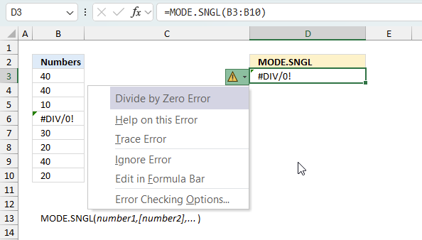
When you encounter an error value in a cell a warning symbol appears, displayed in the image above. Press with mouse on it to see a pop-up menu that lets you get more information about the error.

1. The first line describes the error if you press with left mouse button on it.
2. The second line opens a pane that explains the error in greater detail.
3. The third line takes you to the "Evaluate Formula" tool, a dialog box appears allowing you to examine the formula in greater detail.
4. This line lets you ignore the error value meaning the warning icon disappears, however, the error is still in the cell.
5. The fifth line lets you edit the formula in the Formula bar.
6. The sixth line opens the Excel settings so you can adjust the Error Checking Options.

Here are a few of the most common Excel errors you may encounter.

#NULL error - This error occurs most often if you by mistake use a space character in a formula where it shouldn't be. Excel interprets a space character as an intersection operator. If the ranges don't intersect an #NULL error is returned. The #NULL! error occurs when a formula attempts to calculate the intersection of two ranges that do not actually intersect. This can happen when the wrong range operator is used in the formula, or when the intersection operator (represented by a space character) is used between two ranges that do not overlap. To fix this error double check that the ranges referenced in the formula that use the intersection operator actually have cells in common.

#SPILL error - The #SPILL! error occurs only in version Excel 365 and is caused by a dynamic array being to large, meaning there are cells below and/or to the right that are not empty. This prevents the dynamic array formula expanding into new empty cells.

#DIV/0 error - This error happens if you try to divide a number by 0 (zero) or a value that equates to zero which is not possible mathematically.

#VALUE error - The #VALUE error occurs when a formula has a value that is of the wrong data type. Such as text where a number is expected or when dates are evaluated as text.

#REF error - The #REF error happens when a cell reference is invalid. This can happen if a cell is deleted that is referenced by a formula.

#NAME error - The #NAME error happens if you misspelled a function or a named range.

#NUM error - The #NUM error shows up when you try to use invalid numeric values in formulas, like square root of a negative number.

#N/A error - The #N/A error happens when a value is not available for a formula or found in a given cell range, for example in the VLOOKUP or MATCH functions.

#GETTING_DATA error - The #GETTING_DATA error shows while external sources are loading, this can indicate a delay in fetching the data or that the external source is unavailable right now.

4.2 The formula returns an unexpected value

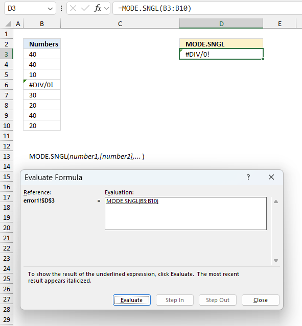
To understand why a formula returns an unexpected value we need to examine the calculations steps in detail. Luckily, Excel has a tool that is really handy in these situations. Here is how to troubleshoot a formula:

1. Select the cell containing the formula you want to examine in detail.
2. Go to tab “Formulas” on the ribbon.
3. Press with left mouse button on "Evaluate Formula" button. A dialog box appears.
   The formula appears in a white field inside the dialog box. Underlined expressions are calculations being processed in the next step. The italicized expression is the most recent result. The buttons at the bottom of the dialog box allows you to evaluate the formula in smaller calculations which you control.
4. Press with left mouse button on the "Evaluate" button located at the bottom of the dialog box to process the underlined expression.
5. Repeat pressing the "Evaluate" button until you have seen all calculations step by step. This allows you to examine the formula in greater detail and hopefully find the culprit.
6. Press "Close" button to dismiss the dialog box.

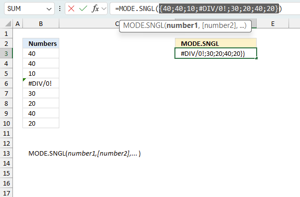
There is also another way to debug formulas using the function key F9. F9 is especially useful if you have a feeling that a specific part of the formula is the issue, this makes it faster than the "Evaluate Formula" tool since you don't need to go through all calculations to find the issue.

1. Enter Edit mode: Double-press with left mouse button on the cell or press F2 to enter Edit mode for the formula.
2. Select part of the formula: Highlight the specific part of the formula you want to evaluate. You can select and evaluate any part of the formula that could work as a standalone formula.
3. Press F9: This will calculate and display the result of just that selected portion.
4. Evaluate step-by-step: You can select and evaluate different parts of the formula to see intermediate results.
5. Check for errors: This allows you to pinpoint which part of a complex formula may be causing an error.

The image above shows cell reference B3:B10 converted to hard-coded value using the F9 key. The MODE.SNGL function requires non-error values which is not the case in this example. We have found what is wrong with the formula.

Tips!

• View actual values: Selecting a cell reference and pressing F9 will show the actual values in those cells.
• Exit safely: Press Esc to exit Edit mode without changing the formula. Don't press Enter, as that would replace the formula part with the calculated value.
• Full recalculation: Pressing F9 outside of Edit mode will recalculate all formulas in the workbook.

Remember to be careful not to accidentally overwrite parts of your formula when using F9. Always exit with Esc rather than Enter to preserve the original formula. However, if you make a mistake overwriting the formula it is not the end of the world. You can “undo” the action by pressing keyboard shortcut keys CTRL + z or pressing the “Undo” button

4.3 Other errors

Floating-point arithmetic may give inaccurate results in Excel - Article

Floating-point errors are usually very small, often beyond the 15th decimal place, and in most cases don't affect calculations significantly.

Back to top

5. Extract the most frequent text value - MODE.SNGL function

The MODE.SNGL calculates the most frequent number, it ignores text and boolean values. This example demonstrates a formula that extracts the most frequent text value in a given cell range.

The formula in cell D3 extracts the most frequent text value from cell range B3:B16. It will only return a single value even if there are multiple mode values that are equally frequent.
How to test if a distribution has multiple modes?

Cell range B3:B16 contains student grades from A to E, cells D3 and D4 contain grade "D" and "C". They are equally frequent in B3:B16.

Excel 365 formula in cell D3:

If you need to extract multiple mode text values, read this:
Extract the most frequent text values

Explaining formula

Step 1 - Find relative position in the array

The MATCH function returns the relative position of an item in an array that matches a specified value in a specific order.

Function syntax: MATCH(lookup_value, lookup_array, [match_type])

MATCH(B3:B16,B3:B16,0)

becomes

MATCH({"D";"E";"C";"D";"A";"E";"D";"B";"D";"C";"B";"D";"C";"B"},{"D";"E";"C";"D";"A";"E";"D";"B";"D";"C";"B";"D";"C";"B"},0)

and returns

{1;2;3;1;5;2;1;8;1;3;8;1;3;8}.

Step 2 - Calculate the mode

The MODE.SNGL function calculates the most frequent value in an array or range of data.

Function syntax: MODE.SNGL(number1,[number2],...)

MODE.SNGL(MATCH(B3:B16,B3:B16,0))

becomes

MODE.SNGL({1;2;3;1;5;2;1;8;1;3;8;1;3;8})

and returns 1.

Step 3 - Find the position of the mode numbers in the array

The MATCH function returns the relative position of an item in an array that matches a specified value in a specific order.

Function syntax: MATCH(lookup_value, lookup_array, [match_type])

MATCH(MODE.SNGL(MATCH(B3:B16,B3:B16,0)),MATCH(B3:B16,B3:B16,0),0)

becomes

MATCH(1,{1;2;3;1;5;2;1;8;1;3;8;1;3;8},0)

and returns 1.

Step 4 - Get text values from the corresponding positions

The INDEX function returns a value or reference from a cell range or array, you specify which value based on a row and column number.

Function syntax: INDEX(array, [row_num], [column_num])

INDEX(B3:B16,MATCH(MODE.SNGL(MATCH(B3:B16,B3:B16,0)),MATCH(B3:B16,B3:B16,0),0))

becomes

INDEX(B3:B16,1)

and returns "D".

Step 5 - Shorten formula

The LET function lets you name intermediate calculation results which can shorten formulas considerably and improve performance.

Function syntax: LET(name1, name_value1, calculation_or_name2, [name_value2, calculation_or_name3...])

INDEX(B3:B16,MATCH(MODE.SNGL(MATCH(B3:B16,B3:B16,0)),MATCH(B3:B16,B3:B16,0),0))

MATCH(B3:B16,B3:B16,0) is repeated twice.

x - MATCH(B3:B16,B3:B16,0)

B3:B16 is repeated three times.

y - B3:B16

LET(y,B3:B16,x,MATCH(y,y,0),INDEX(y,MATCH(MODE.SNGL(x),x,0)))

Back to top

6. How to create a frequency table based on text values

What is a frequency table?

A frequency table in statistics is a method of summarizing a data set by showing how often each value or category is repeated. A frequency table usually has two or more columns: one for the values or categories of the variable, and one for the frequencies. A frequency table may also show relative frequency and cumulative frequency.

I demonstrated here: How to create a frequency table based on numerical values, this example shows a formula that creates a frequency table based on text values.

You need Excel 365 to use the following formula, it is entered as a regular formula, however, it spills values below and to the right as far as needed.

Excel 365 formula in cell D4:

This formula creates a frequency table and sorts the output by frequency from large to small. The image above shows that grade "D" is the most common and then "C","B", "E", and lastly "A".

The formula above will not work if your data is arranged across multiple columns, read the following article if that is the case:
Extract a unique distinct list across multiple columns and rows sorted based on frequency

Explaining formula in cell D4

Step 1 - Find relative position

The MATCH function returns the relative position of an item in an array that matches a specified value in a specific order.

Function syntax: MATCH(lookup_value, lookup_array, [match_type])

MATCH(B3:B16,B3:B16,0)

becomes

MATCH({"D";"E";"C";"D";"A";"E";"D";"B";"D";"C";"B";"D";"C";"B"},{"D";"E";"C";"D";"A";"E";"D";"B";"D";"C";"B";"D";"C";"B"},0)

and returns

{1;2;3;1;5;2;1;8;1;3;8;1;3;8}

Step 2 - Extract unique distinct numerical values

The UNIQUE function returns a unique or unique distinct list.

Function syntax: UNIQUE(array,[by_col],[exactly_once])

UNIQUE(MATCH(B3:B16,B3:B16,0))

becomes

UNIQUE({1;2;3;1;5;2;1;8;1;3;8;1;3;8})

and returns

{1;2;3;5;8}

Step 3 - Calculate frequency

The FREQUENCY function calculates how often values occur within a range of values and then returns a vertical array of numbers.

Function syntax: FREQUENCY(data_array, bins_array)

FREQUENCY(MATCH(B3:B16,B3:B16,0),UNIQUE(MATCH(B3:B16,B3:B16,0)))

becomes

FREQUENCY({1;2;3;1;5;2;1;8;1;3;8;1;3;8},{1;2;3;5;8})

and returns

{5;2;3;1;3;0}

Step 4 - Extract unique distinct text values

The UNIQUE function returns a unique or unique distinct list.

Function syntax: UNIQUE(array,[by_col],[exactly_once])

UNIQUE(B3:B16)

becomes

UNIQUE({"D";"E";"C";"D";"A";"E";"D";"B";"D";"C";"B";"D";"C";"B"})

and returns

{"D";"E";"C";"A";"B"}.

Step 5 - Stack arrays horizontally

The HSTACK function combines cell ranges or arrays. Joins data to the first blank cell to the right of a cell range or array (horizontal stacking)

Function syntax: HSTACK(array1,[array2],...)

HSTACK(UNIQUE(B3:B16),FREQUENCY(MATCH(B3:B16,B3:B16,0),UNIQUE(MATCH(B3:B16,B3:B16,0))))

becomes

HSTACK({"D";"E";"C";"A";"B"},{5;2;3;1;3;0})

and returns

{"D",5;"E",2;"C",3;"A",1;"B",3;#N/A,0}

Step 6 - Remove last row

The DROP function removes a given number of rows or columns from a 2D cell range or array.

Function syntax: DROP(array, rows, [columns])

DROP(HSTACK(UNIQUE(B3:B16),FREQUENCY(MATCH(B3:B16,B3:B16,0),UNIQUE(MATCH(B3:B16,B3:B16,0)))),-1)

becomes

DROP({"D",5;"E",2;"C",3;"A",1;"B",3;#N/A,0},-1)

and returns

{"D",5;"E",2;"C",3;"A",1;"B",3}.

Step 7 - Sort array by the frequency

The SORT function sorts values from a cell range or array

Function syntax: SORT(array,[sort_index],[sort_order],[by_col])

SORT(DROP(HSTACK(UNIQUE(B3:B16),FREQUENCY(MATCH(B3:B16,B3:B16,0),UNIQUE(MATCH(B3:B16,B3:B16,0)))),-1),2,-1)

becomes

SORT({"D",5;"E",2;"C",3;"A",1;"B",3})

and returns

{"D",5;"C",3;"B",3;"E",2;"A",1}.

Step 8 - Shorten formula

The LET function lets you name intermediate calculation results which can shorten formulas considerably and improve performance.

Function syntax: LET(name1, name_value1, calculation_or_name2, [name_value2, calculation_or_name3...])

SORT(DROP(HSTACK(UNIQUE(B3:B16),FREQUENCY(MATCH(B3:B16,B3:B16,0),UNIQUE(MATCH(B3:B16,B3:B16,0)))),-1),2,-1)

MATCH(B3:B16,B3:B16,0) is repeated twice.

x - MATCH(B3:B16,B3:B16,0)

B3:B16 is repeated three times.

y- B3:B16

LET(y,B3:B16,x,MATCH(y,y,0),SORT(DROP(HSTACK(UNIQUE(y),FREQUENCY(x,UNIQUE(x))),-1),2,-1))

Back to top

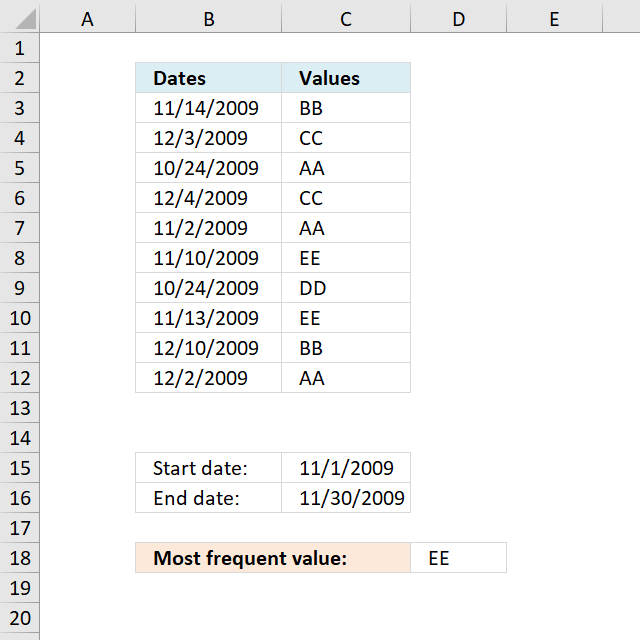
7. Most frequent value between two dates

Update! Oct 10th, 2024 - shorter formula

Array formula in D18:

Excel 365 users may skip these steps, you are not required to enter the formula as an array formula.

1. To enter an array formula, type the formula in a cell.
2. Press and hold CTRL + SHIFT simultaneously.
3. Press Enter once.
4. Release all keys.

The formula bar now shows the formula with a beginning and ending curly bracket telling you that you entered the formula successfully. Don't enter the curly brackets yourself.

Back to top

7.1 Explaining the formula in cell D18

Older formula:

=INDEX($C$3:$C$12, MATCH(MODE.SNGL(IF(($B$3:$B$12<=$C$16)*($B$3:$B$12>=$C$15), COUNTIF($C$3:$C$12, "<"&$C$3:$C$12), "")), COUNTIF($C$3:$C$12, "<"&$C$3:$C$12),0))

Step 1 - Calculate rank order if sorted

The COUNTIF function counts values based on a condition or criteria, the < less than sign makes the COUNTIF calculate a rank number if the list were sorted from A to Z.

COUNTIF($C$3:$C$12,"<"&$C$3:$C$12)

becomes

COUNTIF({"BB"; "CC"; "AA"; "CC"; "AA"; "EE"; "DD"; "EE"; "BB"; "AA"},"<"&{"BB"; "CC"; "AA"; "CC"; "AA"; "EE"; "DD"; "EE"; "BB"; "AA"})

becomes

COUNTIF({"BB"; "CC"; "AA"; "CC"; "AA"; "EE"; "DD"; "EE"; "BB"; "AA"}, {"<BB";"<CC";"<AA";"<CC";"<AA";"<EE";"<DD";"<EE";"<BB";"<AA"})

and returns

{3;5;0;5;0;8;7;8;3;0}.

Step 2 - Check which values are in range

The IF function returns the rank number number based on a logical expression. It returns boolean value TRUE if the value is in the date range. If boolean value is FALSE the IF function returns "" (nothing).

IF(($B$3:$B$12<=$C$16)*($B$3:$B$12>=$C$15),COUNTIF($C$3:$C$12,"<"&$C$3:$C$12),"")

becomes

IF({1;0;0;0;1;1;0;1;0;0},COUNTIF($C$3:$C$12,"<"&$C$3:$C$12),"")

becomes

IF({1;0;0;0;1;1;0;1;0;0}, {3; 5; 0; 5; 0; 8; 7; 8; 3; 0},"")

and returns

{3; ""; ""; ""; 0; 8; ""; 8; ""; ""}.

Step 3 - Calculate the most frequent number

The MODE.SNGL function returns the most frequent number in a cell range or array.

MODE.SNGL(IF(($B$3:$B$12<=$C$16)*($B$3:$B$12>=$C$15),COUNTIF($C$3:$C$12,"<"&$C$3:$C$12),""))

becomes

MODE.SNGL({3; ""; ""; ""; 0; 8; ""; 8; ""; ""})

and returns 8.

Step 4 - Find position of most frequent number in array

The MATCH function finds the relative position of a value in an array or cell range.

MATCH(MODE.SNGL(IF(($B$3:$B$12<=$C$16)*($B$3:$B$12>=$C$15), COUNTIF($C$3:$C$12, "<"&$C$3:$C$12), "")), COUNTIF($C$3:$C$12, "<"&$C$3:$C$12),0)

becomes

MATCH(8, COUNTIF($C$3:$C$12, "<"&$C$3:$C$12),0)

becomes

MATCH(8, {3; 5; 0; 5; 0; 8; 7; 8; 3; 0},0)

and returns 6.

Step 5 - Return value

The INDEX function returns a value based on row number (and column number if needed)

INDEX($C$3:$C$12, MATCH(MODE.SNGL(IF(($B$3:$B$12<=$C$16)*($B$3:$B$12>=$C$15), COUNTIF($C$3:$C$12, "<"&$C$3:$C$12), "")), COUNTIF($C$3:$C$12, "<"&$C$3:$C$12),0))

becomes

INDEX($C$3:$C$12, 6)

and returns "EE" in cell D18.

Back to top

Get Excel *.xlsx file

Most common value between two dates.xlsx

Back to top

8. Most frequent value between two dates - Autofilter

This example demonstrates how to identify the most repeated value in a filtered data set using the Autofilter feature and two formulas.

Excel 365 dynamic array formula in cell B15:

This Excel 365 formula can be used without the helper column in column D. It is also somewhat smaller than the older formula demonstrated below.

Formula in cell B15:

Formula in cell D3:

Copy cell D3 and paste to the cells below.

Back to top

8.1 Explaining formula in cell D3

Step 1 - Populate arguments

The SUBTOTAL function returns a subtotal from a list or database, you can choose from a variety of arguments that determine what you want the function to do.

Function syntax: SUBTOTAL(function_num, ref1, ...)

SUBTOTAL(function_num, ref1, ...)

becomes

SUBTOTAL(3,C3)

Step 2 - Evaluate SUBTOTAL function

SUBTOTAL(3,C3)

becomes

SUBTOTAL(3,"BB")

and returns 1.

Step 3 - Check if the value is equal to 1

The equal sign is a logical operator, it compares value to value. The result is a boolean value TRUE or FALSE.

SUBTOTAL(3, C3)=1

becomes

1=1

and returns

TRUE.

Back to top

8.2 Explaining formula in cell B15

Step 1 - Check which rows are visible

The equal sign is a logical operator, it compares value to value. The result is a boolean value TRUE or FALSE.

D3:D12=TRUE

{TRUE;0;0;0;TRUE;TRUE;0;0;TRUE;FALSE} = TRUE

and returns

{TRUE; FALSE; FALSE; FALSE; TRUE; TRUE; FALSE; FALSE; TRUE; FALSE}.

Step 2 - Convert text values to unique numbers

The COUNTIF function calculates the number of cells that is equal to a condition.

Function syntax: COUNTIF(range, criteria)

COUNTIF($C$3:$C$12, "<"&$C$3:$C$12)

becomes

COUNTIF({"BB"; "CC"; "AA"; "CC"; "AA"; "EE"; "AA"; "DD"; "EE"; "BB"}, "<"&{"BB"; "CC"; "AA"; "CC"; "AA"; "EE"; "AA"; "DD"; "EE"; "BB"})

and returns

{3; 5; 0; 5; 0; 8; 0; 7; 8; 3}.

Step 3 - Replace visible values with a unique number

The IF function returns one value if the logical test is TRUE and another value if the logical test is FALSE.

Function syntax: IF(logical_test, [value_if_true], [value_if_false])

IF(D3:D12=1, COUNTIF($C$3:$C$12, "<"&$C$3:$C$12), "")

becomes

IF(TRUE; FALSE; FALSE; FALSE; TRUE; TRUE; FALSE; FALSE; TRUE; FALSE}, {3; 5; 0; 5; 0; 8; 0; 7; 8; 3}, "")

and returns

{3; ""; ""; ""; 0; 8; ""; ""; 8; ""}

Step 4 - Find the most repeated number

The MODE.SNGL function calculates the most frequent value in an array or range of data.

Function syntax: MODE.SNGL(number1,[number2],...)

MODE.SNGL(IF(D3:D12=1, COUNTIF($C$3:$C$12, "<"&$C$3:$C$12), ""))

becomes

MODE.SNGL({3; ""; ""; ""; 0; 8; ""; ""; 8; ""})

and returns 8.

Step 5 - Find the relative position of the most repeated number

The MATCH function returns the relative position of an item in an array that matches a specified value in a specific order.

Function syntax: MATCH(lookup_value, lookup_array, [match_type])

MATCH(MODE.SNGL(IF(D3:D12=1, COUNTIF($C$3:$C$12, "<"&$C$3:$C$12), "")), COUNTIF($C$3:$C$12, "<"&$C$3:$C$12), 0)

becomes

MATCH(8, {3; 5; 0; 5; 0; 8; 0; 7; 8; 3}, 0)

and returns

6.

Step 6 - Get the corresponding value in $C$3:$C$12

The INDEX function returns a value or reference from a cell range or array, you specify which value based on a row and column number.

Function syntax: INDEX(array, [row_num], [column_num])

INDEX($C$3:$C$12, MATCH(MODE.SNGL(IF(D3:D12=1, COUNTIF($C$3:$C$12, "<"&$C$3:$C$12), "")), COUNTIF($C$3:$C$12, "<"&$C$3:$C$12), 0))

becomes

INDEX($C$3:$C$12, 6)

becomes

INDEX({"BB"; "CC"; "AA"; "CC"; "AA"; "EE"; "AA"; "DD"; "EE"; "BB"}, 6)

and returns

"EE".

Back to top

8.3 How to enable the Autofilter

How do I enable the autofilter for a given data set (shortcut keys)?

1. Select any cell in the data set.
2. Press and hold CTRL and Shift keys.
3. Press L once.
4. Release all keys.

How do I enable the autofilter for a given data set (button on the ribbon)?

1. Select any cell in the data set.
2. Go to tab "Data".
3. Press with left mouse button on the "Filter" button.

How do I know autofilter is enabled?

The column header names have a small button each containing an arrow, see the image above.

Back to top

8.4 Enter the formula in cell D3

Copy cell D3 and paste to the cells below.

Make sure the new column header has the autofilter arrow. If not, disable the autofilter and then enable it again.

Back to top

8.5 How to apply a condition to the Autofilter

1. Press with mouse on a button next to a column you want to filter.
   
2. A popup menu appears. Deselect all check boxes except "November".
   
3. Press with left mouse button on "OK" button.

Back to top

8.6 How to know if a data set is filtered - Autofilter?

There are two ways you can see if a data set is filtered, the first one is the button.

The button next to column header name "Date" has changed from an arrow to an icon that tells you the data is filtered.

The second one is the row color, filtered data has blue row numbers.

Back to top

8.7 How to clear a filter - Autofilter?

1. Press with mouse on the button next to the column header name you want to clear.
   
2. A popup menu appears. Press with left mouse button on "Clear Filter from "Dates"

Filter for that particular column is now removed.

Back to top

Useful links

I have more about the mode or modal in statistics written here:

• What is the mode or modal in statistics?
• Why calculate the most frequent value (mode or modal)?
• How can you interpret the mode in relation to the mean and median?
• What is the difference between the MODE.SNGL, MODE.MULT, and the MODE functions?

MODE.SNGL function - Microsoft
Mode: What It Is in Statistics and How to Calculate It
Mode (statistics) - wikipedia

Back to top

Back to top

 

'MODE.SNGL' function examples

The following article has a formula that contains the MODE.SNGL function.

Functions in 'Statistical' category

The MODE.SNGL function function is one of 73 functions in the 'Statistical' category.

Excel function categories

Excel categories

Comments (3)