How to use the SORTBY function

The SORTBY function allows you to sort values from a cell range or array based on a corresponding cell range or array. It sorts values by column but keeps rows.
It is located in the Lookup and reference category and is only available to Excel 365 subscribers.
What's on this page
- Syntax
- Arguments
- Example
- What is a spilled array formula?
- Function not working
- Does the function differentiate between upper and lower letters?
- How to sort two columns from A to Z
- How to sort from Z to A?
- How to sort from smallest to largest?
- How to sort from largest to smallest?
- How to sort by multiple columns?
- Sort by another column
- Sort by the first letter/digit?
- Sort by absolute value?
- Sort by the last word in a cell?
- Sort by the first name?
- Sort by the last name?
- Sort by custom list?
- Sort by month?
- Sort by word length
- Sort in random order
- Sort unique values in random order
- Sort by week number
- Sort by quarter
- Sort based on row count
- Sort numbers based on proximity to a given number
- Sort based on frequency row-wise
- Sort by multiple columns using an Excel Table
- Sort by multiple columns using the SORTBY function (Excel 365)
- Sort by multiple columns using formula (Previous Excel versions)
1. Syntax
SORTBY(array, by_array1, [sort_order1], [by_array2, sort_order2],…)
2. Arguments
| Argument | Text |
| array | Required. Cell range or array. |
| by_array1 | Required. A cell range or array. |
| [sort_order1] | Optional. Sort order for argument by_array1. 1 - Ascending order (A to Z or small to large) -1 - descending order (Z to A or large to small). 1 is the default value if the argument is not specified. |
| [by_array2] | Optional. The cell range or array. |
| [sort_order2] | Optional. Sort order for argument [by_array2]. 1 - Ascending order (A to Z or small to large) -1 - descending order (Z to A or large to small). 1 is the default value if the argument is not specified. |
3. Example
Formula in cell D3:
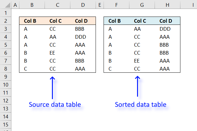
The formula demonstrated in the image above sorts the data in cell range B3:D8 by column B and then column C and lastly column D in ascending order, and returns the sorted array to cell F3. This is not possible using the SORT function, the SORTBY function is more advanced.
4. What is a spilled array formula?

Excel 365 automatically expands the output range based on the number of values in the array, this without requiring the user to enter the formula as an array formula.
This new behavior of Excel is called spilled array formula and is something only dynamic array formulas can do. Dynamic array formulas are only available to Excel 365 subscribers.
5. Function not working

If the needed cell range is populated by any other value a #SPILL! error is returned by the SORTBY function. You have two options:
- Remove value leaving the cell blank.
- Enter the dynamic formula in another cell that has empty adjacent cells.

If a cell returns #NAME! error you have either spelled the function name wrong or you use an incompatible Excel version.
The image above shows that I spelled the SORTBY function wrong in the formula bar, cell F3 displays #NAME! error.
Only Excel 365 subscription version supports the new dynamic array formula like the SORTBY function, older Excel versions like Excel 2019, 2016, 2013, 2010, 2007 and earlier versions do not support the SORTBY function.
Here is how to find out your Excel version: Get your Excel version
5.1 Troubleshooting the error value
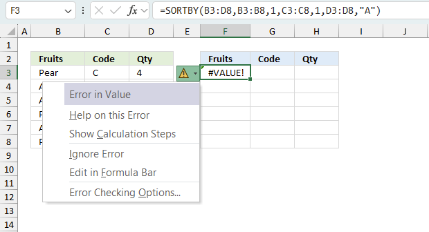
When you encounter an error value in a cell a warning symbol appears, displayed in the image above. Press with mouse on it to see a pop-up menu that lets you get more information about the error.
- The first line describes the error if you press with left mouse button on it.
- The second line opens a pane that explains the error in greater detail.
- The third line takes you to the "Evaluate Formula" tool, a dialog box appears allowing you to examine the formula in greater detail.
- This line lets you ignore the error value meaning the warning icon disappears, however, the error is still in the cell.
- The fifth line lets you edit the formula in the Formula bar.
- The sixth line opens the Excel settings so you can adjust the Error Checking Options.
Here are a few of the most common Excel errors you may encounter.
#NULL error - This error occurs most often if you by mistake use a space character in a formula where it shouldn't be. Excel interprets a space character as an intersection operator. If the ranges don't intersect an #NULL error is returned. The #NULL! error occurs when a formula attempts to calculate the intersection of two ranges that do not actually intersect. This can happen when the wrong range operator is used in the formula, or when the intersection operator (represented by a space character) is used between two ranges that do not overlap. To fix this error double check that the ranges referenced in the formula that use the intersection operator actually have cells in common.
#SPILL error - The #SPILL! error occurs only in version Excel 365 and is caused by a dynamic array being to large, meaning there are cells below and/or to the right that are not empty. This prevents the dynamic array formula expanding into new empty cells.
#DIV/0 error - This error happens if you try to divide a number by 0 (zero) or a value that equates to zero which is not possible mathematically.
#VALUE error - The #VALUE error occurs when a formula has a value that is of the wrong data type. Such as text where a number is expected or when dates are evaluated as text.
#REF error - The #REF error happens when a cell reference is invalid. This can happen if a cell is deleted that is referenced by a formula.
#NAME error - The #NAME error happens if you misspelled a function or a named range.
#NUM error - The #NUM error shows up when you try to use invalid numeric values in formulas, like square root of a negative number.
#N/A error - The #N/A error happens when a value is not available for a formula or found in a given cell range, for example in the VLOOKUP or MATCH functions.
#GETTING_DATA error - The #GETTING_DATA error shows while external sources are loading, this can indicate a delay in fetching the data or that the external source is unavailable right now.
5.2 The formula returns an unexpected value
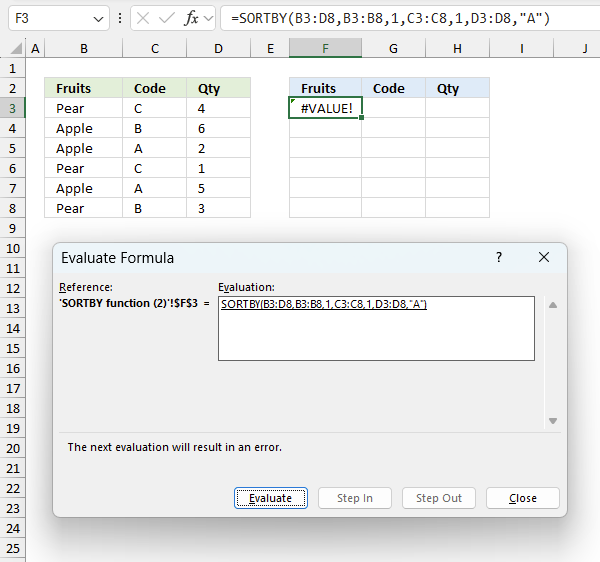
To understand why a formula returns an unexpected value we need to examine the calculations steps in detail. Luckily, Excel has a tool that is really handy in these situations. Here is how to troubleshoot a formula:
- Select the cell containing the formula you want to examine in detail.
- Go to tab “Formulas” on the ribbon.
- Press with left mouse button on "Evaluate Formula" button. A dialog box appears.
The formula appears in a white field inside the dialog box. Underlined expressions are calculations being processed in the next step. The italicized expression is the most recent result. The buttons at the bottom of the dialog box allows you to evaluate the formula in smaller calculations which you control. - Press with left mouse button on the "Evaluate" button located at the bottom of the dialog box to process the underlined expression.
- Repeat pressing the "Evaluate" button until you have seen all calculations step by step. This allows you to examine the formula in greater detail and hopefully find the culprit.
- Press "Close" button to dismiss the dialog box.
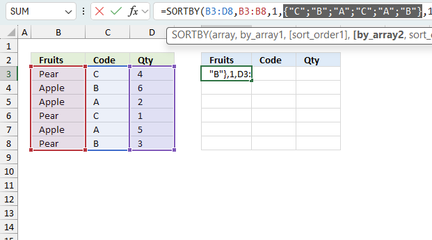
There is also another way to debug formulas using the function key F9. F9 is especially useful if you have a feeling that a specific part of the formula is the issue, this makes it faster than the "Evaluate Formula" tool since you don't need to go through all calculations to find the issue.
- Enter Edit mode: Double-press with left mouse button on the cell or press F2 to enter Edit mode for the formula.
- Select part of the formula: Highlight the specific part of the formula you want to evaluate. You can select and evaluate any part of the formula that could work as a standalone formula.
- Press F9: This will calculate and display the result of just that selected portion.
- Evaluate step-by-step: You can select and evaluate different parts of the formula to see intermediate results.
- Check for errors: This allows you to pinpoint which part of a complex formula may be causing an error.
The image above shows cell reference C3:C8 converted to hard-coded value using the F9 key. The SORTBY function requires numerical values between 0 (zero) and 1 which is not the case in this example. We have found what is wrong with the formula.
Tips!
- View actual values: Selecting a cell reference and pressing F9 will show the actual values in those cells.
- Exit safely: Press Esc to exit Edit mode without changing the formula. Don't press Enter, as that would replace the formula part with the calculated value.
- Full recalculation: Pressing F9 outside of Edit mode will recalculate all formulas in the workbook.
Remember to be careful not to accidentally overwrite parts of your formula when using F9. Always exit with Esc rather than Enter to preserve the original formula. However, if you make a mistake overwriting the formula it is not the end of the world. You can “undo” the action by pressing keyboard shortcut keys CTRL + z or pressing the “Undo” button
5.3 Other errors
Floating-point arithmetic may give inaccurate results in Excel - Article
Floating-point errors are usually very small, often beyond the 15th decimal place, and in most cases don't affect calculations significantly.
6. Does the function differentiate between upper and lower letters?

No, the SORTBY function is not case sensitive. The image above shows that item "APPLE" in upper letters is not sorted differently than item "apple" in lower letters.
7. How to sort two columns from A to Z

Cells B3:B8 contains items and cells C3:C8 contains the corresponding code. The formula in cell E3 returns values to E3 as well as to cells below and to the right as far as needed. This is called spilling and is a new feature in Excel 365. The values are sorted based on the input values specified in the second and fourth arguments. In this case ascending order or from A to Z in both columns.
SORTBY(array, by_array1, [sort_order1], [by_array2, sort_order2],…)
The third argument and then every other argument lets you choose the sort order. If omitted 1 is used.
1 -> Ascending order (A to Z or small to large)
-1 -> descending order (Z to A or large to small)
The formula above sorts values from cell range B3:C8 by cell range B3:B8 from A to Z, then by C3:C8 from A to Z. The formula refreshes instantly if a value or more values are changed.
B3:C8 is a relative cell reference meaning it changes if you copy the cell and paste it to another cell. The dollar signs let you control between relative and absolute references. For example, $B$3:$C$8 is an absolute cell reference locked both horizontally and vertically.
8. How to sort two columns from Z to A

Cells B3:B8 contains items and cells C3:C8 contains the corresponding code. The formula in cell E3 returns values to E3 as well as to cells below and to the right as far as needed. This is called spilling and is a new feature in Excel 365. The values are sorted based on the input values specified in the second and fourth arguments. In this case descending order or from Z to A in both columns.
SORTBY(array, by_array1, [sort_order1], [by_array2, sort_order2],…)
The third argument and then every other argument lets you choose the sort order. If omitted 1 is used.
1 -> Ascending order (A to Z or small to large)
-1 -> descending order (Z to A or large to small)
The formula above sorts values from cell range B3:C8 by cell range B3:B8 from Z to A, then by C3:C8 from Z to A. The formula refreshes instantly if a value or more values are changed.
B3:C8 is a relative cell reference meaning it changes if you copy the cell and paste it to another cell. The dollar signs let you control between relative and absolute references. For example, $B$3:$C$8 is an absolute cell reference locked both horizontally and vertically.
9. Sort from smallest to largest

This example demonstrate how to sort a data set containing numbers from smallest to largest. Cells B3:B8 contain random integers and so does cells C3:C8. The formula in cell E3 returns values to E3 as well as to cells below and to the right as far as needed. This is called spilling and is a new feature in Excel 365. The values are sorted based on the input values specified in the second and fourth arguments. In this case ascending order or from small to large in both columns.
SORTBY(array, by_array1, [sort_order1], [by_array2, sort_order2],…)
The third argument and then every other argument lets you choose the sort order. If omitted 1 is used.
1 -> Ascending order (A to Z or small to large)
-1 -> descending order (Z to A or large to small)
The formula above sorts values from cell range B3:C8 by cell range B3:B8 from small to large, then by C3:C8 from small to large. The formula refreshes instantly if a value or more values are changed.
B3:C8 is a relative cell reference meaning it changes if you copy the cell and paste it to another cell. The dollar signs let you control between relative and absolute references. For example, $B$3:$C$8 is an absolute cell reference locked both horizontally and vertically.
10. Sort from largest to smallest?

This example is almost identical to the one above except that the sort order is the opposite. It sorts the numbers in cell B3:B8 and C3:C8 from large to small. The formula in cell E3 returns values to E3 as well as to cells below and to the right as far as needed. This is called spilling and is a new feature in Excel 365. The values are sorted based on the input values specified in the second and fourth arguments. In this case descending order or from large to small in both columns.
SORTBY(array, by_array1, [sort_order1], [by_array2, sort_order2],…)
The third argument and then every other argument lets you choose the sort order. If omitted 1 is used.
1 -> Ascending order (A to Z or small to large)
-1 -> descending order (Z to A or large to small)
The formula above sorts values from cell range B3:C8 by cell range B3:B8 from large to small, then by C3:C8 from large to small.
11. Sort by multiple columns?

The image above demonstrates a dynamic array formula in cell F3 that sorts values from cell range B3:D8 by column B in descending order, then by column C in ascending order, and lastly by column D in ascending order.
SORTBY(array, by_array1, [sort_order1], [by_array2, sort_order2],…)
12. Sort by another column?

The dynamic array formula in cell E3 sorts values from cell range B3:B8 by cell range C3:C8 in ascending order.
The SORTBY function allows you to sort values from a column by another column keeping rows intact. The image above demonstrates this, the fruits in column B are sorted by values in column C in ascending order (alphabetically).
SORTBY(array, by_array1, [sort_order1], [by_array2, sort_order2],…)

13. Sort by the first letter/digit? (Example 1)

Formula in cell D3:
Step 1 - Extract first character of each item
The LEFT function extracts a specific number of characters always starting from the left.
LEFT(text, [num_chars])
LEFT(B3:B10,1)
becomes
LEFT({"Banana"; "Avocado"; "Apple"; "Breadfruit"; "Blackcurrant"; "Blackberries"; "Blueberries"; "Apricots"}, 1)
and returns
{"B"; "A"; "A"; "B"; "B"; "B"; "B"; "A"}
Step 2 - Sort contents of cell range B3:B10 based on array
SORTBY(B3:B10,LEFT(B3:B10,1),1)
becomes
SORTBY(B3:B10,{"B"; "A"; "A"; "B"; "B"; "B"; "B"; "A"},1)
becomes
SORTBY({"Banana"; "Avocado"; "Apple"; "Breadfruit"; "Blackcurrant"; "Blackberries"; "Blueberries"; "Apricots"}, {"B"; "A"; "A"; "B"; "B"; "B"; "B"; "A"},1)
and returns
{"Avocado"; "Apple"; "Apricots"; "Banana"; "Breadfruit"; "Blackcurrant"; "Blackberries"; "Blueberries"}
in cell D3 and cells below.
13.1 Sort by the first letter? (Example 2)

The values in cell range B3:B10 don't begin with a letter, they begin with a number, we need another formula to extract the first found letter.
Formula in cell C3:
Step 1 - Count characters
The LEN function counts the characters in a given value.
LEN(B3)
becomes
LEN("110 Banana")
and returns 10. "110 Banana" contains 10 characters excluding the double-quotes.
Step 2 - Create a sequence from 1 to the number of characters in cell
The SEQUENCE function returns an array of numbers based on given limits.
SEQUENCE(rows,[columns],[start],[step])
SEQUENCE(LEN(B3))
becomes
SEQUENCE(10)
and returns {1; 2; 3; 4; 5; 6; 7; 8; 9; 10}. There are ten numbers in the array from 1 to 10.
Step 3 - Extract each character in the cell
The MID function returns a part of a value based on the start character and number of characters.
MID(B3, SEQUENCE(LEN(B3)), 1)
becomes
MID(B3, {1; 2; 3; 4; 5; 6; 7; 8; 9; 10}, 1)
becomes
MID("110 Banana", {1; 2; 3; 4; 5; 6; 7; 8; 9; 10}, 1)
and returns the following array.
{"1"; "1"; "0"; " "; "B"; "a"; "n"; "a"; "n"; "a"}
Step 4 - Multiply each value in the array with 1
The purpose of this step is to check if the character is a letter or a number. Multiplying a number works fine, however, multiplying a letter with a number results in an error.
MID(B3, SEQUENCE(LEN(B3)), 1)*1
becomes
{"1"; "1"; "0"; " "; "B"; "a"; "n"; "a"; "n"; "a"}*1
and returns
{1; 1; 0; #VALUE!; #VALUE!; #VALUE!; #VALUE!; #VALUE!; #VALUE!; #VALUE!}
Step 5 - Check each value in array is an error
The ISERROR function returns true if the value is an error value and False if anything else.
ISERROR(MID(B3, SEQUENCE(LEN(B3)), 1)*1))
becomes
ISERROR({1; 1; 0; #VALUE!; #VALUE!; #VALUE!; #VALUE!; #VALUE!; #VALUE!; #VALUE!})
and returns
{FALSE; FALSE; FALSE; TRUE; TRUE; TRUE; TRUE; TRUE; TRUE; TRUE}
Step 6 - Replace each error with corresponding character and replace numbers with nothing
The IF function replaces error values with the value itself and other values with nothing.
IF(ISERROR(MID(B3, SEQUENCE(LEN(B3)), 1)*1)), MID(B3, SEQUENCE(LEN(B3)), 1), "")
becomes
IF({FALSE; FALSE; FALSE; TRUE; TRUE; TRUE; TRUE; TRUE; TRUE; TRUE}, MID(B3, SEQUENCE(LEN(B3)), 1), "")
becomes
IF({FALSE; FALSE; FALSE; TRUE; TRUE; TRUE; TRUE; TRUE; TRUE; TRUE}, {"1"; "1"; "0"; " "; "B"; "a"; "n"; "a"; "n"; "a"}, "")
and returns
{""; ""; ""; " "; "B"; "a"; "n"; "a"; "n"; "a"}.
Step 7 - Join all remaining values in array
The TEXTJOIN function concatenates all values in an array.
TEXTJOIN("", TRUE, IF(ISERROR((MID(B3, SEQUENCE(LEN(B3)), 1)*1)), MID(B3, SEQUENCE(LEN(B3)), 1), ""))
becomes
TEXTJOIN("", TRUE, {""; ""; ""; " "; "B"; "a"; "n"; "a"; "n"; "a"})
and returns "Banana".
Step 8 - Remove leading and trailing blanks
The TRIM function removes leading and trailing blanks.
TRIM(TEXTJOIN("", TRUE, IF(ISERROR((MID(B3, SEQUENCE(LEN(B3)), 1)*1)), MID(B3, SEQUENCE(LEN(B3)), 1), "")))
becomes
TRIM("Banana")
and returns "Banana".
Step 9 - Shorten formula
The LET function lets you shorten big formulas.
TRIM(TEXTJOIN("", TRUE, IF(ISERROR((MID(B3, SEQUENCE(LEN(B3)), 1)*1)), MID(B3, SEQUENCE(LEN(B3)), 1), "")))
becomes
LET(x, MID(B3, SEQUENCE(LEN(B3)), 1), TRIM(TEXTJOIN("", TRUE, IF(ISERROR((x*1)), x, ""))))
Formula in cell E3:
13.2 Sort by the first digit? (Example 3)

Formula in cell C3:
Step 1 - Count characters in cell
The LEN function counts the characters in a given value.
LEN(B3)
becomes
LEN("Banana 52")
and returns 9. There are nine characters in "Banana 52" excluding the double-quotes.
Step 2 - Create an array with numbers
The SEQUENCE function returns an array of numbers based on given limits.
SEQUENCE(rows,[columns],[start],[step])
SEQUENCE(LEN(B3))
becomes
SEQUENCE(9)
and returns {1; 2; 3; 4; 5; 6; 7; 8; 9}
Step 3 - Extract each character
The MID function returns a substring from a string based on the starting position and the number of characters you want to extract.
Here is the syntax: MID(text, start_num, num_chars)
MID(B3, SEQUENCE(LEN(B3)),1)
becomes
MID(B3, {1; 2; 3; 4; 5; 6; 7; 8; 9},1)
becomes
MID("Banana 52", {1; 2; 3; 4; 5; 6; 7; 8; 9},1)
and returns {"B";"a";"n";"a";"n";"a";" ";"5";"2"}.
Step 4 - Identify numbers
This step multiplies all values in the array with 1, a letter returns an error value and a number returns a number.
MID(B3, SEQUENCE(LEN(B3)),1)*1
becomes
{"B";"a";"n";"a";"n";"a";" ";"5";"2"}*1
and returns {#VALUE!; #VALUE!; #VALUE!; #VALUE!; #VALUE!; #VALUE!; #VALUE!; 5; 2}.
Step 5 - Create boolean values True or False
The IFERROR function returns a specified value if a value is an error and nothing for everything else.
IFERROR(MID(B3, SEQUENCE(LEN(B3)),1)*1,"")
becomes
IFERROR({#VALUE!; #VALUE!; #VALUE!; #VALUE!; #VALUE!; #VALUE!; #VALUE!; 5; 2},"")
and returns {"";"";"";"";"";"";"";5;2}.
Step 6 - Join values in array
The TEXTJOIN function combines text strings, here is the syntax: TEXTJOIN(delimiter, ignore_empty, text1, [text2], ...)
TEXTJOIN("",TRUE,IFERROR(MID(B3, SEQUENCE(LEN(B3)),1)*1,""))
becomes
TEXTJOIN("",TRUE,{"";"";"";"";"";"";"";5;2})
and returns "52" in cell C3.
14. Sort by absolute number?

Formula in cell E3:
Step 1 - Remove negative signs
The ABS function converts negative numbers to positive numbers.
ABS(C3:C8)
becomes
ABS({-5;-2;3;2;5;-5})
and returns {5; 2; 3; 2; 5; 5}.

Step 2 - Sort by numbers from small to large
SORTBY(B3:C8, ABS(C3:C8), 1)
becomes
SORTBY(B3:C8, {5; 2; 3; 2; 5; 5}, 1)
becomes
SORTBY({"Lemon",-5; "Apple",-2; "Banana",3; "Pear",2; "Orange",5; "Lime",-5}, {5; 2; 3; 2; 5; 5}, 1)
and returns
{"Apple",-2; "Pear",2; "Banana",3; "Lemon",-5; "Orange",5; "Lime",-5} in cell E3.
15. Sort by the last word in a cell?

The image above demonstrates a dynamic array formula in cell D3 that sorts values from cell range B3:B8 by the last word in each cell.
Formula in cell D3:
Step 1 - Repeat blank
The REPT function repeats a text string based on a given number.
REPT(" ", 200)
returns a text string with 200 space characters.
Step 2 - Substitute blank with repeated blanks
The SUBSTITUTE function replaces all instances of a specific text string in a value.
SUBSTITUTE(B3:B8, " ", REPT(" ", 200))
becomes
SUBSTITUTE({"Lemon pie"; "Apple sauce"; "Banana split"; "Pear cream dessert"; "Orange jello"; "Lime cream"}," ",REPT(" ",200))
and returns
{"Lemon pie";"Apple sauce";"Banana split";"Pear cream dessert";"Orange jello";"Lime cream"}.
WordPress removes duplicate space characters, I hope you get the idea anyway.
Step 3 - Extracts 100 characters starting from the right
The RIGHT function extracts a specific number of characters always starting from the right.
RIGHT(SUBSTITUTE(B3:B8, " ", REPT(" ", 200)), 200)
returns
{" pie";" sauce";" split";" dessert";" jello";" cream"}
All blanks are not shown, WordPress removes duplicate space characters.
Step 4 - Remove remaining blanks
TRIM(RIGHT(SUBSTITUTE(B3:B8, " ", REPT(" ", 200)), 200))
returns
{"pie";"sauce";"split";"dessert";"jello";"cream"}
Step 5 - Sort B3:B8 by last word
SORTBY(B3:B8, TRIM(RIGHT(SUBSTITUTE(B3:B8, " ", REPT(" ", 200)), 200)))
becomes
SORTBY(B3:B8, {"pie";"sauce";"split";"dessert";"jello";"cream"})
becomes
SORTBY({"Lemon pie"; "Apple sauce"; "Banana split"; "Pear cream dessert"; "Orange jello"; "Lime cream"}, {"pie";"sauce";"split";"dessert";"jello";"cream"})
and returns
{"Lime cream"; "Pear cream dessert"; "Orange jello"; "Lemon pie"; "Apple sauce"; "Banana split"}
16. Sort by first name?

The image above demonstrates a dynamic array formula in cell E3 that sorts values from cell range B3:B8 by the first name.
Formula in cell E3:
17. Sort by last name?

The easiest way to sort last names and first names in the image above is to use the SORT function.
Formula in cell D3:
It sorts the array by the first column from A to Z if you omit all optional arguments.
SORT(array, [sort_index], [sort_order], [by_col])
18. Sort by a custom list?

The formula in cell E3 rearranges the rows in cell range B3:C14 based on a custom list specified in cell range B17:B28.
Formula in cell E3:
Step 1 - Find position of item in a custom list
The MATCH function returns the relative position of an item in an array or cell reference that matches a specified value in a specific order.
MATCH(lookup_value, lookup_array, [match_type])
MATCH(B3:B14, B17:B28, 0)
becomes
MATCH({"KT"; "MK"; "SZ"; "SQ"; "KP"; "XV"; "BA"; "OJ"; "JY"; "WD"; "TG"; "FV"},{"WD"; "SQ"; "TG"; "JY"; "OJ"; "KP"; "FV"; "KT"; "XV"; "SZ"; "BA"; "MK"},0)
and returns {8; 12; 10; 2; 6; 9; 11; 5; 4; 1; 3; 7}. These numbers represent the position in the custom list and they tell you how to sort the values.
Step 2 - Sort cell range B3:C14 based on numbers
SORTBY(B3:C14,MATCH(B3:B14,B17:B28,0))
becomes
SORTBY(B3:C14, {8; 12; 10; 2; 6; 9; 11; 5; 4; 1; 3; 7})
becomes
SORTBY({"KT","Banana"; "MK","Water melon"; "SZ","Blueberries"; "SQ","Lime"; "KP","grapefruits"; "XV","Apricots"; "BA","Lemon"; "OJ","Avocado"; "JY","Apple"; "WD","Blackberries"; "TG","Oranges"; "FV","Citrus"}, {8; 12; 10; 2; 6; 9; 11; 5; 4; 1; 3; 7})
and returns
{"WD","Blackberries"; "SQ","Lime"; "TG","Oranges"; "JY","Apple"; "OJ","Avocado"; "KP","grapefruits"; "FV","Citrus"; "KT","Banana"; "XV","Apricots"; "SZ","Blueberries"; "BA","Lemon"; "MK","Water melon"}
in cell E3 and cells below.
19. Sort by month?

Formula in cell E3:
Step 1 - Convert values to numbers
The MATCH function allows you to calculate a position in a given array or cell range based on a lookup value. It returns a number that represents the position in the array.
MATCH(B3:B8, {"January"; "February"; "March"; "April"; "May"; "June"; "July"; "August"; "September"; "October"; "November"; "December"}, 0)
becomes
MATCH({"March"; "June"; "February"; "January"; "April"; "May"}, {"January"; "February"; "March"; "April"; "May"; "June"; "July"; "August"; "September"; "October"; "November"; "December"}, 0)
and returns
{3; 6; 2; 1; 4; 5}
The first number in the array is 3, it corresponds to March in cell range B3:B8. March is the third month. The second month in cell range B3:B8 is June, the corresponding number is 6. June is the sixth month.
Step 2 - Sort array based on numbers
SORTBY(B3:C8, MATCH(B3:B8, {"January"; "February"; "March"; "April"; "May"; "June"; "July"; "August"; "September"; "October"; "November"; "December"}, 0))
becomes
SORTBY(B3:C8, {3; 6; 2; 1; 4; 5})
becomes
SORTBY({"March", "Banana"; "June", "Avocado"; "February", "Apple"; "January", "Apricots"; "April", "Blueberries"; "May", "Blackberries"}, {3; 6; 2; 1; 4; 5})
and returns
{"January", "Apricots"; "February", "Apple"; "March", "Banana"; "April", "Blueberries"; "May", "Blackberries"; "June", "Avocado"}
20. Sort by word length

The image above demonstrates a dynamic array formula in cell D3 that sorts the cell values in cell range B3:B14 by word length.
Formula in cell D3:
Step 1 - Calculate word length
The LEN function counts the number of characters in a cell or text string.
LEN(B3:B14)
becomes
LEN({"Banana"; "Water melon"; "Blueberries"; "Lime"; "grapefruits"; "Apricots"; "Lemon"; "Avocado"; "Apple"; "Blackberries"; "Oranges"; "Citrus"})
and returns
{6; 11; 11; 4; 11; 8; 5; 7; 5; 12; 7; 6}
Step 2 - Sort cell range B3:B14 by word length number
SORTBY(B3:B14, LEN(B3:B14))
becomes
SORTBY(B3:B14, {6; 11; 11; 4; 11; 8; 5; 7; 5; 12; 7; 6})
becomes
SORTBY({"Banana"; "Water melon"; "Blueberries"; "Lime"; "grapefruits"; "Apricots"; "Lemon"; "Avocado"; "Apple"; "Blackberries"; "Oranges"; "Citrus"}, {6; 11; 11; 4; 11; 8; 5; 7; 5; 12; 7; 6})
and returns
{"Lime"; "Lemon"; "Apple"; "Banana"; "Citrus"; "Avocado"; "Oranges"; "Apricots"; "Water melon"; "Blueberries"; "grapefruits"; "Blackberries"}
in cell range D3:D14.
21. Sort in random order

Formula in cell D3:
Step 1 - Count the number of rows in cell range B3:B7
The ROWS function returns the number of rows from a cell range or array.
ROWS(B3:B7)
becomes
ROWS({"Banana";"Lemon";"Apple";"Pear";"Orange"})
and returns 5. There are five rows in cell range B3:B7.
Step 2 - Create random values between 0 (zero) and 1
The RANDARRAY function returns an array of randomized numbers, you can specify the size of the array, and if decimals or whole numbers are to be returned, also the min and max numbers.
RANDARRAY([rows],[columns],[min],[max],[whole_number])
We are going to specify only the row argument which makes the RANDARRAY function return random numbers based on the ROWS function.
RANDARRAY(ROWS(B3:B7))
becomes
RANDARRAY(5)
and returns 5 random decimal numbers.
{0.853939211740133; 0.581193997533527; 0.1410253631491; 0.747189425872485; 0.394921711301841}
Step 3 - Sort values in B3:B7 based on random values
SORTBY(B3:B7,RANDARRAY(ROWS(B3:B7)))
becomes
SORTBY(B3:B7, {0.853939211740133; 0.581193997533527; 0.1410253631491; 0.747189425872485; 0.394921711301841})
becomes
SORTBY({"Banana"; "Lemon"; "Apple"; "Pear"; "Orange"}, {0.853939211740133; 0.581193997533527; 0.1410253631491; 0.747189425872485; 0.394921711301841})
and returns values from cell range B3:B7 randomly.
{"Lemon";"Banana";"Orange";"Apple";"Pear"}
My formula is inspired by a formula made by David Hager found here: Excel #8 – Making a Bingo Card Using Only Formulas with Dynamic Array Functions
22. Sort in unique numbers in random order
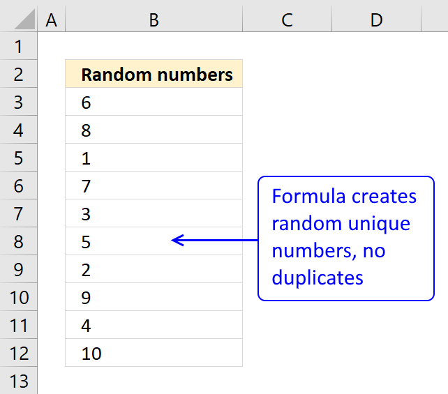
Question: How do I create a random list of unique numbers from say 1 to 10, without using VBA and without enabling iterative calculation in excel options and not using "helper" columns?
Answer:
The numbers in cell range A2:A11 are random and between 1 and 10.

Press function key F9 to generate a new random sequence.
Array formula in A2:
Excel 365 formula in cell A2:
How to enter an array formula
- Select cell A2
- Copy / Paste above array formula to formula bar
- Press and hold CTRL + SHIFT
- Press Enter
- Release all keys
Recommended articles

Array formulas allows you to do advanced calculations not possible with regular formulas.
Copy cell A2 and paste down as far as needed.
Explaining array formula in cell A2
Step 1 - Create an array
ROW($1:$10) creates this array {1, 2, 3, 4, 5, 6, 7, 8, 9, 10}
Step 2 - Create a criterion to avoid duplicate numbers
COUNTIF($A$1:A1, ROW($1:$10)) makes sure no duplicate numbers are created. The formula has both absolute and relative cell references ($A$1:A1). When the formula are copied down to cell A3 the cell reference changes to $A$1:A2. The value in cell A2 can´t be randomly selected again.
In cell A2, COUNTIF($A$1:A1, ROW($1:$10)) creates this array: {0, 0, 0, 0, 0, 0, 0, 0, 0, 0)
Recommended articles

Counts the number of cells that meet a specific condition.
Step 3 - Create a new dynamic array
ROW($1:$10)*NOT(COUNTIF($A$1:A1, ROW($1:$10))) creates this array in cell A2: {1, 2, 3, 4, 5, 6, 7, 8, 9, 10}
If the array formula randomly selects the number 2 in cell A2, the formula in cell A3 creates this array: {1, 0, 3, 4, 5, 6, 7, 8, 9, 10}
Number 2 can´t be selected anymore.
Step 4 - Calculate the number range in Randbetween(bottom, top)
The bottom value is always 1. The top value changes depending on current cell.
In cell A2 the top value is 10.
In cell A3 the top value is 9
and so on..
Formula in cell A2: 11-ROW(A1) equals 10. (11-1=10)
Formula in cell A3: 11-ROW(A2) equals 9. (11-2=9)
and so on..
Step 5 - Create a random number
=LARGE(ROW($1:$10)*NOT(COUNTIF($A$1:A1, ROW($1:$10))), RANDBETWEEN(1,11-ROW(A1)))
RANDBETWEEN(1,11-ROW(A1))
becomes
RANDBETWEEN(1,11-1)
becomes
RANDBETWEEN(1,10)
and returns a random number between 1 and 10.
Recommended articles
Microsoft Excel has three useful functions for generating random numbers, the RAND, RANDBETWEEN, and the RANDARRAY functions. The RAND function […]
Step 6 - Select a random number in array
=LARGE(ROW($1:$10)*NOT(COUNTIF($A$1:A1, ROW($1:$10))), RANDBETWEEN(1,11-ROW(A1)))
becomes
=LARGE({1, 2, 3, 4, 5, 6, 7, 8, 9, 10}, RANDBETWEEN(1,10))
becomes
=LARGE({1, 2, 3, 4, 5, 6, 7, 8, 9, 10}, random_number) and returns a random number between 1 and 10.
Recommended articles
The SMALL function lets you extract a number in a cell range based on how small it is compared to the other numbers in the group.
How to customize array formula to your excel work sheet
If your list starts at F3 change $A$1:A1 to $F$2:F2 in the above array formula. To change the numbers from 1 to 10 to, for example, 2 to 12, change $1:$10 to $2:$12 also in the above array formula.
Press F9 to generate a new random list of unique numbers.
23. Sort by week number

The image above shows a dynamic array formula that sorts values from cell range B3:C19 by the corresponding week number.
Formula in cell E3:
Step 1 - Calculate week number
The ISOWEEKNUM function calculates a number of the ISO week number of the year for a given date.
ISOWEEKNUM(B3:B19)
returns
{22; 22; 22; 43; 18; 28; 23; 13; 34; 12; 41; 46; 49; 20; 14; 49; 42}
Step 2 - Sort by week number
SORTBY(B3:C19, ISOWEEKNUM(B3:B19))
becomes
SORTBY(B3:C19, {22; 22; 22; 43; 18; 28; 23; 13; 34; 12; 41; 46; 49; 20; 14; 49; 42})
and returns
{43909,"Milena"; 43918,"Rogan"; 43924,"Paolo"; 43949,"Dolores"; 43968,"Kingsley"; 43976,"Rohan"; 43979,"Finlay"; 43976,"Sneha"; 43985,"Tyson"; 44018,"Leandro"; 44066,"Hasnain"; 44114,"Mai"; 44116,"Jane"; 44124,"Winifred"; 44149,"Collette"; 44169,"Manraj"; 44166,"Virginia"}.
24. Sort by quarter

The image above shows a dynamic array formula that calculates quarters based on dates in column B, it then sorts values from cell range B3:V19 by the quarters from small to large.
Formula in cell E3:
Step 1 - Calculate month number
The MONTH function returns a number from 1 to 12 from an Excel date representing the position. 1 - January, ... , 12 - December.
MONTH(B3:B19)
becomes
MONTH({43976; 43979; 43976; 44124; 43949; 44018; 43985; 43918; 44066; 43909; 44114; 44149; 44169; 43968; 43924; 44166; 44116})
and returns
{5; 5; 5; 10; 4; 7; 6; 3; 8; 3; 10; 11; 12; 5; 4; 12; 10}
Step 2 - Calculate quarter
The MATCH function returns a number representing the quarter, in this specific example.
MATCH(MONTH(B3:B19), {0;4;7;10}, 1)
becomes
MATCH({5; 5; 5; 10; 4; 7; 6; 3; 8; 3; 10; 11; 12; 5; 4; 12; 10}, {0;4;7;10}, 1)
and returns
{2; 2; 2; 4; 2; 3; 2; 1; 3; 1; 4; 4; 4; 2; 2; 4; 4}.
January -> 1 -> Quarter 1
February -> 2 -> Quarter 1
March -> 3 -> Quarter 1
April -> 4 -> Quarter 2
May -> 5 -> Quarter 2
June -> 6 -> Quarter 2
July -> 7 -> Quarter 3
August -> 8 -> Quarter 3
September -> 9 -> Quarter 3
October -> 10 -> Quarter 4
November -> 11 -> Quarter 4
December -> 12 -> Quarter 4
Step 3 - Sort by quarter
SORTBY(B3:C19, MATCH(MONTH(B3:B19), {0;4;7;10}, 1))
becomes
SORTBY(B3:C19, {2; 2; 2; 4; 2; 3; 2; 1; 3; 1; 4; 4; 4; 2; 2; 4; 4})
and returns
{43918,"Rogan"; 43909,"Milena"; 43976,"Rohan"; 43979,"Finlay"; 43976,"Sneha"; 43949,"Dolores"; 43985,"Tyson"; 43968,"Kingsley"; 43924,"Paolo"; 44018,"Leandro"; 44066,"Hasnain"; 44124,"Winifred"; 44114,"Mai"; 44149,"Collette"; 44169,"Manraj"; 44166,"Virginia"; 44116,"Jane"}
in cell F3.
25. Sort based on row count

The image above demonstrates a formula in cell E3 that extracts unique distinct rows from cell range B3:C11 sorted by row count.
For example, row 3 contains "Banana" and "20". Row 7 contains "Banana" and "20" as well, which makes the total row count 2 for that particular row.
The dynamic array formula in cell G3 returns 2 in cell G4 which corresponds to "Banana" and "20" in cell range E4:F4.
Formula in cell E3:
Step 1 - Count duplicate rows
The COUNTIFS function calculates the number of cells across multiple ranges that equals all given conditions.
COUNTIFS(criteria_range1, criteria1, [criteria_range2, criteria2]…)
We have two columns and must use two pairs of arguments to be able to count rows. The result is an array containing numbers for each corresponding row.
COUNTIFS(B3:B11, B3:B11, C3:C11, C3:C11)
becomes
COUNTIFS({"Banana"; "Lemon"; "Banana"; "Pear"; "Banana"; "Lemon"; "Banana"; "Lemon"; "Pear"}, {"Banana"; "Lemon"; "Banana"; "Pear"; "Banana"; "Lemon"; "Banana"; "Lemon"; "Pear"}, {20; 30; 10; 5; 20; 30; 10; 30; 10}, {20; 30; 10; 5; 20; 30; 10; 30; 10})
and returns {2; 3; 2; 1; 2; 3; 2; 3; 1}.

The first number in the array corresponds to the first row and so on. 2 means that there is a duplicate row in cell range B3:C11, the blue arrows show where that duplicate row is located.
Step 2 - Sort array based on row count
SORTBY(array, by_array1, [sort_order1], [by_array2, sort_order2],…)
The SORTBY function sorts values from cell range B3:C11 by the result array from the COUNTIFS function from large to small.
SORTBY(B3:C11, COUNTIFS(B3:B11, B3:B11, C3:C11, C3:C11), -1)
becomes
SORTBY(B3:C11, {2; 3; 2; 1; 2; 3; 2; 3; 1}, -1)
becomes
SORTBY({"Banana",20; "Lemon",30; "Banana",10; "Pear",5; "Banana",20; "Lemon",30; "Banana",10; "Lemon",30; "Pear",10}, {2; 3; 2; 1; 2; 3; 2; 3; 1}, -1)
and returns
{"Lemon",30; "Lemon",30; "Lemon",30; "Banana",20; "Banana",10; "Banana",20; "Banana",10; "Pear",5; "Pear",10}

Step 3 - Extract distinct rows
The UNIQUE function extracts unique distinct rows from the array.
UNIQUE(array,[by_col],[exactly_once])
UNIQUE(SORTBY(B3:C11, COUNTIFS(B3:B11, B3:B11, C3:C11, C3:C11), -1))
becomes
UNIQUE({"Lemon",30; "Lemon",30; "Lemon",30; "Banana",20; "Banana",10; "Banana",20; "Banana",10; "Pear",5; "Pear",10})
and returns
{"Lemon",30,3; "Banana",20,2; "Banana",10,2; "Pear",5,1; "Pear",10,1}
in cell E3.
Formula in cell G3:
I recommend a Pivot Table if you have a very large data set and experience a slow responding worksheet, it is lightning fast.
26. Sort numbers based on proximity to a given number

The image above demonstrates an array formula in cell C5 that sorts numbers, specified in cell range B5:B17, based on how far off they are from the given number in cell C2. Example, 9 and 11 are closest to 10 and are extracted first, displayed in cell C5 and C6.
Excel 365 formula:
Previous Excel versions:
27. Sort based on frequency row-wise

In this section, I will demonstrate two techniques for counting per row. The first example is simple and straightforward.
The second example is a bit more complicated but dynamic and automatic, you only need to provide a search string, everything else is calculated by array formulas.
What's on this section
- Count value per row
- Dynamic counting per row sorted from large to small
- Get Excel file
29.1. Count value per row

The first example has this data table, see image above. It is an Excel Table, select any cell in the data set and press CTRL + T to convert the data to an Excel Table.
I want to count the value "C" per row.
In cell J3, type:
Copy cell I2 and paste to I3:I10. You don't need to do this if you use an Excel Table as I did, see the image above. The Excel Table copies the formulas to cells below automatically.
The COUNTIF function counts the number of cells that meet a given condition.
There are 4 C's in row 2 so the formula returns 4 in cell J3. If you change the value in cell J2 to "B", the formulas in J3:J11 recalculates and return new values.
Let us sort the Excel table.
Drop-down list arrows appear next to each header, see picture above. Press with left mouse button on the arrow next to "C".

Press with left mouse button on "Largest to smallest". The data table shows the count of "C" per row, sorted largest to smallest.

Learn more about the COUNTIF function.
Do you know why $I$1 in COUNTIF(B2:H2,$I$1) has dollar signs?
Read this post: Absolute and relative cell references
29.2. Dynamic counting per row sorted from large to small

Now on to a more interesting and complicated example. The formula here returns names sorted in column E based on the number of "C"s per row.
How is this possible? The MMULT function is able to count cells per row based on a condition, it returns an array that corresponds to the number of rows. Change the value in cell C3 and the list in cell range E3:F11 is instantly changed.
I have applied conditional formatting to cell range B14:I22 so you can easily verify the calculated numbers in E3:E11.
Array formula in cell E3:
Excel 365 dynamic array formula in cell E3:
The formula above works only in Excel 365, it contains a new function: SORTBY.
Array formula in cell E3:
Explaining array formula in cell E3
Step 1 - Find search value in cell range
The equal sign compares the value in cell C3 to values in cell range c14:I22.
$C$14:$I$22=$C$3
becomes
{"C", "C", "B", "C", "C", "A", "B";"B", "B", "B", "C", "C", "C", "A";"C", "B", "B", "A", "A", "A", "A";"A", "B", "B", "C", "C", "C", "C";"A", "B", "C", "C", "C", "C", "B";"C", "B", "B", "A", "A", "C", "B";"A", "A", "C", "C", "C", "C", "B";"B", "A", "A", "A", "A", "B", "B";"B", "B", "A", "B", "A", "C", "B"}="C"
and returns
{TRUE, TRUE, FALSE, TRUE, TRUE, FALSE, FALSE;FALSE, FALSE, FALSE, TRUE, TRUE, TRUE, FALSE;TRUE, FALSE, FALSE, FALSE, FALSE, FALSE, FALSE;FALSE, FALSE, FALSE, TRUE, TRUE, TRUE, TRUE;FALSE, FALSE, TRUE, TRUE, TRUE, TRUE, FALSE;TRUE, FALSE, FALSE, FALSE, FALSE, TRUE, FALSE;FALSE, FALSE, TRUE, TRUE, TRUE, TRUE, FALSE;FALSE, FALSE, FALSE, FALSE, FALSE, FALSE, FALSE;FALSE, FALSE, FALSE, FALSE, FALSE, TRUE, FALSE}
Step 2 - Convert boolean values to numerical values
The parentheses lets you control the order of calculation, we want to compare $B$14:$H$22 with $B$3 before we multiply with 1.
($B$14:$H$22=$B$3)*1
becomes
{TRUE, TRUE, FALSE, TRUE, TRUE, FALSE, FALSE;FALSE, FALSE, FALSE, TRUE, TRUE, TRUE, FALSE;TRUE, FALSE, FALSE, FALSE, FALSE, FALSE, FALSE;FALSE, FALSE, FALSE, TRUE, TRUE, TRUE, TRUE;FALSE, FALSE, TRUE, TRUE, TRUE, TRUE, FALSE;TRUE, FALSE, FALSE, FALSE, FALSE, TRUE, FALSE;FALSE, FALSE, TRUE, TRUE, TRUE, TRUE, FALSE;FALSE, FALSE, FALSE, FALSE, FALSE, FALSE, FALSE;FALSE, FALSE, FALSE, FALSE, FALSE, TRUE, FALSE}*1
and returns
{1, 1, 0, 1, 1, 0, 0;0, 0, 0, 1, 1, 1, 0;1, 0, 0, 0, 0, 0, 0;0, 0, 0, 1, 1, 1, 1;0, 0, 1, 1, 1, 1, 0;1, 0, 0, 0, 0, 1, 0;0, 0, 1, 1, 1, 1, 0;0, 0, 0, 0, 0, 0, 0;0, 0, 0, 0, 0, 1, 0}.
Step 3 - Create an array containing corresponding column numbers
The COLUMN function returns the column number from a cell reference.
COLUMN($B$14:$H$22)
returns {2, 3, 4, 5, 6, 7, 8}.
Step 4 - Change numbers in array to 1
COLUMN($B$14:$H$22)^0
becomes
{2, 3, 4, 5, 6, 7, 8}^0
and returns {1, 1, 1, 1, 1, 1, 1}.
Step 5 - Evaluate MMULT function
The MMULT function calculates the matrix product of two arrays, an array as the same number of rows as array1 and columns as array2.
MMULT(($C$14:$I$22=$C$3)*1, TRANSPOSE(COLUMN($C$14:$I$22)^0))
becomes
MMULT({1, 1, 0, 1, 1, 0, 0;0, 0, 0, 1, 1, 1, 0;1, 0, 0, 0, 0, 0, 0;0, 0, 0, 1, 1, 1, 1;0, 0, 1, 1, 1, 1, 0;1, 0, 0, 0, 0, 1, 0;0, 0, 1, 1, 1, 1, 0;0, 0, 0, 0, 0, 0, 0;0, 0, 0, 0, 0, 1, 0}*1, {1, 1, 1, 1, 1, 1, 1})
and returns
{4; 3; 1; 4; 4; 2; 4; 0; 1}
Step 6 - Extract kth largest number
The LARGE function returns the kth largest number from a cell range or array.
LARGE(array, k)
LARGE(MMULT(($C$14:$I$22=$C$3)*1, TRANSPOSE(COLUMN($C$14:$I$22)^0)), ROWS($B$1:B1))
becomes
LARGE({4; 3; 1; 4; 4; 2; 4; 0; 1}, ROWS($B$1:B1))
The ROWS function returns a number representing the number of rows in a cell reference.
Cell reference $B$1:B1 grows when the cell is copied and pasted to cells below. This makes the ROWS function return a new number in each cell.
LARGE({4; 3; 1; 4; 4; 2; 4; 0; 1},1)
and returns 4.
Step 7 - Count values above the current cell
The COUNTIF function counts cells that equal a given condition. The cell reference $E$2:$E2 grows when the cell is copied and pasted to cells below, this lets the formula check all previous values.
COUNTIF($E$2:$E2, $B$14:$B$22)=0
becomes
{0;0;0;0;0;0;0;0;0}=0
and returns
{TRUE; TRUE; TRUE; TRUE; TRUE; TRUE; TRUE; TRUE; TRUE}
Step 8 - Filter count numbers based on previous values above
The IF function returns one value if the logical test is TRUE and another value if the logical test is FALSE.
IF(logical_test, [value_if_true], [value_if_false])
IF(COUNTIF($E$2:$E2, $B$14:$B$22)=0, MMULT(($C$14:$I$22=$C$3)*1, TRANSPOSE(COLUMN($C$14:$I$22)^0)), "")
becomes
IF({TRUE; TRUE; TRUE; TRUE; TRUE; TRUE; TRUE; TRUE; TRUE}, {4; 3; 1; 4; 4; 2; 4; 0; 1}, "")
and returns {4; 3; 1; 4; 4; 2; 4; 0; 1}.
Step 9 - Find the relative position of the kth largest number in the array
The MATCH function returns the relative position of an item in an array or cell reference that matches a specified value in a specific order.
MATCH(lookup_value, lookup_array, [match_type])
MATCH(LARGE(MMULT(($C$14:$I$22=$C$3)*1, TRANSPOSE(COLUMN($C$14:$I$22)^0)), ROWS($B$1:B1)), IF(COUNTIF($E$2:$E2, $B$14:$B$22)=0, MMULT(($C$14:$I$22=$C$3)*1, TRANSPOSE(COLUMN($C$14:$I$22)^0)), ""), 0)
becomes
MATCH(4, {4; 3; 1; 4; 4; 2; 4; 0; 1}, 0)
and returns 1.
Step 10 - Get value
The INDEX function returns a value from a cell range, you specify which value based on a row and column number.
INDEX($B$14:$B$22, MATCH(LARGE(MMULT(($C$14:$I$22=$C$3)*1, TRANSPOSE(COLUMN($C$14:$I$22)^0)), ROWS($B$1:B1)), IF(COUNTIF($E$2:$E2, $B$14:$B$22)=0, MMULT(($C$14:$I$22=$C$3)*1, TRANSPOSE(COLUMN($C$14:$I$22)^0)), ""), 0))
becomes
INDEX($B$14:$B$22, 1)
and returns "Wilhelm" in cell D3.
Check out: Dynamic scoreboard
29.3 Get Excel file
28. Sort by multiple columns using an Excel Table

The Excel Table is capable of sorting multiple columns in a specified order ascending and descending and which order sorting columns by. The image above shows buttons next to each column header name, next to the black triangle is a down-pointing arrow indicating that the column is sorted.
The image shows three down-pointing arrows, column J (PTS), I (GD) and G (GF). The table is sorted record by record based on the values in column J, I and G and in that order.
Convert data to an Excel Table

- Select any cell in the data set.
- Press CTRL + T to open the "Create Table" dialog box. See image above.
- Press with left mouse button on OK button.
Apply custom sort to an Excel Table

- Press with right mouse button on on any cell in the Excel Table.
- A pop-up menu appears, see image above. Press with left mouse button on or hover over "Sort".
- Another pop-up menu shows up, press with left mouse button on "Custom Sort...".
- A dialog box appears.

- Press with mouse on the first drop-down list, see image above.
- Press with mouse on the column header that you want to sort first by. I chose PTS.
- The "A to Z" drop-down list changed to "Smallest to Largest". Press with mouse on it to expand and see all drop-down list values.

- Press with mouse on "Largest to Smallest".
- Press with mouse on "Add Level" button.

- Now select the next column header name to sort by. I chose "GD".
- Repeat with the next column header name (GF).
- Press with left mouse button on OK button to apply settings.
29. Sort by multiple columns using the SORTBY function

Formula in cell B3:
The SORTBY function is available for Excel 365 subscribers, it has the following arguments:
SORTBY(array, by_array1, [sort_order1], [by_array2] , [sort_order2],…)
array - An array or cell reference to be sorted
by_array1 - An array or cell reference to be sorted on, this does not have to be a column in the array range. It can be a column outside the array range as well.
[sort_order1] - 1 for ascending, -1 for descending. Default value is -1 (ascending).
The arguments in brackets are optional arguments.
The formula above is a dynamic array formula meaning it spills values across columns and rows automatically.
Spilling is something dynamic array formulas do when they extend to adjacent cells as far as needed. The #SPILL! error is returned if a cell is not empty meaning dynamic array formulas will never overwrite populated cells.

As soon as you delete the contents of populated cells the dynamic array formula automatically extends to neighboring cells.
30. Sort by multiple columns using formula (Previous Excel versions)

The following formula sorts the table keeping the rows intact just like the above examples, the data source is in cell range B25:J44.
Array formula in cell B3:
How to enter an array formula in cell B3
- Copy the above formula.
- Double press with left mouse button on cell B3, a prompt appears in cell B3.
- Paste formula to the cell.
- Press and hold CTRL and SHIFT simultaneously.
- Press Enter once.
- Release all keys.
The formula begins and ends now with a curly bracket, like this: {=array_formula}
How to copy array formula
- Press with mouse on cell B3 to select it.
- Press CTRL + c to copy cell.
- Select cell range C3:J3.
- Paste to cell range C3:J3. CTRL + v.
- Select cell range B4:J22.
- Paste to cell range B4:J22. CTRL + v.
Explaining formula in cell B3

The "Evaluate Formula" tool allows you to troubleshoot and examine formulas in great detail. Go to tab "Formulas" on the ribbon. Press with mouse on "Evaluate Formula" button.
A dialog box appears, see image above. Press with left mouse button on the Evaluate button repeatedly to move through the calculation step by step.
Step 1 - Get points from column J
The following cell reference gets the points from the table.
$J$25:$J$44
returns
{48; 47; 46; 42; 41; 40; 37; 33; 30; 23; 23; 22; 21; 21; 20; 19; 18; 18; 17; 17}
Step 2 - Adjust negative numbers (GD) and divide with 1000
The Goal difference number can be negative, to adjust for that I am using the MIN function. The MIN function finds the smallest number in the cell range.
The ABS function removes the sign.
($I$25:$I$44+MIN($I$25:$I$44))/1000
becomes
({22; 36; 21; 25; 15; 1; 11; 2; 4; -5; -7; -13; -5; -5; -18; -24; -9; -19; -15; -18}+ABS(MIN($I$25:$I$44)))/1000
becomes
({22; 36; 21; 25; 15; 1; 11; 2; 4; -5; -7; -13; -5; -5; -18; -24; -9; -19; -15; -18}+ABS(MIN({22; 36; 21; 25; 15; 1; 11; 2; 4; -5; -7; -13; -5; -5; -18; -24; -9; -19; -15; -18})))/1000
becomes
({22; 36; 21; 25; 15; 1; 11; 2; 4; -5; -7; -13; -5; -5; -18; -24; -9; -19; -15; -18}+ABS(-24))/1000
becomes
({22; 36; 21; 25; 15; 1; 11; 2; 4; -5; -7; -13; -5; -5; -18; -24; -9; -19; -15; -18}+24)/1000
becomes
{46; 60; 45; 49; 39; 25; 35; 26; 28; 19; 17; 11; 19; 19; 6; 0; 15; 5; 9; 6}/1000
and returns
{0.046; 0.06; 0.045; 0.049; 0.039; 0.025; 0.035; 0.026; 0.028; 0.019; 0.017; 0.011; 0.019; 0.019; 0.006; 0; 0.015; 0.005; 0.009; 0.006}
Step 3 - Divide with 10000
We can't just add the goal difference to the points, that would destroy the sorting.
$G$25:$G$44/10000
becomes
{41; 20; 15; 40; 13; 34; 22; 22; 51; 59; 35; 29; 17; 27; 22; 19; 26; 26; 23; 21}/10000
and returns
{0.0041; 0.002; 0.0015; 0.004; 0.0013; 0.0034; 0.0022; 0.0022; 0.0051; 0.0059; 0.0035; 0.0029; 0.0017; 0.0027; 0.0022; 0.0019; 0.0026; 0.0026; 0.0023; 0.0021}
Step 4 - Add numbers
Step 4 adds the results from step to step 3.
$J$25:$J$44+($I$25:$I$44+MIN($I$25:$I$44))/1000+$G$25:$G$44/10000
becomes
{48; 47; 46; 42; 41; 40; 37; 33; 30; 23; 23; 22; 21; 21; 20; 19; 18; 18; 17; 17} + {0.046; 0.06; 0.045; 0.049; 0.039; 0.025; 0.035; 0.026; 0.028; 0.019; 0.017; 0.011; 0.019; 0.019; 0.006; 0; 0.015; 0.005; 0.009; 0.006} + {0.0041; 0.002; 0.0015; 0.004; 0.0013; 0.0034; 0.0022; 0.0022; 0.0051; 0.0059; 0.0035; 0.0029; 0.0017; 0.0027; 0.0022; 0.0019; 0.0026; 0.0026; 0.0023; 0.0021}
and returns
{48.0501; 47.062; 46.0465; 42.053; 41.0403; 40.0284; 37.0372; 33.0282; 30.0331; 23.0249; 23.0205; 22.0139; 21.0207; 21.0217; 20.0082; 19.0019; 18.0176; 18.0076; 17.0113; 17.0081}
Step 5 - Calculate k-th largest number
The LARGE function extracts the k-th largest number in an array or cell range. LARGE(array, k)
LARGE($J$25:$J$44+($I$25:$I$44+ABS(MIN($I$25:$I$44)))/1000+$G$25:$G$44/10000, ROWS($A$1:A1))
becomes
LARGE({48.0501; 47.062; 46.0465; 42.053; 41.0403; 40.0284; 37.0372; 33.0282; 30.0331; 23.0249; 23.0205; 22.0139; 21.0207; 21.0217; 20.0082; 19.0019; 18.0176; 18.0076; 17.0113; 17.0081}, ROWS($A$1:A1))
The ROWS function calculates the number of rows in a given cell reference. The cell reference in this case grows when we copy the cell and paste to cells below. This is possible if we use both an absolute and relative cell reference. This will return a new value in each cell.
LARGE({48.0501; 47.062; 46.0465; 42.053; 41.0403; 40.0284; 37.0372; 33.0282; 30.0331; 23.0249; 23.0205; 22.0139; 21.0207; 21.0217; 20.0082; 19.0019; 18.0176; 18.0076; 17.0113; 17.0081}, ROWS($A$1:A1))
becomes
LARGE({48.0501; 47.062; 46.0465; 42.053; 41.0403; 40.0284; 37.0372; 33.0282; 30.0331; 23.0249; 23.0205; 22.0139; 21.0207; 21.0217; 20.0082; 19.0019; 18.0176; 18.0076; 17.0113; 17.0081}, 1)
and returns
48.0501
Step 6 - Find relative position
The MATCH function calculates the relative position of a given value in a cell range or an array. MATCH(lookup_value, lookup_array, [match_type])
MATCH(LARGE($J$25:$J$44+($I$25:$I$44+ABS(MIN($I$25:$I$44)))/1000+$G$25:$G$44/10000, ROWS($A$1:A1)), $J$25:$J$44+($I$25:$I$44+ABS(MIN($I$25:$I$44)))/1000+$G$25:$G$44/10000, 0)
becomes
MATCH(48.0501, $J$25:$J$44+($I$25:$I$44+ABS(MIN($I$25:$I$44)))/1000+$G$25:$G$44/10000, 0)
becomes
MATCH(48.0501, {48.0501; 47.062; 46.0465; 42.053; 41.0403; 40.0284; 37.0372; 33.0282; 30.0331; 23.0249; 23.0205; 22.0139; 21.0207; 21.0217; 20.0082; 19.0019; 18.0176; 18.0076; 17.0113; 17.0081}, 0)
and returns 1.
Step 7 - Return value
The INDEX function returns a value based on a specified row and optional column number.
INDEX($B$25:$J$44, MATCH(LARGE($J$25:$J$44+($I$25:$I$44+ABS(MIN($I$25:$I$44)))/1000+$G$25:$G$44/10000, ROWS($A$1:A1)), $J$25:$J$44+($I$25:$I$44+ABS(MIN($I$25:$I$44)))/1000+$G$25:$G$44/10000, 0), COLUMNS($A$1:A1))
becomes
INDEX($B$25:$J$44, 1, COLUMNS($A$1:A1))
The COLUMNS function returns the number of columns in a given cell range. This will make the INDEX function return the correct value in each cell.
INDEX($B$25:$J$44, 1, COLUMNS($A$1:A1))
becomes
INDEX($B$25:$J$44, 1, 1)
and returns "Arsenal" in cell B3.
Recommended articles
Sort Two or More Columns (Contextures)
How to do a Multiple Level Data Sorting in Excel
'SORTBY' function examples
I will in this article discuss three different techniques to sort a data set in Excel. I am going to […]
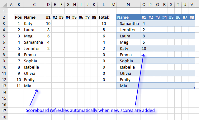
This article demonstrates a scoreboard, displayed to the left, that sorts contestants based on total scores and refreshes instantly each […]
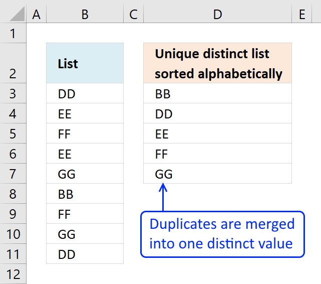
This article demonstrates Excel formulas that allows you to list unique distinct values from a single column and sort them […]
Functions in 'Lookup and reference' category
The SORTBY function function is one of 25 functions in the 'Lookup and reference' category.
Excel function categories
Excel categories
114 Responses to “How to use the SORTBY function”
Leave a Reply
How to comment
How to add a formula to your comment
<code>Insert your formula here.</code>
Convert less than and larger than signs
Use html character entities instead of less than and larger than signs.
< becomes < and > becomes >
How to add VBA code to your comment
[vb 1="vbnet" language=","]
Put your VBA code here.
[/vb]
How to add a picture to your comment:
Upload picture to postimage.org or imgur
Paste image link to your comment.
How to transpose it into colomn?
Fajar,
Array formula in B2:
Cell A2 is empty. Copy cell B2 to cell range C2:O2.
@ Oscar
Thank you for your quick reply.
Your suggestion is definitely work.
Thank you.
The sample file works in Excel 2003 while pressing F9, but if using F2 and ctrl+shift+enter on B3 for example, the result is #VALUE! even if not changing anything.
Formula evaluation shows in Step 5: RANDBETWEEN(1,{10}) with 10 in {} that evaluates to #VALUE.
As a workaround, I've added the first function that came to mind (SUM) to change the array with 1 item to a single value.
RANDBETWEEN(1,SUM(ROW(A1)))
Hallo, What if my number of rows will vary and I do not want to manually change the formula on different sheets?
Adell,
Array formula in cell B5:
You still have to adjust one cell range (bolded).
Thank you. I managed to get it working with using the Index and And function, pointing to my "count' value of maximum number required and it works like a charm!
I have some official user list which i want to use in random page number wise like attached example.
Please help me asap.
https://lh4.ggpht.com/1vrCVTerrixozegO8AyvQzUd7SNCWPeCv1oHKRUbJbIZ3UodpI_U8LdnvUs75yWPD3lanbc=s160
I have tried changing this formula to give me a random list of numbers from 1-189 but it doesn't work. Ideally what I want is a grid 15 by 27 full of numbers from 1-405. I was going to use this formula to give a list and paste them into my grid. Can anyone help?
mATT
Array formula in cell A2:
Copy cell A2 and paste to cell range A3:A190.
See attached file:
unique-random-list-of-numbers-1-189.xls
I know this post is a few years old. I need this exact solution, to randomly generate numbers without duplicates however in this case from 1 to 271. I have copied the above formula and the attached file to expand the range, though any modifications to either always results in #NUM error. Do you know why this is the case?
Following modified formula may help
={INDEX($B$17:$B$33, LARGE(MATCH(ROW($B$17:$B$33), ROW($B$17:$B$33))*NOT(COUNTIF($E$17:E21, $B$17:$B$33)), RANDBETWEEN(1, ROWS($B$17:$B$33)-COUNTA($E$17:E21))))}
Notice counta used at the end. This formula can be used starting from any row whereas the default one had to start at row 2.
Please note that you have to modify cell references since I have directly copied from relevant places in my excel sheet. Inconvenience regretted.
In formula counta function has been used in place of count since the purpose was to use this formula to generate random list of alphanumeric codes from list in a cell range.
I cannot seem to configure this formula to draw from an adjustable range taken from two cells.
Ex: I want a list of unique random numbers between whatever is entered in cell A4(Min) and B4(Max).
Any help would be greatly appreciated.
Array formula in cell B3:
See attached file:
unique-random-list-of-numbers-will.xls
Thank you Oscar. This only seems to work if the minimum is very low. Once you reach a minimum number>6 it begins to have problems. I am hoping to begin with numbers in the 1000-3000 range.
I wonder if you are seeing a similar problem?
Will,
you are right!
See attached file:
unique-random-list-of-numbers-will2.xls
This is brilliant Oscar. Thank you.
Thanks for this tip, but for some weird reason I still got a few duplicates. Is there a simple method to generate unique random numbers in a column?
I have a list of 1000 names in column A, and would like to generate unique integer numbers in column B for each of those names.
Thanks
My guess is that the cell reference (bolded below) is not changed.
=LARGE(ROW($1:$10)*NOT(COUNTIF($B$2:B2,ROW($1:$10))),RANDBETWEEN(1,11-ROW(A1)))
The array formula above is entered in cell range B3 and down as far as needed.
If you enter the formula in cell D4 and downwards, you must change the cell reference to $D$3:D3, like this:
=LARGE(ROW($1:$10)*NOT(COUNTIF($D$3:D3,ROW($1:$10))),RANDBETWEEN(1,11-ROW(A1)))
Hi Will,
This is a formula I used, the formula was in B3 down to B45 (teh length of my worksheet), the maximum was calcultated in B1, that is the formula revers to B1.
Hope it helps
{=LARGE(ROW(INDIRECT("$1:$"&B$1))*NOT(COUNTIF($B$2:B2,ROW(INDIRECT("$1:$"&B$1)))),RANDBETWEEN(1,B$1+1-ROW(B1))))}
Hi Will,
This formula i just posted, calculted, unique random numbers between 1 and X. Where the maksimum (X)changed on every schedule. My minimum is fixed at 1, but you can change the minimum to refer to a cell that indicated the minimum value/qty.
Good luck
Hi Adell,
I am having trouble changing the minimum value to anything but 1. It has a tendency to result in #NUM! or 0.
EX for 10-20 if B1=20:
{=LARGE(ROW(INDIRECT("$10:$"&B$1))*NOT(COUNTIF($B$2:B2,ROW(INDIRECT("$10:$"&B$1)))),RANDBETWEEN(10,$B$1+1-ROW(B1)))}
Can you tell me what I am doing wrong?
Thanks for all the help!
Hi Will,
The #num is usually, because you did not 'activate' the "string", that is the "{ }" in the beginning and end of the formula. Because there is more than one formula/statement that needs to be "true", before the calculation is done,you need to 'tell' excel to do 'all'. To do this (old fashioned way) you need to go to the beginning of your formula, before the "=" and hold down CTRL + SHFT + ENTER, then the "{}" will appear.
I had a look at the formula and have entered the minimum value into E2.
{=(LARGE(ROW(INDIRECT("$"&E$2&":$"&B$1))*NOT(COUNTIF($B$2:B2,ROW(INDIRECT("$"&E$2&":$"&B$1)))),RANDBETWEEN(E$2,B$1+1-ROW(B1))))}.
see the indirect sections as well as the randbetween part, where it stipulated the minimum and maximum values.
hope this helps, if not, shout :) (I don't know if you can obtain my email address from the webmaster if you need to contact me directly) (I am in RSA and will be going offline within the next hour - weekend! - and will only be back on Monday)
Adell
Will,
I also see that on your formula, you 'left out' the first and last set of brackets, that also might be part of your initial error.
=RANDBETWEEN(TIME(8,0,0),TIME(9,45,0))
i have to maintain random time between this nut is is not working
mayur,
randbetween works only with whole numbers.
Try this: =RAND()*(TIME(9,45,0)-TIME(8,0,0))+TIME(8,0,0)
Hi Frnd,
I want to get a random value between 1-20 but I not able to make any sucess ,I used the formula [=LARGE(ROW($1:$20)*NOT(COUNTIF($A$1:A1,ROW($1:$20))),RANDBETWEEN(1,21-ROW(A1)))]
But it is not working.Please help me...
Manoj,
your formula works, did you enter it as an array formula?
I tried on various systems with above code but i still get same error as below :
#NUM!
Please help me as it is very urgent for me.
Hi,
How to do tht or how do i make an array, because i tried as u guided above , please help me as it is very urgent
Hi ,
in your initial formula, you have "[". it should be "{". enter your formula, without the brackets before the "=" and the end one. Then, go to the beginning of your formula, to the left of the "=" and simultaneously press Ctrl Shft Enter . the "{" brackets will appear and your value will appear. (formula will work)
Hi,
I have done asu said but i get the error as: #VALUE!
and do not get the number ,please help
I used the below formula:
{=LARGE(ROW($1:$20)*NOT(COUNTIF($A$1:A1, ROW($1:$20))),RANDBETWEEN(1,21-ROW(A1)))}
Hi,
I have taken your formula, above and copied and pasted it into a new spreadsheet. took out the "{" and "}" and redid the CTRL SHFT ENTER to create the array/string formula and it works om my schedule. The only thing, that might through you out is the space between the comma and "ROW". go to the following link: https://speedy.sh/aMyaR/a.xlsx
You should be able to open it and see your formula working.
cheesh!.. sorry, it should be "throw you out" .... auto correct...
Hi ,
in your initial formula, you have "[". it should be "{". enter your formula, without the brackets before the "=" and the end one. Then, go to the beginning of your formula, to the left of the "=" and simultaneously press Ctrl Shft Enter . the "{" brackets will appear and your value will appear.
Hi,
I have done asu said but i get the error as: #VALUE!
and do not get the number ,please help
I used the below formula:
{=LARGE(ROW($1:$20)*NOT(COUNTIF($A$1:A1, ROW($1:$20))),RANDBETWEEN(1,21-ROW(A1)))}
Manoj,
Did you manage to get the spreadsheet I uploaded working? Is your formula working now?
Adell,
Thank you for yor support but I'm sorry as when I press with left mouse button on the given link from u ,I get security error n the the link closes n not allowing me to get the file . Is it possible for you sir to mail me the file on the following email id : [email protected]
Regards
Manoj
Hi Adell,
Is it possible to make a randome number set thro entire sheet: i tried the following formula :
[=LARGE(ROW($1:$65535)*NOT(COUNTIF($C$1:C1,ROW$1:$65535))),RANDBETWEEN(1,65536-ROW(C1)))]
but it seems not working:
whenever i try to edit your formulla n ammmend it according to my own chice , it gives error as "#NUM!" and when i pres ctrl+shift+enter , it gives this error "#VALUE!" , can you pls explain wht needs to be done to do it or can you pls make for me and send on : [email protected]
Thanks in advance.
Manoj,
You have a typo in your formula:
=LARGE(ROW($1:$65535)*NOT(COUNTIF($C$1:C1, ROW($1:$65535))), RANDBETWEEN(1, 65536-ROW(C1)))
I tried your formula and it works but it is extremely slow. Do you have to use formulas?
Also remember that the formula creates unique distinct random numbers. If you are looking for only random numbers use this:
=randbetween(0, 65535)
How can I make it start at 0? i.e. random numbers from 0 to 10?
=randbetween(0,10)
Can you try that? I tried that beforehand and it doesn't work for me. :( Why would 1,11 be 1-10 and 0,10 be 0 to 10?
I also want to have them lower down than rows 2-11 but can't make that work either. I tried changing the ROW($1:$10) bits but doesn't seem to work.
me,
try this formula in cell B3:
[...] An array formula taken from here..... How to create a list of random unique numbers in excel | Get Digital Help - Microsoft Excel resource [...]
[...] A couple of links that may help you: Learn Excel 2010 - "Random with No Repeats": Podcast #1471 - YouTube How to create a list of random unique numbers in excel | Get Digital Help - Microsoft Excel resource [...]
I've 30 objects and 10 people, and I need to assign each person with randomly (unique) selected objects as a daily activity. Would you please suggest me on how I can do it using excel formulae?
Vijay,
See this post: Assign each person with randomly unique objects as a daily activity
[...] Vijay asks: [...]
why does the code change the values in Columns "B" and "C" when I enter text values and tab to the next column?
This is what I'm Using, and I only want to affect Column "A" values:
=LARGE(ROW($1:$1000)*NOT(COUNTIF($A$1:A4, ROW($1:$1000))), RANDBETWEEN(1,1000-ROW(A4)))
Correction:
I should have copied the correct code (and lessened the number of tests):
=LARGE(ROW($1:$20)*NOT(COUNTIF($A$1:A1, ROW($1:$20))), RANDBETWEEN(1,20-ROW(A1)))
And, I should've said that when I enter a value in any other column, it automatically assigns a new random number to the fields in column "A". how to do I get it to assign a random number to column "A"'s fields without being readjusted when I enter any other information in the other columns???
Hi Paul,
Random numbers mean excel chooses a random number every time you refresh. (enter, tab, move etc)
Please give me more information as to what info do you want in A, B and C?
Regards
Adell,
I was looking for a way to have excel create a unique random number (not duplicated) in Column "A" that is not influenced by another key stroke. So, for instance, let's say I am creating a patient record and I want to give their account a uniqe number (almost like a primary key in Access or SQL). I don't want that number to be repeated, or to change as I enter more information in the next columns....
You might, once the number has randomly been created make it a definite number and not a formula anymore by: copy, paste special, values.
Or, for a patient number, for instance is to use say the first 3 letters of their surname [use this formula is the surname is in column B =LEFT(B2,3)] with a number, starting at 00001 to infinity. Have excel check that this combination has not been used before?
Let me know if this would work for you.
I think the second option, in using the first 3 letters of the surname with a random number may be the best option in this case. How would you recommend going about doing that???
Paul,
Perhaps like this:
As per Oscar's formula, your numbers will be sequential, which is great, for record keeping and all rules and regulations, that I have ever come in contact with, regarding assigning of record numbers. If you combine your random number formula in stead of the countif formula, you will still have the issue of the numbers changing every time, unless you copy/paste/special after assigning a number. Good luck
Hi Oscar,
Excellent article - with the steps explained.
Only I could not understand why the randbetween is restricted to lesser and lesser values as the range progresses.
RANDBETWEEN(1,20-ROW(A1)))
Request you to explain the logic.
Oscar -
Trying to convert this into a formula for creating a random list from another source. For example, if I have a list of the 50 U.S. states I'd like to create a random/unique list of x number of states. I'm using the position of the state in the INDEX to use as the random number but I'm having trouble in the COUNTIF statement to relate the prior state names I've returned to the "used" portion of the COUNTIF array.
GMF,
Generate unique random text strings
In Excel 2003, when I copy your formula into the formula bar, (cell A2), and use CTRL-SHIFT-ENTER, I get #VALUE! for a result. When I copy the cell directly from your worksheet, (in that case cell B3), and paste it into a blank worksheet, it works fine. Examining that formula it shows #VALUE! for 'RANDBETWEEN(1,11-ROW(A1))', but still works. If I press with left mouse button on the formula bar and then CTRL-SHIFT-ENTER, that formula stops working and returns #VALUE!. I can work around it by replacing ROW(A1) by 1, ROW(A2) by 2, etc.; or 11-ROW(A1) by 10,,etc. – but for sanity's sake, I would like to know what Excel magic you use to make your formula work. Thanks.
Hi Oscar,
I am trying to create a random list of of ten one digit numbers between 0 and 9. It gives me a formula error when I try to do it. Any assistance would be greatly appreciated.
Regards,
Gavin
Gavin,
Did you enter the formula as an array formula? (Instructions above)
Hi All,
Would really appreciate it if someone can help me.
I am trying to generate random numbers between -300 & 300.
The formula above seems to work for positive numbers only?
=LARGE(ROW($1:$300)*NOT(COUNTIF($A$1:A1, ROW($1:$300))), RANDBETWEEN(1,300-ROW(A1)))
How can I make this formula generate negative and positive ( -300 to 300)
Thanks
Jack,
Yes, you are right.
Try this:
=LARGE(ROW($1:$600)*NOT(COUNTIF($A$1:A1, ROW($1:$600))), RANDBETWEEN(1,600-ROW(A1)))-300
Thanks Oscar you are the best.
I tried it but some numbers are omitted and others are repeated. Would it be okay to email you directly?
Thank you so much
Jack
Jack,
Sorry, you are right. Try this in cell A2:
=LARGE(ROW($1:$600)*NOT(COUNTIF($A$1:A1, ROW($1:$600)-300)), RANDBETWEEN(1,600-ROW(A1)))-300
If this isn´t working, email me.
I am trying to generate a random sequence of 1-10 without duplicates, but I would like to separate the numbers into two parts such that the first 5 numbers are a random sequence of 1-5 and the last 5 numbers are a random sequence of 6-10. (So the random sequence would look like this for example: 3 2 4 1 5 / 9 8 6 10 7) Is this possible to do with a formula? Do you have any suggestions?
Thank you.
Amy,
I am afraid no, but it is possible with a custom function (vba).
Hey,
For some reason I'm having trouble transposing these formulas for my needs.
I need 2 sets of random numbers in a spreadsheet, if possible 0-9 (not 1-10)
One set starting in cell C2 and going across the columns to L2
The other set starting in B3 and going down to B12
Thanks!
I need two sets of 10 random numbers between 0 and 9 (included) if 0 isn't an option then 1-10 is ok...
cell ranges are C2:L2 and B3:B12
Any help would be much appreciated!
Actually make those cell ranges C3:L3 and B4:B14. Sorry just having trouble with this
Hello, how I can generate 100 random numbers from 11111 up to 55555, but the numbers must be unique and not contain (0,6,7,8,9)
Daniel,
I am not sure you can do that with an array formula. You need a custom function (vba).
Can you help me?
Thank you so much for this simple solution. It's been the final piece in creating a differentiated started for practicing mental calculations in maths. Here's the result: https://lttmaths.com/2014/02/16/differentiated-mental-calculation-strategy-starter/
Nyima,
I am happy you found it useful. I have made something similar before:
https://www.get-digital-help.com/basic-mathematics-in-excel-for-school-children/
[…] produces calculations suitable for each strategy (and looking on the web for methods to produce unique random numbers in Microsoft Excel - apparently harder than it first sounds!) Also included is a MENTAL TEST SCORE SHEET to record […]
I would like to produce a list of random numbers (non repeating). the number needs to be 5 digits. The number cannot start with zero. So it can have all the digits 0 - 9 in it but cannot start with zero. How do I do this?
leslie,
Try this array formula in cell A2:
=LARGE(ROW($10000:$99999)*NOT(COUNTIF($A$1:A1, ROW($10000:$99999))), RANDBETWEEN(1,89999-ROW(A1)))
Remember to adjust the bolded cell reference if you enter the array formula in another cell.
Oscar, thank you very much. I ended up entering the formula to generate 5,000 numbers ($1000:$5999) but it took forever. My computer is new with plenty of processing ability so does it make sense that this took a long time. Furthermore, once it was complete I copied the column from that spreadsheet to another one and did a paste special value and it took 2 hours to paste. At then end of it though I have the 5,000 numbers.
Hi, Excellent description on how to use Excell.
However I'm attempting to generate 8 unique random numbers along a row ranging from 1-45. I have tried using your combination of your reply to fajar and the generate values from a cell range however I do not understand how to convert it to go across (along the row) not down (down the column)
Any help would be greatly appreciated!
When copying the formula to cell A2 Excel reports an error in COUNTIF($A$1:A1) pointing to A1 as the source. Any ideas?
Thanks.
Patrick.
Patrick,
Enter the formula in cell A2, not in cell A1. Then copy cell A2 to the cells below.
Genius thanks. I did notice that when modifying to get 30 unique numbers from a range 1-32 the number 1 is rare. Still trying to get my head round this. Also if I type into other columns it regenerates the values.
Hello,
I created the barcodes using a font type, but when I cannot read it with my barcode scanner Motorola MC3090. I've also tried with others barcodes for example, with a notebook and It works for it. What am I doing wrong? I have to write down and additional formula?
Thanks a lot for your help
Need assistance with random number. I'm dealing with service tickets in an excel sheet to generate a report for demo data.
I need to use the =TIMEVALUE("2:00:00") or go off of the original ticket time in the row, for instance. 6/6/2014 1:02:00 AM.
I would need to explain via web session or phone call. I'd be willing to pay $$ if someone wanted to help me.
How do you extrapolate the formula to make a unique table of numbers?
1.0302
1.0310
13.1910
1.0101
13.1310
9.0902
1.0310
9.0902
1.0302
1.0102
13.1310
13.1917
13.1317
13.1310
13.1317
9.0902
1.0302
1.0310
9.0902
13.1317
Ab0ve r my total ranks,but the final rank i got with COUNTIF($AC$2:$AC$21,"<"&AC)+1 is 1 for all!!
Hasan,
I believe you have entered this formula as an array formula:
COUNTIF($AC$2:$AC$21,"<"&AC)+1 It is a regular formula, press enter only and then copy it down as far as needed.
Hi,
I am trying to use the "unique random text strings" to make random pairs of students in my classroom. However: I have opened the attached example file, and while it works perfectly when I open it (I press F9 and get the states randomly sorted again and again), whenever I access the formula I get the #N/A error. I am on Excel 2007, norwegian language pack. All I have to do is press with my mouse in the formula line (like if I wanted to edit the formula) and press enter, and I get error.
What is it that changes when I try to edit the formula?
Thx
edit: I'm an idiot.
Remember to use ctrl+shift+enter instead of just enter when editing array files...
Please let me know if you're looking for a author foor your blog.
You have some really gokod posts and I feel I would be a good
asset. If you ever want to take some of thhe load off,
I'd really like to write some material for your blog iin exchanbge for a link back
to mine.Please blasat me an emil if interested. Kudos!
Hi I am trying to figure out how to use the array formula you supplied in the excel Unique random text strings... My list is a bit longer but I am unable to make changes to the formula. I keep getting error when I would like to make the ROW to 100. Yours stops at 52.
I might need more coffee but I can't seem to figure this out... Can you help?
Thanks in advance. Jennifer
Thank you so much for your help!
Hi, i am wanting to make a table of riders for random gates to start a race. There is 8 riders per race in 8 lanes and am trying to avoid riders getting the same lane.
Thanks in advance
First Name- ratul
Last Name- roy
Date of birth - 19/02/1987
I want a automated calculation in excel which print VP19021987RRAA
RR- first word of first name(Ratul-R) and first word of last name (Roy-R)
19021987- date of birth
AA- I want that value will automatically change when the same value will come that is VP19021987RRAA to VP19021987RRAB
Please help me
Hi Oscar,
I tryed to calculate stanging just from results. For example: we have two teams A and B and we know results between them and want to calculate wins, draws, loses, points and goal difference.
A : B
2 : 1 = wins for A
2 : 2 = draw
2 : 3 = lose for A
1 : 0
3 : 1
1 : 4
Logic is simple, but I failed to find a way to calculate without helper columns
[…] How to create a list of random unique numbers in excel … – Table of Contents. Generate unique random numbers; Generate unique random values from a cell range; Generate unique random numbers. Question: How do I create a random … […]
RAND() function in Excel makes Ctrl+y stop working. Why?
[…] How to create a list of random unique numbers in excel […]
Oscar,
I really appreciate that you make the formula very simple to make ranking format.
But i'm little bit confused about the number you've choose as denominator
for Rank GD AND Rank GF . Can you please elaborate more for me.
And i'm also looking for answer for two more condition ;
if we consider " Concerned teams (Pnt, GF-GA, GF)" for 2nd step and
Coefficient rank for the 5th step.
then what would be the formula ?
If you may please help me out of this prob.
looking forward to your kind co-operation.
Thanks
Hi,
I have a cell, A1. And I want to use random number generator to get an array basead on the number inside A1.
So let's say A1 is 2. the array i want is 2, 2+1, 2+2, 2+3 spread between A2~A5 randomly.
Is that possible?
Hi,
If you are going to use the sort function at the end to rank then why not use it on the whole table like:
Sort J by smallest to Largest
Add another Level
Sort G by Largest to smallest
And another level
Sort H by Largest to smallest
Add another Level
Sort I by Largest to smallest
Marq
Yes, you are right.
I am looking to create a excel with serial numbers as example "121417-ASX-WER-THX"
I am using the Table insertion to autogenerate the serial number when a new row is added but unable to get the above serial number. Please help.
DREAM 11 TEAM GENERATOR IF TOTAL 100 /AND HOW MANY TEAM WILL GET 100 CREDITPOINTS
9 TEAM OR 8 TEAM
AUTOMATIC GENERATOR
Hello,
Excellent and very complete explanation ... !!!
For all non-365 users, is there a possible replicate ?
Could an Array Formula handle the Sort by a column of numbers and generate the same result as the basic Sortby function ?
Thanks in advance for your insight
James,
yes it is possible.
Formula in cell E3:
Array formula in cell F3:
Hello Oscar,
Thanks a lot ...!!!
This is an encouragement for me to have the full SIX Dynamic Array Functions that Microsoft has decided NOT to offer to the Legacy Excel Users ... replicated either in Array Formulas or with UDFs.
Only a few hundreds of Millions Excel loyal users are now left with no updates ... !!!
For sure, they do not deserve any attention ... since they have already paid their license.
Thanks again for your help and for your site which is a great great resource !!!
Take Care
James