How to use the AVERAGE function
What is the AVERAGE function?
The AVERAGE function calculates the average of numbers in a cell range. In other words, the sum of a group of numbers and then dividing by the count of those numbers.
Table of Contents
- Syntax
- Arguments
- Example
- Column containing some text values
- Are zeros counted?
- Are boolean values ignored?
- Absolute values
- Across sheets - 3D range
- By group
- By month
- Blank as zero
- Excluding high and low
- Exclude some cells
- Calculate running average of last 10 data with random blank cells
- Get Excel *.xlsx file
- Example - ignore blanks
- Example - ignore NA()
- Example - based on criteria
- Function not working
1. Syntax
The AVERAGE function may have up to 255 arguments, each argument can contain a reference to a single cell, cell range, and/or constants.
You can also use other functions in the arguments, this makes it possible to calculate an average based on a condition or criteria among many other things.
AVERAGE(number1, [number2], ...)
2. Arguments
The first argument is required, the remaining arguments are optional.
number1 - Required. numbers or a cell range
[number2] - Optional. Additional arguments up to 255
3. Example
![]()
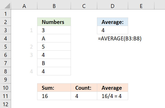
This example demonstrates a formula in cell D3 that calculates an average based on a column, the column contains both numerical values and empty cells.
This is not a problem, the AVERAGE function is designed to ignore empty blank cells.
Formula in cell D3:
Cells B4 and B7 are empty, they are not counted. 3 + 5 + 4 + 4 equals 16. 16 / 4 equals 4.
Here is how the AVERAGE function works:

4. How to average a column containing some text values
This example demonstrates a formula in cell D3 that calculates an average based on a column, the column contains both numerical values and text values.
This is also not a problem, the AVERAGE function is designed to ignore text values, however, keep in mind that error values are not ignored.
Formula in cell D3:
Cells B4 and B7 are empty, they are not counted. 3 + 5 + 4 + 4 equals 16. 16 / 4 equals 4.
5. Are zeros included?
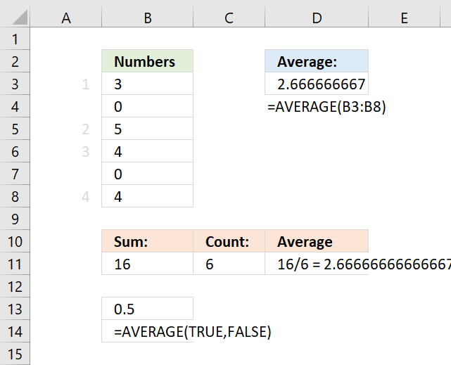
This example demonstrates a formula in cell D3 that calculates an average based on values located in a column, the column contains numerical values including some zeros.
The AVERAGE function calculates an average including zeros by default. How to calculate an average and ignore 0 (zeros)
Formula in cell D3:
Cells B4 and B7 are empty, they are not counted. 3 + 5 + 4 + 4 equals 16. 16 / 4 equals 4.
Cells B4 and B7 contain 0 (zeros), they are counted.
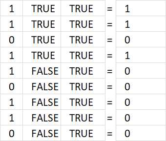
6. Are boolean values ignored?

Boolean values in a cell range are ignored and not counted shown in cell D3 in the example above.
Formula in cell D3:
3 + 5 + 4 + 4 = 16. 16/4 = 4.

Boolean values are ignored by the AVERAGE function, however, they are included if you enter a boolean value as a constant in an argument, see cell B13 above.
The numerical equivalents are:
TRUE = 1
FALSE = 0 (zero)
Formula in cell B13:
1 + 0 = 1. 1/2 = 0.5 Cell B13 returns 0.5.

To average boolean values multiply the cell range with 1, this converts boolean values to their numerical equivalent.
Array formula in cell D6:
6.1 How to enter an array formula

To enter an array formula, type the formula in a cell then press and hold CTRL + SHIFT simultaneously, now press Enter once. Release all keys.
The formula bar now shows the formula with a beginning and ending curly bracket telling you that you entered the formula successfully. Don't enter the curly brackets yourself.
6.2 Explaining formula in cell D6
Step 1 - Convert boolean values
B3:B8*1
becomes
{3; TRUE; 5; 4; TRUE; 4}*1
and returns
{3; 1; 5; 4; 1; 4}.
Step 2 - Calculate the average
AVERAGE(B3:B8*1)
becomes
AVERAGE({3; 1; 5; 4; 1; 4})
and returns 3. 3 + 1 + 5 + 4 + 1 + 4 = 18. 18/6 = 3.
7. How to average absolute values

The array formula in cell D3 converts numbers in B3:B8 to absolute numbers meaning the minus sign is removed. In other words, all numbers are equal to 0 (zero) or larger. The numbers are 3, -2, 5, -3, 3, and 4.
Formula in cell D3:
3 + 2 + 5 + 3 + 3 + 4 equals 20. 20 / 6 = approx. 3.33
8. Explaining formula
Step 1 - Calculate positive numbers
The ABS function converts negative numbers to positive numbers, in other words, the ABS function removes the sign.
ABS(number)
ABS(B3:B8)
becomes
ABS({3; -2; 5; -3; 3; 4})
and returns
{3; 2; 5; 3; 3; 4}.
Step 2 - Calculate the average
AVERAGE(ABS(B3:B8))
becomes
AVERAGE({3; 2; 5; 3; 3; 4})
and returns approx. 3.33
8. How to calculate an average across sheets

In order to calculate an average across worksheets values must be located at the same cell range throughout all worksheets. This technique can greatly reduce time you need to spend on formulas.
Formula in cell D3:
The formula uses values from sheets 'Across sheets' and 'Across sheets1' in both cell ranges B3:B8 and returns approx. 3.167
Here is how to enter this formula:
- Double press with left mouse button on cell D3, the prompt appears.
- Type =AVERAGE(
- Select cell range B3:B8 with mouse.
- Select tab "Across sheets" with left mouse button.
- Press and hold SHIFT key.
- Select tab "Across sheets1" with left mouse button.
- Release SHIFT key.
- Type )
- Press Enter.
All worksheets between Across sheets and Across sheets1 are now selected This example has only these two worksheets however, the technique is the same regardless the number of worksheets.
9. How to average by group

The image above demonstrates an array formula that calculates an average based on a condition specified in cell F2. Cell range B3:B8 contains categories and cell range C3:C8 contains the corresponding numbers we want to calculate an average.
Array formula in cell D3:
The array formula in cell D3 extracts number 3, 5, 3, and 4 based on the corresponding categories on the same row in cell range B3:B8. The average is 3.75 and here is how:
3+5+3+4 equals 15.
15 / 4 equals 3.75 This value matches the value in cell D3, our calculations are correct.
Explaining formula
Step 1 - Logical test
The equal sign lets you compare value to value, the result is a boolean value TRUE or FALSE. This will tell us which cells are equal to the condition.
B3:B8=F2 becomes {"A"; "B"; "A"; "B"; "A"; "A"}="A"
and returns {TRUE; FALSE; TRUE; FALSE; TRUE; TRUE}.
Step 2 - Evaluate IF function
The IF function returns one value if the logical test is TRUE and another value if the logical test is FALSE.
IF(logical_test, [value_if_true], [value_if_false])
IF(B3:B8=F2,C3:C8,"") becomes IF({TRUE; FALSE; TRUE; FALSE; TRUE; TRUE},C3:C8,"")
becomes IF({TRUE; FALSE; TRUE; FALSE; TRUE; TRUE},{3; -2; 5; -3; 3; 4},"")
and returns {3; ""; 5; ""; 3; 4}.
Step 3 - Calculate average
AVERAGE(IF(B3:B8=F2,C3:C8,"")) becomes AVERAGE({3; ""; 5; ""; 3; 4}) and returns 3.75
Note, the AVERAGEIF and AVERAGEIFS functions are built to handle conditions without the need for an array formula. They are available for Excel 2007 users and later versions, I highly recommend you check them out.
10. How to calculate an average based on a month in corresponding date on the same row

This example lets you calculate an average based on the month in corresponding dates. The image above shows dates in cell range B3:B8, the months are B3: January, B4: February, B5: January, B6: March, B7 and B8: January.
The condition is specified in cell F2. 1 is January, 2 i February ... 12 is December. The formula filters the numbers in C3:C8 based on the dates in B3:B8 if the dates are equal to 1 meaning January.
Array formula in cell F4:
The number is not included in the calculation if the corresponding date is not equal to the specified value in cell F2 which is 1 in this example.
Explaining formula
Step 1 - Calculate month number
The MONTH function returns a number corresponding to the position of a given month in a year. January = 1, ... December = 12.
MONTH(B3:B8)
becomes
MONTH({44583; 44611; 44564; 44635; 44579; 44572})
and returns
{1; 2; 1; 3; 1; 1}.
Step 2 - Identify numbers equal to the specified month
The equal sign lets you compare value to value, the result is a boolean value TRUE or FALSE. This will tell us which cells are equal to the condition.
MONTH(B3:B8)=F2
becomes
{1; 2; 1; 3; 1; 1}=F2
becomes
{1; 2; 1; 3; 1; 1}=1
and returns
{TRUE; FALSE; TRUE; FALSE; TRUE; TRUE}.
Step 3 - Replace TRUE with corresponding number in C3:C8
The IF function returns one value if the logical test is TRUE and another value if the logical test is FALSE.
IF(logical_test, [value_if_true], [value_if_false])
IF(MONTH(B3:B8)=F2,C3:C8,"")
becomes
IF({TRUE; FALSE; TRUE; FALSE; TRUE; TRUE}, C3:C8, "")
becomes
IF({TRUE; FALSE; TRUE; FALSE; TRUE; TRUE}, {3; -2; 5; -3; 3; 4}, "")
and returns
{3; ""; 5; ""; 3; 4}.
Step 4 - Calculate average
AVERAGE(IF(MONTH(B3:B8)=F2,C3:C8,""))
becomes
AVERAGE({3; ""; 5; ""; 3; 4})
and returns 3.75
3 + 5 + 3 + 4 = 15. 15/4 = 3.75
11. How to average blank as zero

The AVERAGE function ignores blank cells , however, there is a simple workaround that allows you to count 0's (zeros) to the total number of observations.
Keep in mind, the average is calculated like this: Sum / total number of items. A blank cell is not in the total they are simply ignored. The trick is to add a 0 to the cell range, this makes the formula add a zero to a blank cell which returns a 0 (zero) in all blank cells in the given cell range.
Array formula in cell E4:
There are occasions when you want the blank to be counted in the total number of items and this is how to do it in the regular AVERAGE function. This is simple, reliable and effective.
Explaining formula
Step 1 - Add 0 (zero) to values
The plus sign lets you add numbers in Excel, an empty cell converts to a 0 (zero).
B3:B8+0
becomes
{3; ""; 5; ""; 3; 4} + 0
and returns {3; 0; 5; 0; 3; 4}.
Step 2 - Calculate average
AVERAGE(B3:B8+0)
becomes
AVERAGE({3; 0; 5; 0; 3; 4})
and returns 2.5
3+0+5+0+3+4 = 15. 15/6 = 2.5
Average without blanks as zeros: 3+5+3+4 = 15. 15/4 = 3.75
12. How to calculate an average excluding the largest and smallest numbers

This example demonstrates a formula that excludes the largest and smallest number from a set of values. The image above shows six values in cell range B3:B8 and they are: 3, 2, 5, 2, 1, and 4.
The formula excludes the highest and lowest number from the calculations, if there are multiple values matching the largest or smallest value then all of them are excluded.
Array formula in cell E2:
The largest number in 3, 2, 5, 2, 1, and 4 is 5 and the smallest is 1, The remaining values are 3, 2, 2, and 4. 3+2+2+4 equals 11. 11 / 4 equals 2.75
Explaining formula
Step 1 - Calculate the largest value
The MAX function returns the largest value in a cell range or array.
MAX(number1, [number2], ...)
MAX(B3:B8)
becomes
MAX({3; 2; 5; 2; 1; 4})
and returns 5.
Step 2 - Compare largest value to B3:B8
The equal sign lets you compare value to value, the result is a boolean value TRUE or FALSE. This will tell us which cells are equal to the largest number.
MAX(B3:B8)=B3:B8
becomes
5={3; 2; 5; 2; 1; 4}
and returns
{FALSE; FALSE; TRUE; FALSE; FALSE; FALSE}.
Step 3 - Calculate smallest value
The MIN function returns the smallest number in cell range or array.
MIN(number1, [number2], ...)
MIN(B3:B8)
becomes
MIN({3; 2; 5; 2; 1; 4})
and returns 1.
Step 4 - Compare the smallest number to numbers in B3:B8
The equal sign lets you compare value to value, the result is a boolean value TRUE or FALSE. This will tell us which cells are equal to the smallest number.
MIN(B3:B8)=B3:B8
becomes
1= {3; 2; 5; 2; 1; 4}
and returns
{FALSE; FALSE; FALSE; FALSE; TRUE; FALSE}.
Step 5 - Add arrays (OR logic)
The plus sign lets you add values and also arrays, this creates OR logic between the two arrays containing boolean values.
TRUE + TRUE = TRUE
TRUE + FALSE = TRUE
FALSE + TRUE = TRUE
FALSE + FALSE = FALSE
One more thing, the boolean values are converted into their numerical equivalents when you add the arrays.
TRUE = 1 or in fact any number except zero
FALSE = 0 (zero)
(MAX(B3:B8)=B3:B8)+(MIN(B3:B8)=B3:B8)
becomes
{FALSE; FALSE; TRUE; FALSE; FALSE; FALSE} + {FALSE; FALSE; FALSE; FALSE; TRUE; FALSE}
and returns {0; 0; 1; 0; 1; 0}.
Step 6 - Replace 0 (zero) with corresponding value
The IF function returns one value if the logical test is TRUE and another value if the logical test is FALSE.
IF(logical_test, [value_if_true], [value_if_false])
IF((MAX(B3:B8)=B3:B8)+(MIN(B3:B8)=B3:B8),"",B3:B8)
becomes
IF({0; 0; 1; 0; 1; 0},"",B3:B8)
becomes
IF({0; 0; 1; 0; 1; 0},"", {3; 2; 5; 2; 1; 4})
and returns {3; 2; ""; 2; ""; 4}.
Step 7 - Calculate average
AVERAGE(IF((MAX(B3:B8)=B3:B8)+(MIN(B3:B8)=B3:B8),"",B3:B8))
becomes
AVERAGE({3; 2; ""; 2; ""; 4})
and returns 2.75
3 +2 + 2 + 4 = 11. 11/4 = 2.75
13. How to exclude some cells from average

This formula calculates an average based on numbers in cell range B3:B8, however, only if they are not also in the exclude list in cell range D3:D5.
For example, the numbers in cell range B3:B8 are 3, 2, 5, 1, 3, and 4. The numbers in the exclude list are 2, 3, and 4. The remaining values in cell range B3:B8 are 5 and 1.
The average becomes 5 + 1 equals 6. 6 / 2 eqials 3.
Array formula in cell F3:
The formula is small, easy to adjust and easy to understand. Excel 365 users may enter this array formula as a regular formula.
Explaining formula
Step 1 - Identify numbers based on criteria
The COUNTIF function calculates the number of cells that is equal to a condition. This will tell us where the excluded cells are.
COUNTIF(range, criteria)
COUNTIF(D3:D5, B3:B8)
becomes
COUNTIF({2;3;4},{3;2;5;1;3;4})
and returns
{1; 1; 0; 0; 1; 1}.
Step 2 - Replace 1 with nothing and 0 (zero) with number
The IF function returns one value if the logical test is TRUE and another value if the logical test is FALSE.
IF(logical_test, [value_if_true], [value_if_false])
IF(COUNTIF(D3:D5, B3:B8), "", B3:B8)
becomes
IF({1; 1; 0; 0; 1; 1}, "", B3:B8)
becomes
IF({1; 1; 0; 0; 1; 1}, "", {3; 2; 5; 1; 3; 4})
and returns
{""; ""; 5; 1; ""; ""}.
Step 3 - Calculate average
AVERAGE(IF(COUNTIF(D3:D5, B3:B8), "", B3:B8))
becomes
AVERAGE({""; ""; 5; 1; ""; ""})
and returns 3. 5+1 = 6. 6/2 = 3
14. Calculate running average of last 10 data with random blank cells
![]()
Question:
- List of data and blank cells in a column which will be added from day to day.
- There are sometimes blank cells in column.
How to get the average of the 10 most recent data? The average will change from day to day.
Answer:
This array formula creates a dynamic range, filtering the 10 last data and returns the average. Adjust cell ranges $A$1:$A$25 in formula below.
Array formula in cell C3:
How to create an array formula
Excel 365 users can skip these steps, no need to enter an array formula. Simply press Enter.
- Select cell C3
- Copy (Ctrl + c) array formula
- Paste (Ctrl + v) array formula to formula bar.
- Press and hold Ctrl + Shift simultaneously.
- Press Enter once.
- Release all keys.
How this array formula works in cell C18
The array formula calculates a dynamic cell range in column C to use based on non-empty cells in column B. $B$3:B3 is a dynamic cell reference, it expands as you copy the formula to cells below. This makes it a running average meaning a new average is calculated in every new cell below cell C.
The INDEX function creates a cell reference based on the 10th largest row number calculated from the non-empty cells in column B. This cell reference changes dynamically making it possible to calculate a running average.
The LARGE function tries to find the 10th largest row number. The LARGE function returns an error before 10 non empty cells are found and the IFERROR function converts the errors to a "hyphen". This is why you see hyphen or a minus character in the first top cells in column C.
As soon as there are 10 values in column B to average the formula returns the calculated value. This continues as far as you copy the formula to cells below and have values in column B.
The difference between this formula and other running calculations is that it actually checks that there are 10 values to process. It also calculates the 10 last values based on the current cell ignoring blanks. Earlier values are not in the calculation, you can change this to any number. To do this change 10 in the formula to the number of values you want to calculate an average of.
Step 1 - Extract row numbers of not empty cells
The IF function has three arguments, the first one must be a logical expression. If the expression evaluates to TRUE then one thing happens (argument 2) and if FALSE another thing happens (argument 3).
The logical expression contains an expanding cell range that grows when the cell is copied to cells below.
IF($B$3:B18<>"", ROW($B$3:B18), "")
becomes
IF({TRUE; FALSE; TRUE; FALSE; TRUE; TRUE; TRUE; TRUE; FALSE; FALSE; FALSE; TRUE; TRUE; FALSE; TRUE; TRUE}, ROW($B$3:B18), "")
becomes
IF({TRUE; FALSE; TRUE; FALSE; TRUE; TRUE; TRUE; TRUE; FALSE; FALSE; FALSE; TRUE; TRUE; FALSE; TRUE; TRUE}, {3; 4; 5; 6; 7; 8; 9; 10; 11; 12; 13; 14; 15; 16; 17; 18}, "")
and returns {3;"";5;"";7;8;9;10;"";"";"";14;15;"";17;18}.
Step 2 - Calculate the 10th largest row number
The LARGE function returns the k-th largest number. LARGE( array, k)
LARGE(IF($B$3:B18<>"", ROW($B$3:B18), ""), 10)
becomes
LARGE({3;"";5;"";7;8;9;10;"";"";"";14;15;"";17;18}, 10)
and returns 3.
Step 3 - Use row number to create a cell reference
The INDEX function lets you build a cell reference based on a row and column number.
INDEX(B:B, LARGE(IF($B$3:B3<>"", ROW($B$3:B3), ""), 10))
becomes
INDEX(B:B, 3)
and returns B3.
Step 4 - Build complete cell reference
A cell reference may contain two parts separated by a colon.
INDEX(B:B, LARGE(IF($B$3:B3<>"", ROW($B$3:B3), ""), 10)):B18
returns B3:B18.
Step 5 - Average values
The AVERAGE function calculates the average based on the cell reference we calculated earlier.
AVERAGE(INDEX(B:B, LARGE(IF($B$3:B3<>"", ROW($B$3:B3), ""), 10)):B18)
becomes
AVERAGE(B3:B18)
and returns 53.8
Step 6 - Return - if calculation returns error
The IFERROR fucntion returns "-" if the formula returns an error which it does until 10 numbers are found in the cell range.
Get Excel *.xlsx file
Useful resources
AVERAGE function - Microsoft
How To Calculate the Average of a Group of Numbers
16. AVERAGE ignore blanks
![]()
Table of Contents
- AVERAGE ignore blanks
- Average - ignore blanks and errors
- Average - ignore blanks in non-contiguous cells
- Weighted average ignore blanks
- Average ignore 0 (zeros) and blanks
- Get Excel *.xlsx file
16.1. AVERAGE ignore blanks
![]()
The AVERAGE function is designed to ignore blank cells automatically but there are instances where it fails. The picture above seems to have blank cells in B3:B8, however, they are counted as zeros. Why?
16.1.1 Cells containing 0 (zero) formatted as a blank
The cells in B3:B8 are not truly empty, select B3:B8 and press CTRL + 1 to open the "Format Cells" settings.
![]()
Here we see that it has been formatted with custom cell formatting. Values containing 0 (zeros) are hidden, to show them press with left mouse button on General and then OK.
This will show your zeros again on your worksheet, if not read the next section. If you are interested in learning more about custom formatting codes, read this article: Excel’s TEXT function explained
16.1.2 Check your Excel settings
If this didn't do it, go to your Excel Options and then press with left mouse button on "Advanced".
Excel 2016 Users press with left mouse button on "File" on the ribbon and then press with left mouse button on "Options".
![]()
Find "Show a zero in cells that have zero value", is it enabled?
16.2. Average - ignore blanks and errors

The AVERAGE function ignores empty cells out of the box automatically, no need to worry about that. However, if you are working with possible error values and use the IFERROR function to handle errors strange things happen.
The IFERROR function removes errors but has this side effect that it converts blank cells to zeros which in turn makes the AVERAGE function return an incorrect result.
Try this formula: =AVERAGE(IFERROR(B3:B8, "")) it returns 2 if you use the example values above and that is wrong. Use instead the following formula.
Formula in cell D3:
The formula above converts blank cells to error value #N/A! and then remove the error values, here are the steps in detail:
Explaining formula
Step 1 - Identify nonempty cells
The less than and the greater than signs combined evaluate to "not equal to", in this case, not equal to nothing (blank). The result is a boolean value TRUE or FALSE.
B3:B8<>""'
returns {TRUE; TRUE; #DIV/0!; FALSE; #N/A; TRUE}.
Step 2 - Replace empty values with an error value
The IF function returns one value if the logical test is TRUE and another value if the logical test is FALSE.
IF(logical_test, [value_if_true], [value_if_false])
The IF function replaces TRUE with the corresponding value and FALSE with an error value. Error values in the logical test expression return the same in the IF function.
IF(B3:B8<>"", B3:B8, NA())
returns {5; #N/A; #DIV/0!; #N/A; #N/A; 1},
Step 3 - Handle error values
The IFERROR function replaces error values with a given value that you specify.
IFERROR(value, value_if_error)
In this case it replaces error values with nothing (blank).
IFERROR(IF(B3:B8<>"",B3:B8,NA()),"")
returns {5; ""; ""; ""; ""; 1}.
Step 4 - Calculate the average
The AVERAGE function calculates the average of a group of numbers, text and blank cells are ignored.
AVERAGE(number1, [number2], ...)
AVERAGE(IFERROR(IF(B3:B8<>"",B3:B8,NA()),""))
returns 3 in cell D3. 5 + 1 = 6. 6 / 2 = 3.
16.3. Average - ignore blanks in non-contiguous cells

The following formula contains two non contiguous cell ranges B3:B8 and D3:D4, the AVERAGE function ignores blank cells automatically. If this is not the case, make sure Excel isn't using a different cell formatting, see section 1.1 and 1.2 above.
Formula in cell B11:
5+3+1+5 = 14. 14/4 = 3.5
16.4. Weighted average ignore blanks

Formula in cell C14:
16.4.1 Explaining formula in cell C14
Step 1 - Find weight based on value
The LOOKUP function lets you find a value in a cell range and return a corresponding value on the same row.
LOOKUP(lookup_value, lookup_vector, [result_vector])
LOOKUP($B$3:$B$12, $E$3:$E$8, F3:F8)
returns {1; 3; 6; 4; 4; 1; 1; 5; 4; 4}.
Step 2 - Replace blank values with 0 (zero)
The IF function returns one value if the logical test is TRUE and another value if the logical test is FALSE.
IF(logical_test, [value_if_true], [value_if_false])
IF(B3:B12<>"", LOOKUP($B$3:$B$12, $E$3:$E$8, F3:F8), 0)
returns {0; 3; 6; 4; 4; 1; 0; 5; 4; 4}.
Step 3 - Multiply array with weights
IF(B3:B12<>"", LOOKUP($B$3:$B$12, $E$3:$E$8, F3:F8), 0)*C3:C12
returns {0; 120; 180; 360; 320; 20; 0; 50; 40; 160}.
Step 4 - Add numbers and return a total
The SUMPRODUCT function calculates the product of corresponding values and then returns the sum of each multiplication.
SUMPRODUCT(IF(B3:B12<>"", LOOKUP($B$3:$B$12, $E$3:$E$8, F3:F8), 0)*C3:C12)
returns 1250.
Step 5 - Calculate the total weight
The SUM function calculates a sum based on a cell range or array.
SUM(IF(B3:B12<>"", LOOKUP($B$3:$B$12, $E$3:$E$8, F3:F8), 0)
returns 31.
Step 6 - Divide total by total weight
SUMPRODUCT(IF(B3:B12<>"", LOOKUP($B$3:$B$12, $E$3:$E$8, F3:F8), 0)*C3:C12)/SUM(IF(B3:B12<>"", LOOKUP($B$3:$B$12, $E$3:$E$8, F3:F8), 0))
returns 40.3225806451613.
16.5. Average ignore 0 (zero) and blanks

The AVERAGE function ignores empty cells automatically. If this is not the case, make sure Excel isn't using a different cell formatting, see section 1.1 and 1.2 above.
Formula in cell B11:
5+3+1=9. 9/3 = 3
16.6 Get Excel *.xlsx file
17. AVERAGE ignore NA()
The AVERAGE function ignores empty cells, text values, and boolean values automatically, however, it doesn't handle error values. The AVERAGE function returns an error if the data contains at least one error value.
This article describes a few different workarounds to this problem based on the Excel version you are using. Cell range C3:C9 contains some random numbers and a few #N/A errors, I will use this data to demonstrate a few formulas that can help you out.
Table of Contents
- AVERAGE function can't handle errors
- AVERAGE ignore NA() - Excel 2007 and later versions
- AVERAGE ignore NA() - earlier versions
- AVERAGE ignore #N/A for non-contiguous cell ranges
- Get Excel *.xlsx file
17.1. AVERAGE function can't handle errors

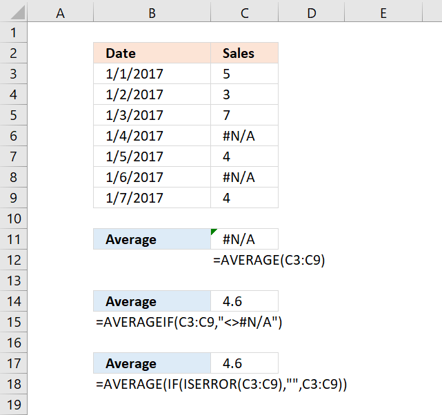
#N/A error is sometimes used to show gaps in charts, however, the AVERAGE function can't handle errors, shown in C11 in the picture above.
Formula in cell C11:
Evaluate formula
Step 1 - Populate function
The AVERAGE function calculates the average of numbers in a cell range. In other words, the sum of a group of numbers and then divided by the count of those numbers.
AVERAGE(number1, [number2], ...)
AVERAGE(C3:C9)
becomes
AVERAGE({5; 3; 7; #N/A; 4; #N/A; 4})
Note that cell reference C3:C9 evaluates to an array with a beginning and ending curly bracket. Values are delimited by a semicolon meaning the values are arranged horizontally.
Your Excel software may show something else than the semicolon, it is determined by your regional settings.
Notice the error value #N/A is displayed in two locations in the array, they correspond to the values in cell C3:C9.
Step 2 - Calculate the average
AVERAGE({5; 3; 7; #N/A; 4; #N/A; 4})
returns #N/A. This shows that the AVERAGE function can't ignore error values, you need to somehow handle this using other functions.
17.2. AVERAGE ignore NA() - Excel 2007 and later versions

There is an easy workaround, the AVERAGEIF function allows you to ignore #N/A errors. It was introduced in Excel 2007.
Explaining formula
Step 1 - Populate arguments
The AVERAGEIF function returns the average of cell values that are valid for a given condition.
AVERAGEIF(range, criteria, [average_range])
range - C3:C9
criteria - "<>#N/A"
[average_range] - empty
The larger and smaller than signs are the same as "not equal to".
Step 2 - Evaluate AVERAGEIF function
AVERAGEIF(C3:C9,"<>#N/A")
returns 4.6
17.3. AVERAGE ignore NA() - earlier versions
If you have an Excel version earlier than 2007, the ISERROR function works just as fine. The downside is that you need to enter the formula as an array formula.
Array formula in cell C17:
17.3.1 How to enter an array formula
To enter an array formula, type the formula in a cell then press and hold CTRL + SHIFT simultaneously, now press Enter once. Release all keys.
The formula bar now shows the formula with a beginning and ending curly bracket telling you that you entered the formula successfully. Don't enter the curly brackets yourself.
17.3.2 Explaining formula
Step 1 - Identify error values
The ISERROR function returns TRUE if a value is an error value.
ISERROR(value)
ISERROR(C3:C9)
returns {FALSE; FALSE; FALSE; TRUE; FALSE; TRUE; FALSE}
Step 2 - Replace FALSE with corresponding number
The IF function returns one value if the logical test is TRUE and another value if the logical test is FALSE.
IF(logical_test, [value_if_true], [value_if_false])
IF(ISERROR(C3:C9),"",C3:C9)
returns {5; 3; 7; ""; 4; ""; 4}.
Step 3 - Calculate average
The AVERAGE function calculates the average of numbers in a cell range. In other words, the sum of a group of numbers and then divided by the count of those numbers.
AVERAGE(number1, [number2], ...)
AVERAGE(IF(ISERROR(C3:C9),"",{5; 3; 7; #N/A; 4; #N/A; 4}))
returns 4.6
17.4. AVERAGE ignore #N/A for non-contiguous cell ranges

The image above demonstrates a formula that calculates an average based on two non-contiguous ranges and ignores error values.
Array formula in cell C11:
17.4.1 Explaining array formula in cell C11
Step 1 - Handle errors in C3:C9
The IFERROR function lets you catch most errors in Excel formulas, it lets you specify a new value replacing the old error value.
IFERROR(value, value_if_error)
IFERROR(C3:C9,"")
returns {5; 3; 7; ""; 4; ""; 4}.
Step 2 - Handle errors in E3:E9
IFERROR(E3:E9,"")
returns {11; 10; 16; ""; 13; ""; 15}
Step 3 - Calculate average
The AVERAGE function calculates the average of numbers in a cell range. In other words, the sum of a group of numbers and then divided by the count of those numbers.
AVERAGE(number1, [number2], ...)
AVERAGE(IFERROR(C3:C9,""),IFERROR(E3:E9,""))
returns 8.8
17.5 Get Excel *.xlsx file
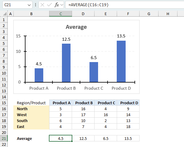
18. AVERAGE based on criteria
This section demonstrates two formulas that calculate averages, the first formula calculates an average based on criteria, and the second formula uses both criteria and two other conditions applied to an adjacent column using AND logic.
What's on this section
- AVERAGE based on criteria
- AVERAGE - AND OR logic
- Get Excel *.xlsx file
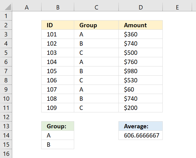
18.1. AVERAGE based on criteria
The array formula in cell D14 calculates an average based on multiple criteria in cell range B14:B15. If value in column C is equal to B14 or B15 the amount in column D on the same row is included in the average.
18.1.1 How to enter an array formula
To enter an array formula, type the formula in a cell then press and hold CTRL + SHIFT simultaneously, now press Enter once. Release all keys.
The formula bar now shows the formula with a beginning and ending curly bracket telling you that you entered the formula successfully. Don't enter the curly brackets yourself.
18.1.2 Explaining formula in cell D14
Step 1 - Count cells based on criteria
You can't use AVERAGEIF or AVERAGEIFS function in this example, as far as I know. The COUNTIF function allows you to check if at least one out of multiple values are found in a cell range.
Note that I am using multiple values in the second argument, the COUNTIF function returns an array that indicates where group A or B is.
COUNTIF(range, criteria)
COUNTIF(B14:B15, C3:C11)
becomes
COUNTIF({"A";"B"},{"A";"B";"C";"A";"B";"C";"B";"B";"C"})
and returns {1; 1; 0; 1; 1; 0; 1; 1; 0}. The image below shows the array next to column Amount.
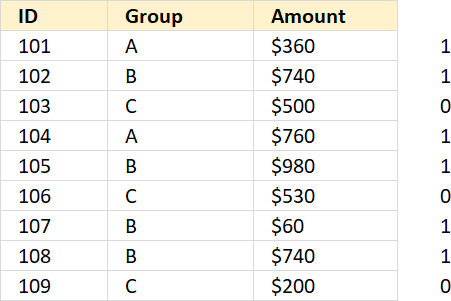
If group is "A" or "B" the corresponding cell on the same row is 1 in the column without a name (next to column Amount).
Step 2 - Replace 1 with the corresponding amount
The IF function lets you filter values in column D based on the COUNTIF function that serves as a logical test in this case.
IF(logical_test, [value_if_true], [value_if_false])
IF(COUNTIF(B14:B15, C3:C11), D3:D11, "")
becomes
IF({1; 1; 0; 1; 1; 0; 1; 1; 0}, D3:D11, "")
and returns
{360; 740; ""; 760; 980; ""; 60; 740; ""}
Step 3 - Calculate average
The AVERAGE function then returns the average from the values in the array ignoring the blanks.
AVERAGE(number1, [number2], ...)
AVERAGE(IF(COUNTIF(B14:B15,C3:C11),D3:D11,""))
becomes
AVERAGE({360;740;"";760;980;"";60;740;""})
returns 606.6667 in cell D14.
18.2. AVERAGE - AND OR logic
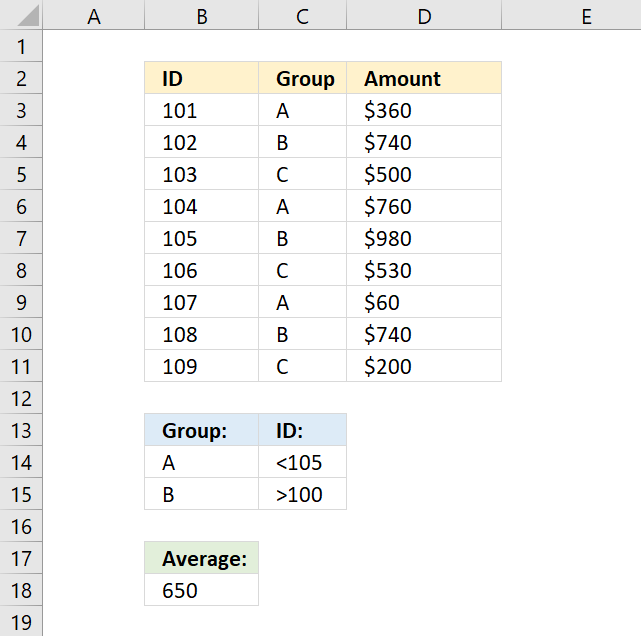
The following array formula calculates an average based on two conditions, if group is equal to A OR B AND ID is less than 105 AND larger than 100.
18.2.1 Explaining formula
Step 1 - First condition
The COUNTIF function allows you to check if at least one out of multiple values are found in a cell range.
Note that I am using multiple values in the second argument, the COUNTIF function returns an array that indicates where group A or B is.
COUNTIF(range, criteria)
COUNTIF(B14:B15, C3:C11)
becomes
COUNTIF({"A"; "B"},{"A"; "B"; "C"; "A"; "B"; "C"; "A"; "B"; "C"})
and returns {1; 1; 0; 1; 1; 0; 1; 1; 0}.
Step 2 - Second condition
The less than character is a logical operator that checks if the numbers in B3:B11 are smaller than 105, the result is a boolean value TRUE or FALSE.
B3:B11<105
becomes
{101; 102; 103; 104; 105; 106; 107; 108; 109}<105
and returns
{TRUE; TRUE; TRUE; TRUE; FALSE; FALSE; FALSE; FALSE; FALSE}.
Step 3 - Third condition
The greater than character is a logical operator that checks if the numbers in B3:B11 are larger than 100.
B3:B11>100
becomes
{101; 102; 103; 104; 105; 106; 107; 108; 109}>100
and returns
{TRUE; TRUE; TRUE; TRUE; TRUE; TRUE; TRUE; TRUE; TRUE}.
Step 4 - Multiply arrays
There are three logical expressions in the first IF argument COUNTIF(B14:B15,C3:C11)*(B3:B11<105)*(B3:B11>100).
The asterisk multiplies the arrays, 1 indicates a location where all three logical tests return TRUE and FALSE if at least one returns FALSE.
The array returned from the COUNTIF function is in the first column above, B3:B11<105 is in the second column, and B3:B11>100 is in the third column.
The first row: 1*TRUE*TRUE equals 1. All three logical tests are TRUE.
COUNTIF(B14:B15, C3:C11)*(B3:B11<105)*(B3:B11>100)
becomes
{1; 1; 0; 1; 1; 0; 1; 1; 0}*{TRUE; TRUE; TRUE; TRUE; FALSE; FALSE; FALSE; FALSE; FALSE}*{TRUE; TRUE; TRUE; TRUE; TRUE; TRUE; TRUE; TRUE; TRUE}
and returns
{1; 1; 0; 1; 0; 0; 0; 0; 0}.
Step 5 - Replace 1 with the corresponding amount
The IF function lets you filter values in column D based on the COUNTIF function that serves as a logical test in this case.
IF(logical_test, [value_if_true], [value_if_false])
The corresponding value on the same row is 360 and is included in the AVERAGE calculation.
IF(COUNTIF(B14:B15, C3:C11)*(B3:B11<105)*(B3:B11>100), D3:D11,"")
becomes
IF({1; 1; 0; 1; 0; 0; 0; 0; 0}, D3:D11,"")
becomes
IF({1; 1; 0; 1; 0; 0; 0; 0; 0}, {360; 740; 500; 760; 980; 530; 60; 740; 200},"")
and returns
{360; 740; ""; 760; ""; ""; ""; ""; ""}.
Step 6 - Calculate average
The AVERAGE function then returns the average from the values in the array ignoring the blanks.
AVERAGE(number1, [number2], ...)
AVERAGE(IF(COUNTIF(B14:B15, C3:C11)*(B3:B11<105)*(B3:B11>100), D3:D11,""))
becomes
AVERAGE({360; 740; ""; 760; ""; ""; ""; ""; ""})
There are two more values that are also in the calculation found in the second and fourth row, 740 and 760.
The average is 620 and is displayed in cell B18.
18.3. Get Excel *.xlsx file
AVERAGE based on multiple criteria
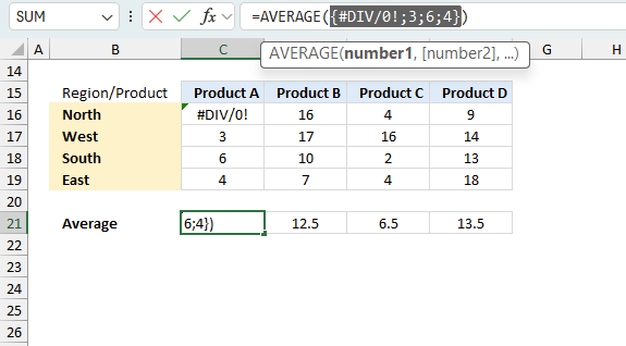
19. Function not working
The AVERAGE function returns
- #NAME? error if you misspell the function name.
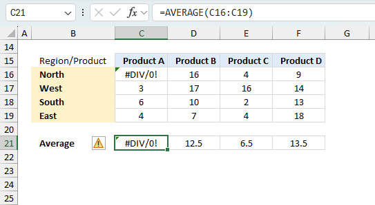
- propagates errors, meaning that if the input contains an error (e.g., #VALUE!, #REF!, #DIV/0!), the function will return the same error.
19.1 Troubleshooting the error value
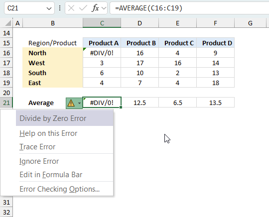
When you encounter an error value in a cell a warning symbol appears, displayed in the image above. Press with mouse on it to see a pop-up menu that lets you get more information about the error.
- The first line describes the error if you press with left mouse button on it.
- The second line opens a pane that explains the error in greater detail.
- The third line takes you to the "Evaluate Formula" tool, a dialog box appears allowing you to examine the formula in greater detail.
- This line lets you ignore the error value meaning the warning icon disappears, however, the error is still in the cell.
- The fifth line lets you edit the formula in the Formula bar.
- The sixth line opens the Excel settings so you can adjust the Error Checking Options.
Here are a few of the most common Excel errors you may encounter.
#NULL error - This error occurs most often if you by mistake use a space character in a formula where it shouldn't be. Excel interprets a space character as an intersection operator. If the ranges don't intersect an #NULL error is returned. The #NULL! error occurs when a formula attempts to calculate the intersection of two ranges that do not actually intersect. This can happen when the wrong range operator is used in the formula, or when the intersection operator (represented by a space character) is used between two ranges that do not overlap. To fix this error double check that the ranges referenced in the formula that use the intersection operator actually have cells in common.
#SPILL error - The #SPILL! error occurs only in version Excel 365 and is caused by a dynamic array being to large, meaning there are cells below and/or to the right that are not empty. This prevents the dynamic array formula expanding into new empty cells.
#DIV/0 error - This error happens if you try to divide a number by 0 (zero) or a value that equates to zero which is not possible mathematically.
#VALUE error - The #VALUE error occurs when a formula has a value that is of the wrong data type. Such as text where a number is expected or when dates are evaluated as text.
#REF error - The #REF error happens when a cell reference is invalid. This can happen if a cell is deleted that is referenced by a formula.
#NAME error - The #NAME error happens if you misspelled a function or a named range.
#NUM error - The #NUM error shows up when you try to use invalid numeric values in formulas, like square root of a negative number.
#N/A error - The #N/A error happens when a value is not available for a formula or found in a given cell range, for example in the VLOOKUP or MATCH functions.
#GETTING_DATA error - The #GETTING_DATA error shows while external sources are loading, this can indicate a delay in fetching the data or that the external source is unavailable right now.
19.2 The formula returns an unexpected value
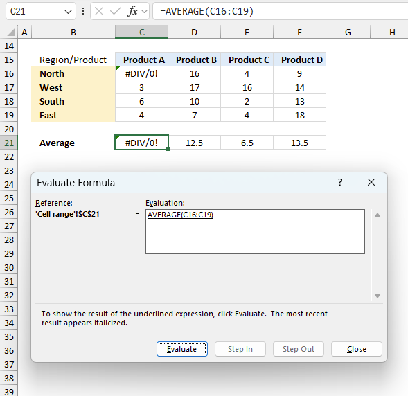
To understand why a formula returns an unexpected value we need to examine the calculations steps in detail. Luckily, Excel has a tool that is really handy in these situations. Here is how to troubleshoot a formula:
- Select the cell containing the formula you want to examine in detail.
- Go to tab “Formulas” on the ribbon.
- Press with left mouse button on "Evaluate Formula" button. A dialog box appears.
The formula appears in a white field inside the dialog box. Underlined expressions are calculations being processed in the next step. The italicized expression is the most recent result. The buttons at the bottom of the dialog box allows you to evaluate the formula in smaller calculations which you control. - Press with left mouse button on the "Evaluate" button located at the bottom of the dialog box to process the underlined expression.
- Repeat pressing the "Evaluate" button until you have seen all calculations step by step. This allows you to examine the formula in greater detail and hopefully find the culprit.
- Press "Close" button to dismiss the dialog box.
There is also another way to debug formulas using the function key F9. F9 is especially useful if you have a feeling that a specific part of the formula is the issue, this makes it faster than the "Evaluate Formula" tool since you don't need to go through all calculations to find the issue.
- Enter Edit mode: Double-press with left mouse button on the cell or press F2 to enter Edit mode for the formula.
- Select part of the formula: Highlight the specific part of the formula you want to evaluate. You can select and evaluate any part of the formula that could work as a standalone formula.
- Press F9: This will calculate and display the result of just that selected portion.
- Evaluate step-by-step: You can select and evaluate different parts of the formula to see intermediate results.
- Check for errors: This allows you to pinpoint which part of a complex formula may be causing an error.
The image above shows cell reference C16:C19 converted to hard-coded value using the F9 key. The AVERAGE function requires numerical values between 0 (zero) and 1 which is not the case in this example. We have found what is wrong with the formula.
Tips!
- View actual values: Selecting a cell reference and pressing F9 will show the actual values in those cells.
- Exit safely: Press Esc to exit Edit mode without changing the formula. Don't press Enter, as that would replace the formula part with the calculated value.
- Full recalculation: Pressing F9 outside of Edit mode will recalculate all formulas in the workbook.
Remember to be careful not to accidentally overwrite parts of your formula when using F9. Always exit with Esc rather than Enter to preserve the original formula. However, if you make a mistake overwriting the formula it is not the end of the world. You can “undo” the action by pressing keyboard shortcut keys CTRL + z or pressing the “Undo” button
19.3 Other errors
Floating-point arithmetic may give inaccurate results in Excel - Article
Floating-point errors are usually very small, often beyond the 15th decimal place, and in most cases don't affect calculations significantly.
'AVERAGE' function examples
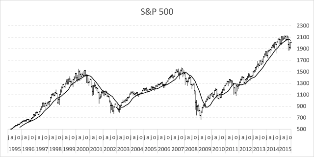
In my previous post, I described how to build a dynamic stock chart that lets you easily adjust the date […]
Functions in 'Statistical' category
The AVERAGE function function is one of 73 functions in the 'Statistical' category.
Excel function categories
Excel categories
25 Responses to “How to use the AVERAGE function”
Leave a Reply
How to comment
How to add a formula to your comment
<code>Insert your formula here.</code>
Convert less than and larger than signs
Use html character entities instead of less than and larger than signs.
< becomes < and > becomes >
How to add VBA code to your comment
[vb 1="vbnet" language=","]
Put your VBA code here.
[/vb]
How to add a picture to your comment:
Upload picture to postimage.org or imgur
Paste image link to your comment.
Oscar, what if list of data and blank cells are in a row.
Let's say data starts from Column C.
Cyril,
Array formula:
Yes, this CSE would average the last 10 Columns. But it would include the blanks.
Cyril,
Yes, the formula includes the ten last values. But the blanks are not counted and calculated?
Given the example posted above that is {1;"" ; 2;"" ; 2; 3; 4; 5;"" ;"" ;"" ; 6; 7;"" ; 8; 9;"" ; 10;"" ;"" ; 11; 12; 13;"" ; 14}, the average of the last 10 values (integers) would be 9.5.
Given that the data are in Row 1 from Column I to AG.
Given the formula in D1 as follows =AVERAGE(INDEX(I1:AG1, LARGE(IF($I$1:$AG$1"", COLUMN($I$1:$AG$1), ""), 10)):INDEX($I1:$AG1,MATCH(1E+307, $I$1:$AG$1))) CSE.
The formula would return 11.5 that is the average of the last 10 Columns. {9;"" ; 10;"" ;"" ; 11; 12; 13;"" ; 14}
The blanks are not counted, they are not calculated but the formula doesn't return the average of the last 10 values.
Would you agree?
Cyril,
COLUMN($I$1:$AG$1) returns {9, 10, .. and so on}
COLUMN(1:1) returns {1, 2, ... and so on}
MATCH(COLUMN($I$1:$AG$1),COLUMN($I$1:$AG$1)) returns the right array and size for your range.
Try this:
Very nice.
Consider this as well:
=AVERAGE(IF(COLUMN(I1:AG1)>=LARGE(IF(ISNUMBER(I1:AG1), COLUMN(I1:AG1)),MIN(10,COUNT(I1:AG1))), IF(ISNUMBER(I1:AG1),I1:AG1)))
Thanks Oscar.
Cyril,
thanks for your contribution!
I am trying to use this same formula, but for sum of last 10, instead of average. I replace AVERAGE in the formula, then I get an error. What do I need to correct make this happen with last 10 entries.
Thank you.
Hi Bill, are your data arranged in a Column or in a Row?
if in a row:
=SUM(IF(COLUMN(I6:AG6)>=LARGE(IF(ISNUMBER(I6:AG6), COLUMN(I6:AG6)),MIN(10,COUNT(I6:AG6))), IF(ISNUMBER(I6:AG6),I6:AG6))) Ctrl + Shift + Enter, not just enter.
If In column, I have a solution with Named ranges. But for sure Oscar will have a better solution.
Cheers.
Bill, if in a column, wouldn't =SUM(INDEX(A:A,LARGE(IF($A$1:$A$12500"",ROW($A$1:$A$12500),""),10)):INDEX(A:A,MATCH(9.99999999999999E+307,$A$1:$A$12500))) CSE work for you?
Hi,
I have a large data set of 546825 rows x 14 column. I need to average each 5 rows of this data; 1-5, 5-10, etc. Can you show me how do it in excel? Thanks indeed.
Cheers,
Andy
Hi Oscar
Nice to help us.
I would like you to help me with a function that find average of the first 3 scores. As your example there is blank cells.
I don't know what to change in the function you already published.
=AVERAGE(INDEX(A:A;LARGE(IF($A$1:$A$25"";ROW($A$1:$A$25);"");10)):INDEX(A:A;MATCH(1E+307;$A$1:$A$25)))
thank you
Theodor
tried to adapt this formula for "calculate average of last 10 (ignore blanks)in excel" for my data that is in columns F-AE but something is wrong:
=AVERAGE(OFFSET(INDEX(2:2,,COUNT($F2:$AE2)),,-9,1,10))
I really want to average the last 20. What am I doing wrong?
janis,
The array formula in this post works only for values in a single column.
I struggled a bit with getting the formula to work before I realized that the comma in 9,9E+307 needs to be changed for a dot for my regional settings. If anyone else has the same problem use this code:
=AVERAGE(INDEX(A:A, LARGE(IF($A$1:$A$25"", ROW($A$1:$A$25), ""), 10)):INDEX(A:A, MATCH(9.9E+307, $A$1:$A$25)))
I am trying to average the last five numbers of data arrayed in a row. How does the formula have to be modified for that?
Hi Oscar,
My is Pablo and I would like to ask you about this situation. I have got a column with several values and some of them are zeros. As they are dB measurements this is the array formula I use to get the average: =10*LOG(AVERAGE(10^(C3:C66/10)))
My problem is that I am trying to get with a formula that does not take in account the zeros.
I have tried the next formula but it seems that does not work for my situation: =10*LOG(AVERAGEif(C3:C66,"0",[10^(C3:C66/10)]))
It would be very apprecited if you could give me a hint to solve this problem.
Thank you in advance,
Pablo.
hi, good formular, it did though take me a while to make it work, as I had never worked with array functions before.. I didnt event know how to insert them in excel ! Good stuff
Thank you, Henrik.
How to calculate for non-contiguous cells?
Qadeer,
The easiest way is to perhaps use the IFERROR function with each noncontiguous cell range, see the updated article above.
I am trying to calculate the running average of the largest 10 out of last 20 values in a ROW (exclude blanks). I have been trying to adapt this formula but not having a lot of luck. Can anyone lead me in the right direction?
=AVERAGE(INDEX(I1:AG1, LARGE(IF($I$1:$AG$1"", MATCH(COLUMN($I$1:$AG$1),COLUMN($I$1:$AG$1)), ""), 10)):INDEX($I1:$AG1,MATCH(1E+307, $I$1:$AG$1)))
Glenn,
The LARGE function excludes blanks automatically, what about this formula?
=AVERAGE(LARGE(I1:AG1,ROW($A$1:$A$10)))
Oscar,
Thanks for the reply!
After rereading my post, I noticed I worded my question wrong I will also use an example from my working spreadshe. This formula looks at the entire ROW of data from C3 to PG3 and averages the last 10 values excluding blanks:
AVERAGE(INDEX(C3:PG3, LARGE(IF($C3:$PG3"", MATCH(COLUMN($C3:$PG3),COLUMN($C3:$PG3)), ""), 10)):INDEX($C3:$PG3,MATCH(1E+307, $C3:$PG3))))
I need the formula to look at the last 20 values, and AVERAGE the SMALLEST 10 values out of those 20. I mistakenly said largest in my original question.
I'm looking at your formula and I don't see where it is looking at the last 20 values.
Thank you again for your help!!