How to filter chart data

What if you want to show a selection of a data set on a chart and easily change that selection? Later Excel versions have tools that make this easy, I will in this article describe the options you have and how to configure them.
The image above shows a chart and data, the chart shows only a part of the data and I will demonstrate in this article a few techniques you can use to filter chart data based on the Excel version.
If you are looking for a VBA solution then this article is something for you. Change chart data range using a drop down list (vba)
What's on this page
1. Manually changing chart data source
This technique works in all Excel versions, however, it is tedious to change the chart source every time you want to display another part of the data.
The image above shows the data in cell range B3:E14 and the column chart below shows months horizontally and the columns show temperatures for column D.
I will now describe how to change the chart data source manually, I don't recommend doing this on a daily basis. There are better options.
To change the item press with right mouse button on on the chart, press with left mouse button on "Select Data...". A dialog box appears.

Press with left mouse button on the "arrow" button, see image above.

Select cell range B2:B14. Press and hold the CTRL key while selecting cell range E2:E14. Press Enter to return to the dialog box.
Press with left mouse button on OK button on the dialog box named "Select Data Source" to apply the changes we made.

Another option is to select the chart to display the chart data source ranges. Press and hold with the left mouse button on a data source range line, then drag with the mouse to select a new range.

2. Filter chart data using an Excel Table

I recommend that you use an Excel Table if you can. The befits are great, the chart data source expands automatically if you add more records. Also, the chart data source range shrinks if you delete rows in the Excel Table.
Excel Tables came in Excel 2007 and works in all later versions.
I had to transpose the data to be able to filter based on an item. Skip this step if this is not needed in your worksheet.
Copy the original range, press with right mouse button on on a destination cell.

A popup menu appears, press with left mouse button on "Paste Special...". A dialog box shows up named "Paste Special".

Press with left mouse button on the checkbox next to Transpose, see image above. Press with left mouse button on OK button.

This will rearrange data so columns become rows and vice versa. This allows us to filter data based on an item.
Delete the old data and move the transposed data to above the chart. Select the transposed data and Press CTRL + T.

A dialog box named "Create Table" shows up, press with left mouse button on OK button.

Press with left mouse button on the arrow next to column header Month, a popup menu appears.

Deselect all items except "London".
The chart shows only the filtered Excel Table data and is almost instantly refreshed.
3. Filter chart data with Slicers

Slicers were introduced in Excel version 2010 and I highly recommend this tool if you need to quickly change the chart data source based on what the user selects.
They provide buttons that the user can press with left mouse button on which filter both the Excel Table and the chart simultaneously.
The image above shows a clustered column chart, an Excel Table below, and a slicer to the right. A slicer works only with Excel Tables so you need to convert data to an Excel Table which is quickly done. I describe how to create an Excel Table in the previous section above.

Press with mouse on an item and the Excel Table is filtered based on the selected value, see image above. The chart graphs what the Excel Table shows and the changes are almost instant.

To clear selections press with left mouse button on the button located on the top right corner of the slicer. I have described in another article how to create slicers, check it out: Use slicers to quickly filter chart data
Now, if you have an earlier version than Excel 2010 or slicers are not suitable for your worksheet then read on.
4. Use a named range to change chart data
The animated image above demonstrates a drop down list that allows you to show specific chart data based on the selected column name.
The named range contains a formula that uses the selected value in cell C25 to create a cell reference that the chart then uses to plot data.
Drop down list -> Named range - > Chart
Basically the same technique used here as in post Make a dynamic chart for the most recent 12 months data, however, the named range formula is different.
4.1 Drop down list

Here are the steps to create the drop-down list in cell C25:
- Select cell C25.
- Go to tab "Data" on the ribbon.
- Press with left mouse button on "Data Validation" button.
- Go to tab "Settings".
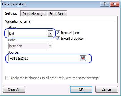
- Select List.
- Source: Select table headers.
- Press with left mouse button on OK button.
4.2 Create a named range
- Go to tab "Formulas".
- Press with left mouse button on "Name Manager" button.
- Press with left mouse button on "New.." button.
- Enter a name.
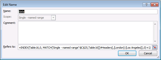
- Enter the following formula:
=INDEX(Table16,0, MATCH('Single - named range'!$C$25,Table16[[#Headers],[London]:[Los Angeles]],0)+1)
- Press with left mouse button on OK button.
4.3 Explaining the named range formula
Step 1 - Find column in Excel Table based on the selected drop-down list value
The MATCH function returns the relative position of an item in a cell range.
MATCH(lookup_value, lookup_array, [match_type])
The first argument lookup_value is the drop down list cell, the second argument is a cell reference to the Excel Table column header names, and the third argument is 0 (zero) which means there must be an exact match.
MATCH('Single - named range'!$C$25,Table16[[#Headers],[London]:[Los Angeles]],0)
becomes
MATCH("London",{"London","Tokyo","Los Angeles"},0)
and returns 1.
Step 2 - Return values from column
The INDEX function returns a single value or multiple values based on a row and optionally a column number.
INDEX(array, [row_num], [column_num])
The first argument is an array or a cell reference, in this case, a cell reference to Excel Table named Table16.
The second argument is the row number, however, if you use 0 (zero) the INDEx function returns all the value from the specified Excel Table column.
INDEX(Table16,0, MATCH('Single - named range'!$C$25,Table16[[#Headers],[London]:[Los Angeles]],0)+1)
becomes
INDEX(Table16,0, 1+1)
There is a column before the column name "London" in the Excel Table, that is why we need to add 1.
INDEX(Table16,0, 1+1)
becomes
INDEX(Table16,0, 1+1)
and returns {5; 5; 8; 9; 13; 16; 18; 18; 16; 12; 8; 6}.
4.4 Setting up the chart

Here are the steps to create the chart:
- Press with right mouse button on on chart.
- Press with left mouse button on "Select Data...".
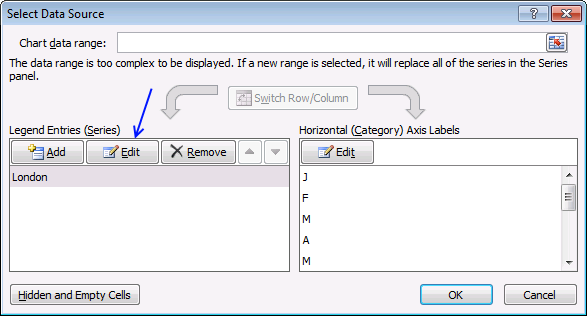
- Press with left mouse button on "Edit" button (Legend Entries).
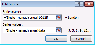
- Series name: Cell C25.
- Series values: The named range "data". Don't forget the worksheet name!
- Press with left mouse button on OK button.
- Press with left mouse button on OK button again.
5. "Helper" table
The following example has two tables and a drop-down list. The table to the right has "dynamic" values and they change depending on the chosen value in cell C25. But if you add values to the first table, the second table does not automatically include the new values. You have to change the table size yourself.
It is not as pretty as a named range but easier to work with if you want multiple data columns and chart series. The attached file below contains an example with multiple chart series.
5.1 Drop down list

- Select cell C25.
- Go to tab "Data" on the ribbon.
- Press with left mouse button on "Data Validation" button.
- Go to tab "Settings".
- Select List.
- Source: Select table headers.
- Press with left mouse button on OK button.
5.2 Create the second table

- Type month in cell F1 and city in cell G1.
- Select cell range F1:G13.
- Go to tab "Insert" on the ribbon.
- Press with left mouse button on "Table" button.
- Press with left mouse button on "My tables has headers".
- Press with left mouse button on OK.
5.3 Enter Excel Table formula

- Select cell F2.
- Type:
=Table1[@Month]
and press Enter.
- Select cell G2.
- Type:
=INDEX(Table1[@[London]:[Los Angeles]],MATCH($C$25,Table1[[#Headers],[London]:[Los Angeles]],0))
- Press Enter.
7. Change chart series by pressing on data - VBA

The image above shows a chart populated with data from an Excel defined Table. The worksheet contains event code that changes the shown cart series based on which cell is selected. See the animated image below.

You can also select multiple cells in the table by press and hold with the left mouse button and then drag with the mouse to select multiple cells.

If you want to select cells that are not adjacent you can press and CTRL key and then press with left mouse button on the cells you want to select. The corresponding chart series shows up in the chart automatically, this is made possible with event code.
VBA code
'Event code
Private Sub Worksheet_SelectionChange(ByVal Target As Range)

'Dimension variables and declare data types
Dim ACell As Range
Dim ActiveCellInTable As Boolean
Dim c As Single
Dim str As String

'Iterate every cell in selection
For Each ACell In Target

    'Enable error handling
    On Error Resume Next

    'If selected cell is in a table and the table name is Table1, save TRUE in ActiveCellInTable (boolean)
    ActiveCellInTable = (ACell.ListObject.Name = "Table1")

    'Resume normal error handling (stop if an error occurs)
    On Error GoTo 0

    If ActiveCellInTable = True Then

        'Save cell reference (First column in table) if str is empty
        If str = "" Then str = "Table1[[#ALL]," & ACell.ListObject.Range.Cells(1, 1).Value & "]"

        'Calculate selected cell's column number in table
        c = ACell.Column - ACell.ListObject.Range.Cells(1, 1).Column + 1

        'Check if column number is above 1
        If c > 1 Then

            'Add cell reference
            str = str & "," & "Table1[[#ALL]," & ACell.ListObject.Range.Cells(1, c).Value & "]"

            'Change "Chart 1" data source
            ChartObjects("Chart 1").Chart.SetSourceData Source:=Range(str)
        End If
    End If
Next ACell

End Sub
Where to put the code?

- Press Alt + F11 to open the Visual Basic Editor.
- Press with right mouse button on on sheet name Sheet1.
- Press with left mouse button on on "View Code".
- Copy/Paste VBA code to sheet module.
- Exit Visual Basic Editor and return to Excel.
8. Change chart data range using a Drop Down List - VBA

In this article I will demonstrate how to quickly change chart data range utilizing a combobox (drop-down list). The above image shows the drop-down list and the input range is cell range E2:E4.
Cell range E2:E4 contains the table names that points to Excel defined Tables located on sheet 2011, 2010 and 2009, see picture below. When you select a table name in the drop-down list, the chart is instantly populated and refreshed, see picture above.

Excel defined Tables are great to work with, they expand automatically when new values are added, this makes charts with data sources pointing to Excel defined Tables easy to work with. You don't need to adjust the cell references when records are added or deleted.
Here are the steps to set up this scenario:
Create a chart
- Go to "Insert" tab
- Press with left mouse button on "Column chart" button
- Press with left mouse button on "Clustered Column" chart button
Create Combo Box
- Go to "Developer" tab
- Press with left mouse button on "Insert controls" button
- Press with left mouse button on Combo Box (Form Control)
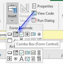
- Press with left mouse button on and drag on the worksheet to create the combobox.
Add VBA code to a module
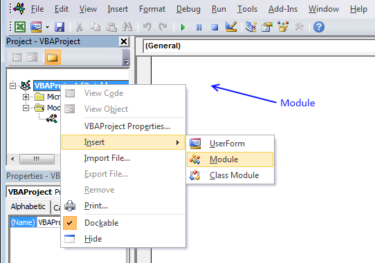
- Press Alt + F11 to open the VB Editor.
- Press with right mouse button on on your workbook in the Project Explorer window.
- Press with left mouse button on "Insert"
- Press with left mouse button on "Module" to insert a module to your workbook.
- Copy VBA code below (Ctrl + c)
- Paste VBA code to the code module, see image above.
- Return to Excel
VBA code
'Name macro
Sub SelectTable()

'Apply actions to selected drop-down list
With ActiveSheet.Shapes(Application.Caller).ControlFormat

    'Make sure the selected drop-down list name is "Drop Down 1"
    If ActiveSheet.Shapes(Application.Caller).Name = "Drop Down 1" Then

        'Change Chart 1 data source
        Worksheets("Chart").ChartObjects("Chart 1").Chart.SetSourceData Source:= _
        Range(.List(.Value) & "[#All]")
        Worksheets("Chart").ChartObjects("Chart 1").Chart.PlotBy = xlRows
    End If
End With

End Sub
Assign macro
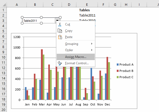
- Press with right mouse button on combo box.
- Press with left mouse button on "Assign macro...".
- Press with left mouse button on "SelectTable".
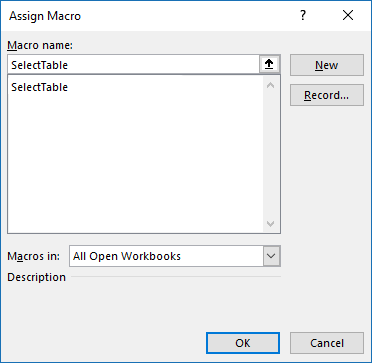
- Press with left mouse button on OK button.
Populate Combo Box
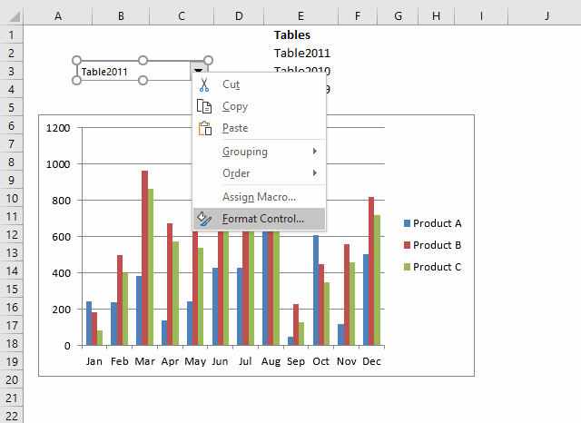
- Press with right mouse button on combo box.
- Press with left mouse button on "Format control..." and a dialog box appears, see image below.
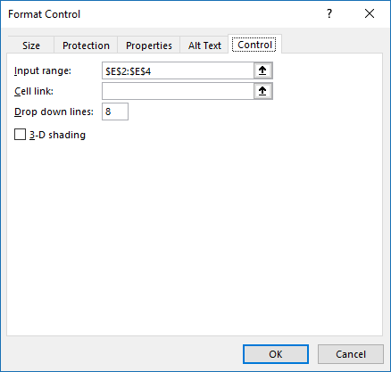
- Go to tab "Control".
- Press with left mouse button on "Input range" button.
- Select cell range E2:E4.
- Press with left mouse button on OK button.
Built-in Charts
Combo Charts
Combined stacked area and a clustered column chartCombined chart – Column and Line on secondary axis
Combined Column and Line chart
Chart elements
Chart basics
How to create a dynamic chartRearrange data source in order to create a dynamic chart
Use slicers to quickly filter chart data
Four ways to resize a chart
How to align chart with cell grid
Group chart categories
Excel charts tips and tricks
Custom charts
How to build an arrow chartAdvanced Excel Chart Techniques
How to graph an equation
Build a comparison table/chart
Heat map yearly calendar
Advanced Gantt Chart Template
Sparklines
Win/Loss Column LineHighlight chart elements
Highlight a column in a stacked column chart no vbaHighlight a group of chart bars
Highlight a data series in a line chart
Highlight a data series in a chart
Highlight a bar in a chart
Interactive charts
How to filter chart dataHover with mouse cursor to change stock in a candlestick chart
How to build an interactive map in Excel
Highlight group of values in an x y scatter chart programmatically
Use drop down lists and named ranges to filter chart values
How to use mouse hover on a worksheet [VBA]
How to create an interactive Excel chart [VBA]
Change chart series by clicking on data [VBA]
Change chart data range using a Drop Down List [VBA]
How to create a dynamic chart
Animate
Line chart Excel Bar Chart Excel chartAdvanced charts
Custom data labels in a chartHow to improve your Excel Chart
Label line chart series
How to position month and year between chart tick marks
How to add horizontal line to chart
Add pictures to a chart axis
How to color chart bars based on their values
Excel chart problem: Hard to read series values
Build a stock chart with two series
Change chart axis range programmatically
Change column/bar color in charts
Hide specific columns programmatically
Dynamic stock chart
How to replace columns with pictures in a column chart
Color chart columns based on cell color
Heat map using pictures
Dynamic Gantt charts
Stock charts
Build a stock chart with two seriesDynamic stock chart
Change chart axis range programmatically
How to create a stock chart
Excel categories
39 Responses to “How to filter chart data”
Leave a Reply
How to comment
How to add a formula to your comment
<code>Insert your formula here.</code>
Convert less than and larger than signs
Use html character entities instead of less than and larger than signs.
< becomes < and > becomes >
How to add VBA code to your comment
[vb 1="vbnet" language=","]
Put your VBA code here.
[/vb]
How to add a picture to your comment:
Upload picture to postimage.org or imgur
Paste image link to your comment.
How would I adapt this to work if I have a number of stacked series in the chart, each with a defined range? Each time I update the chart, I want it to pull data from the same sheet, same rows, just offset columns.
Amanda,
read this: Dynamic chart – Display values from a table row or column
How can I adapt the code to run on Excel 2003, I did in 2010 and works fine, but in 2003 had an error (Range error on method _Global)
Worksheets("Chart").ChartObjects("Chart 1").Chart.SetSourceData Source:= _Range(.List(.Value) & "[#All]")
Any clue?
Hernan Delgado,
Maybe this answers your question:
https://www.excelforum.com/excel-programming-vba-macros/386423-vba-error-unable-to-set-the-values-property-of-the-series-class.html
Hi,
When I insert the combobox at the end of the instructions, nothing is present in the drop down. I was wondering if you would be able to help with that?
Thanks for the help!
Ash
Ash,
I have added instructions, see above: Populate combo box
Amanda,
Thanks!
Hi Ash,
Select "Design Mode" on the Developer tab, then press with right mouse button on the combobox and select Properties. In the ListFillRange field enter the range of cells that hold the values you would like in the dropdown. Close the Properties window, deselect "Design Mode" and I believe you should be good to go.
I have tabular data that is dymanic how could i change this vba to update a charts range from this tabular data. needs to be vba as the number of series changes when the data changes,
Charles,
please explain in greater detail or preferably upload a workbook without sensitive data.
[...] I'm probably going to go with the following method, when I get my data organised that is!!..... Change chart data range using a drop down list (vba) | Get Digital Help - Microsoft Excel resource Cheers. [...]
Hi,
Happy to see above code but when i try to incorporate the above code in to excel its not working kinldly guide
Best Regards
Rahul jadhav
Rahul Jadhav,
What happens?
Hi Oscar,
Glad to see your reply.
i would like to tell you that I got your file and checked the macro and its working fine.
would like to say few words regarding this website, you have develope it very nicely. i am working on excel from last 7-8 years and i have never come across any website like this. good job done and its really very helpful to understand different Scenario.
good work and best wishes
Rahul Jadhav
India
Rahul Jadhav,
Thank you!
Hello Oscar,
Thanks for sharing the excel options
I am getting the error message, when i have more than 10 columns on selection
saying range of object worksheet failed
debbug shows in last line
Thanks
narayan
Narayan,
can you provide a workbook?
Upload here
It works like charm. I was just wondering if there is a way to get the vba set the source data in a dual axis environment. Setting the source data on primary axis from the drop down, while leave the secondary axis intact, with its setting, or have another drop down for it?
I can't get it to work. Can you provide more details about how to link up the combo box to the actual tables please? When I try to run a macros, it also gives me "Type Mismatch" error message
Thanks,
Yuri
Yuri,
Check the combo box name and that it matches the shape name in the vba code.
Hi There,
I am getting the following error.
Run-Time error'-2147352571(80020005)
The item with the specified name wasn't found for the below line code
With ActiveSheet.Shapes(Application.Caller).ControlFormat
Manish,
Your drop down list must be named "Drop Down 1"
or change the name here accordingly:
If ActiveSheet.Shapes(Application.Caller).Name = "Drop Down 1" Then
Your works are wonderful
Hi,
Found this thread and I am hoping it is still active.
Two Questions:
1. I have four items that need to be in my drop down box, instead of three. How would you go about adding a 2012 table to the spreadsheet and enable the macro to recognize the new sheet? When I tired I got an error message even though all I did was copy one of the existing sheets and renamed it.
2. Is there a way that I can rename the sheets using a word rather than a number? For instance, instead of the current name of the sheets (2009,2010,2011), I would like to use the words Gender, Race, etc. Again, I got an error message when I attempted to do this. In fact, I got the same error message in both cases.
Jeff Lucas,
1. I have four items that need to be in my drop down box, instead of three. How would you go about adding a 2012 table to the spreadsheet and enable the macro to recognize the new sheet? When I tired I got an error message even though all I did was copy one of the existing sheets and renamed it.
Add a new table and name the table, not the sheet, Table2012.
2. Is there a way that I can rename the sheets using a word rather than a number? For instance, instead of the current name of the sheets (2009,2010,2011), I would like to use the words Gender, Race, etc. Again, I got an error message when I attempted to do this. In fact, I got the same error message in both cases.
You can name the tables or sheets whatever you want, almost.
Get the following Excel example file, it has a fourth table named Table2012 and it is on sheet2.
change-chart-data-rangev2.xlsm
Thank you so much! This worked perfectly!
Is there a way to use this method with pivot tables? I'm having some difficulty updating the structured references of the normal tables to those of pivot tables.
Hi Oscar, thanks for this amazing article - especially for updating with more basic how to create a drop-down menu it makes it so much more accessible.
I wanted to know, can this work where your tables are BETWEEN workbooks? Like, you have one Excel file for 2014, one for 2013, etc.
Many thanks.
Dear Sir,
I was trying to figure out how this code actually works, as since I am very new to VBA coding I was not able to understand why the code always makes its own chart even if you provide your axis series.
My data is in the reverse form as in North East West South are in column not in rows.
Hope you would help.
Hi,
Can you tell me what if i want to change the data of chart and use this code to make the similar chart and can i also copy and paste it in my final presentation without showing the background work just chart with drop down
Hi,
I need exactly same thing. BUT instead of Tables, i have Pivot Tables, Which i want to switch as data Source for a Chart. Can you give the Macro for that?
Great Work Sir!
Gagan Brar,
A pivot chart or a regular chart?
tancks
Hi,
I have tried to populate a chart with values selected from drop down combo box list. My challenge here is it has populate from different column and row based on the value selected in the dropdown list. the cells will be constant like E and F column will only be selected for the chart but it might take from E1-23 or E 24-E30 or E30 - E40 depending on the value selected from combo box. combo box will have headers like for example server name, so based on the server name displayed the chart has to change by picking up values from E and F columns either E1-24 or E24-30 or E3-0-40,F1-24 or F24-30 or F3-0-40. I want this to be done automatically using VBA.
My Present Code:
Sub create_chart_sheet()
Dim oChartObj As ChartObject
Application.ScreenUpdating = False
Application.Calculation = xlCalculationManual
Set oChartObj = ActiveSheet.ChartObjects.Add(Top:=0, Left:=0, Width:=50, Height:=50)
'Add Data to Chart Sheet
oChartObj.Chart.SetSourceData Sheets("log").Range("A2:F69")
Set oChartObj = ActiveSheet.ChartObjects.Add(Top:=60, Left:=400, Width:=450, Height:=450)
With oChartObj.Chart
'.ChartType = xlPie
.ChartType = xlBarClustered
.SeriesCollection.NewSeries
.SeriesCollection(1).Name = "Server Disk Usage"
.SeriesCollection(1).XValues = ActiveSheet.Range("F3:F23") ' Hardcoded for one server
.SeriesCollection(1).Values = ActiveSheet.Range("E3:E23")
Dim oChart As Chart
Set oChart = Sheets("log").ChartObjects(1).Chart
'Set oChartObj = Charts("log")
oChart.HasTitle = True
oChart.ChartTitle.Text = "Server Disk Usage"
End With
Application.ScreenUpdating = True
Application.Calculation = xlCalculationAutomatic
End Sub
If you want to change the row instead of the column, what will the VBA code be?
MAHMOUD,
It is not possible to reference a row in an Excel Table using structured references, at least no with my approach.
I recommend that you copy and with "Paste Special..." transpose the Excel table so the rows become columns and columns become rows.
You also need to create an Excel Table with the new values before trying the macro again.
MAHMOUD
Here is an image.
I also renamed the Table1 to Table2 and the new Table to Table1.
I NEED MAKE CHART BY MONTH NOT BY NORTH OR SOUTH
Hi,
I tried the method- Use a named range to change chart data
In my case I am also using some slicers on the data. It worked perfectly. But when I save and close the file, and then reopen again -- the "series values" of the chart changes from 'sheet_name!data' to 'file_name!data'. Due to this when selecting a different value in the slicer, the data in the table changes but not in the chart, the chart remains constant no matter what i select in the slicer.
I am trying to understand where this code is coming from. I'm tasked with creating a table that has 38 categories(like your months) and 12 instances(like your directions except mine is months). I need to be able to press with left mouse button in the column for each month to display that month's data for each category. I have it oriented so my months are across the top of the table and my categories are down the left side but it doesn't work. It gives a chart with random numbers down the left axis and that's it. I was looking at your code in the module1 where you set your source range and I was confused about where the A11:A17 and D11:D17 came from since that's not the expanse of your source data. If you could break down what I would need to know to make this applicable for me I would greatly appreciate it.