How to add horizontal line to chart
This tutorial shows you how to add a horizontal/vertical line to a chart. Excel allows you to combine two types of charts, in this case, I am going to combine the column and the x y scatter chart.
What's on this page
1. Introduction
Why would you want to use a horizontal line?
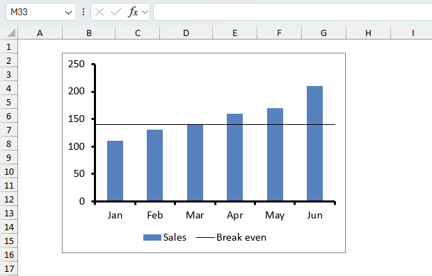
It could be a break-even line for revenue or a threshold making it easy to spot specific dates/months/years containing interesting data points.
There are, of course, many more applications. I am also going to demonstrate how to insert a vertical line into a bar chart. Check out the Charts category for more interesting articles.
Why use a vertical line?
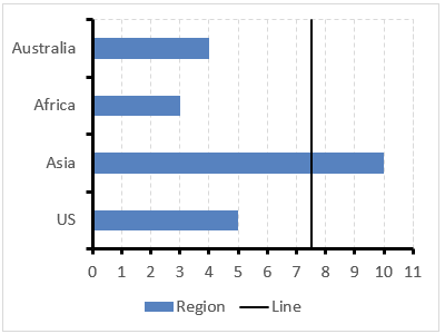
A vertical line on a bar chart would be just as useful as a horizontal line on a column chart.
Why use a advancing or declining line?
The custom line could be a trend-line showing the average gain across a time interval. A trend-line in an Excel chart is useful in several situations where you need to analyze data patterns and make predictions.
- Sales and Revenue Forecasting
- Stock Market Analysis
- Quality Control in Manufacturing
and much more. Excel has a built-in trend line tool if you don't want to create a custom line.
2. How to add a horizontal line
2.1 Insert a chart
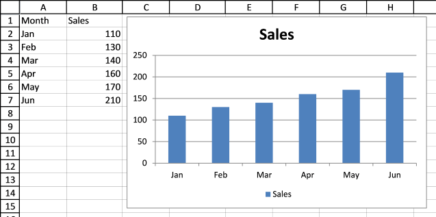
The first step is to create a chart with only one series. You can see my data in cell range A1:B7, see picture below.
- Select cell range A1:B7.
- Go to tab "Insert" on the ribbon.
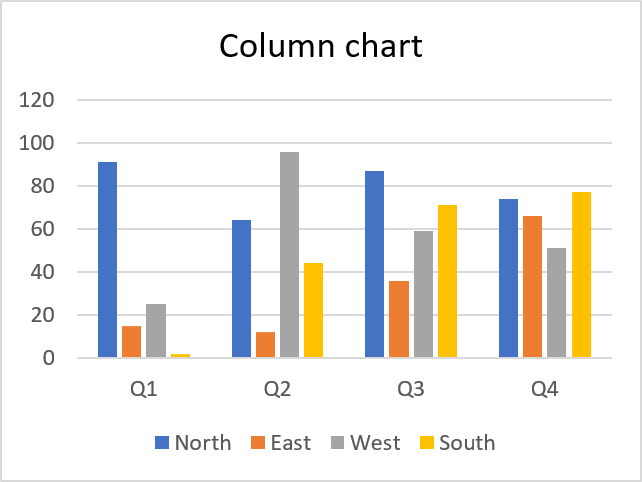
- Press with left mouse button on the "Column chart" button.
The Excel column chart is created, shown in the picture below.
2.2 Add a second series
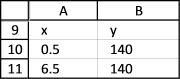
Now it is time to build the line. I will now add more data, see cell range A9:B11 in the picture below.
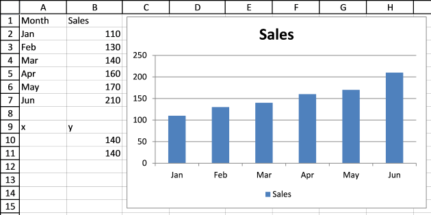
This series will be the horizontal line on the y-axis value 140.
- Press with right mouse button on on the chart.
- Press with mouse on "Select Data...".
- Press with left mouse button on "Add" button.
- Select cell B9 for "Series name:".
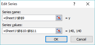
- Select cell range B10:B11 for series values.
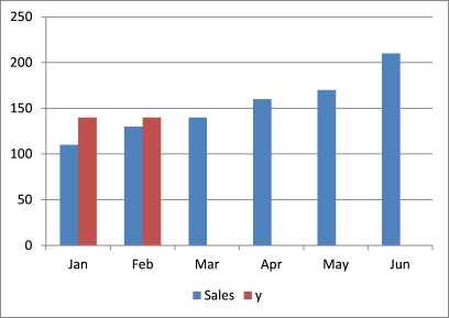
Excel colored the second series differently so you can distinguish them easily. There are only two columns in the second series because of the two cells we selected as series values.
Related article:
Recommended articles

What's on this page Custom data labels Improve your X Y Scatter Chart with custom data labels How to apply custom […]
2.3 Change series chart type
I am now going to change the chart type for the second series.
- Press with right mouse button on on the second series on the chart.
- Press with mouse on "Change Series Chart Type".
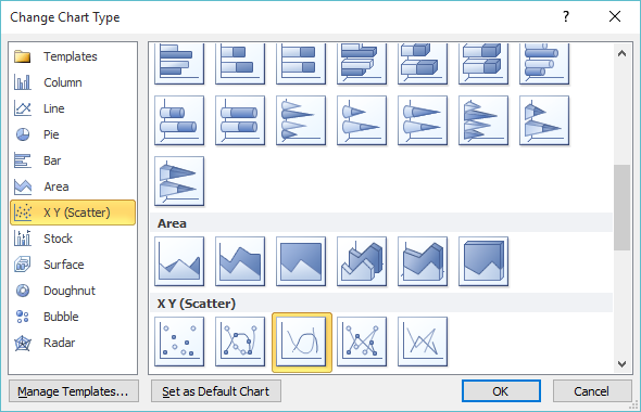
- Select chart type "Scatter with smooth lines".
- Press with left mouse button on OK button.
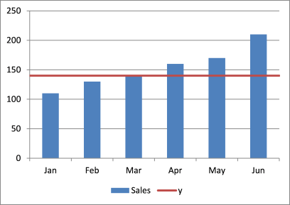
The second series is now a red line between Jan and Feb.
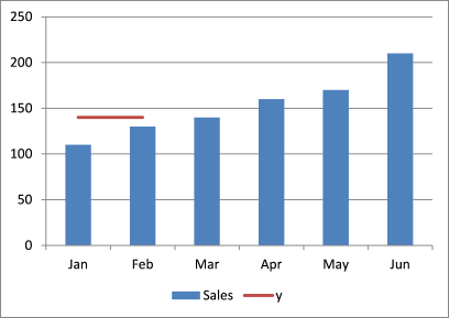
You can change the width and angle of the line by editing the values in cell range A10:B11.
Related post:
Recommended articles
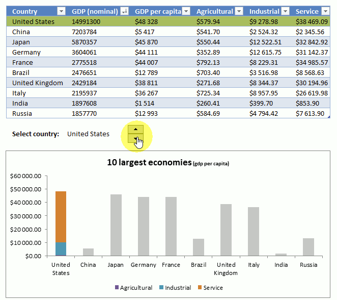
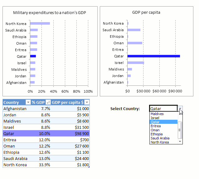
This interactive chart allows you to select a country by press with left mouse button oning on a spin button. […]
2.4 Build a horizontal line
- Type 0.5 in cell A10.
- Type 6.5 in cell A11.
- Press with right mouse button on on chart.
- Press with mouse on "Select Data...".
- Select series "y".
- Press with mouse on "Edit" button.
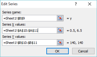
- Select cell range A10:A11 for "Series X values:".
- Press with left mouse button on OK.
- Press with left mouse button on OK.
Related post:
Recommended articles
This article demonstrates how to highlight a bar in a chart, it allows you to quickly bring attention to a […]
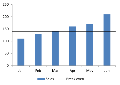
2.5 Final chart customizations
These are the steps I made to remove grid lines, create a smaller line and change the second series name value.
- Press with mouse on a grid line.
- Press the Delete button on the keyboard.
- Double press with left mouse button on a horizontal line.
- Decrease line width.
- Change line color.
- Press with left mouse button on Close button.
- Type "Break even" in cell B9.
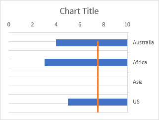
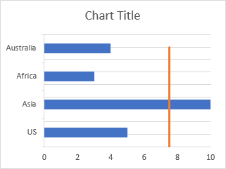
3. How to add a vertical line to a chart
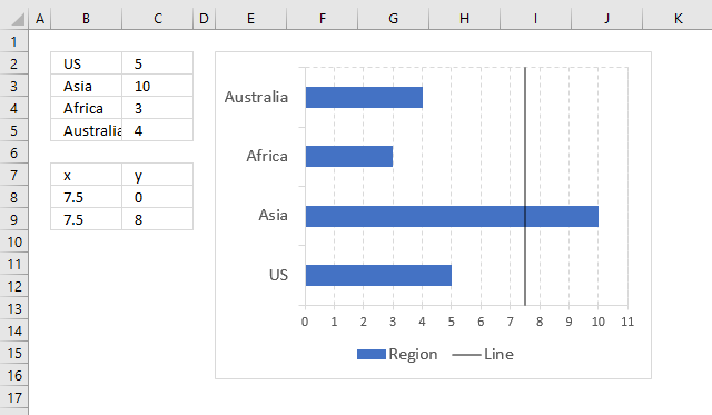
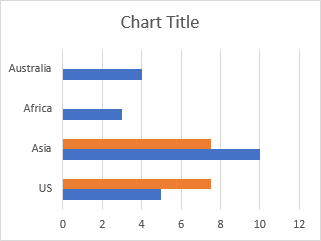
A vertical line on a bar chart would be just as useful as a horizontal line on a column chart.
The picture above shows a black line on value 7.5 with transparency ca 50%.
Here is how I built this chart.
3.1 Insert a bar chart
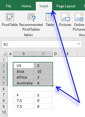
- Select the data.
- Press with mouse on "Insert" on the ribbon.
- Press with mouse on "Column" chart button.
- Press with left mouse button on "2D Clustered Bar"
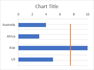
The bar chart is now visible next to the data.
3.2 Add a second series
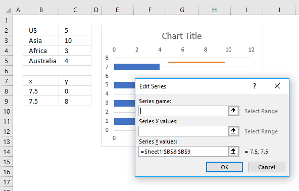
The x value is where on the chart I want the line to appear, the y value is a value you probably have to guess and adjust later.
- Press with right mouse button on on the chart and press with left mouse button on "Select Data..."
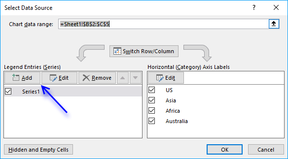
- Press with mouse on "Add" button shown above.
- Select the x values.
- Press with left mouse button on OK button.
- Press with left mouse button on OK button.
The chart now contains two series, the first series is blue and the second series is red.
3.3 Change the chart type of the second series
- Press with right mouse button on on the chart and then press with left mouse button on "Change Chart Type...".
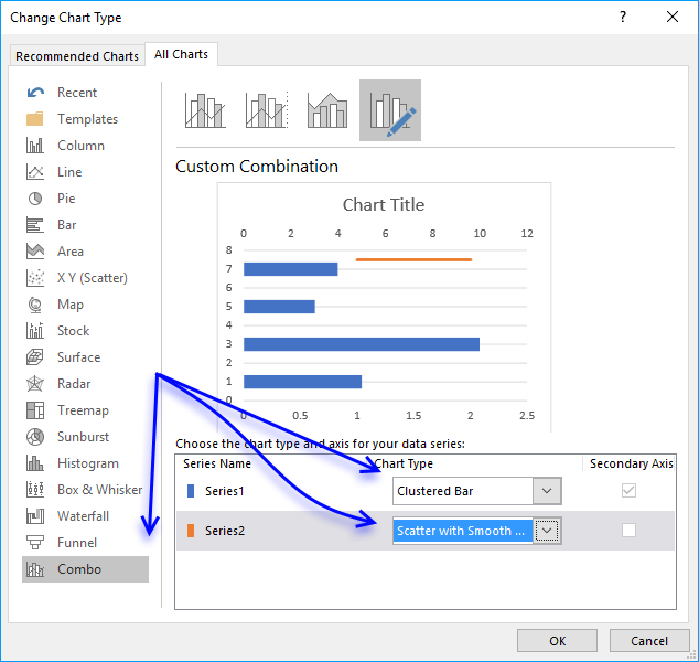
- Press with mouse on tab "Combo"
- Select the clustered bar chart for series1.
- Select the Scatter with smooth lines chart for series2.
- Press with left mouse button on OK button.
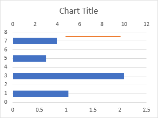
The chart above has two x axis, one at the top and one at the bottom. The y axis regions disappeared and new y axis values appeared.
We certainly have some cleaning up to do.
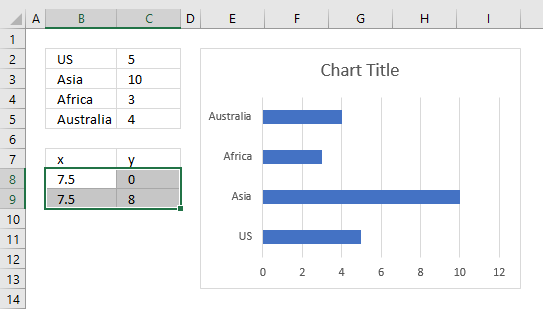
3.4 Adjust scatter chart values
- Press with right mouse button on somewhere on the chart.
- Press with left mouse button on on "Select Data...".
- Select Series2.
- Press with mouse on "Edit" button.
- Select the x values.
- Select the y values.
- Press with left mouse button on OK button.
- Press with left mouse button on OK button.
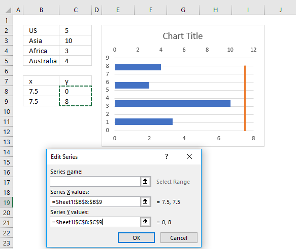
The chart now looks like this.
3.5 Chart formatting
- Delete all axis values
- Select the chart.
- Go to tab "Design" on the ribbon.
- Press with left mouse button on "Add Chart Element" button.
- Press with left mouse button on "Axis".
- Press with left mouse button on "Secondary Horizontal ".
- Repeat steps 4-5, then add a "Vertical Horizontal" axis.
To move the axis region values left follow these steps.
- Double press with left mouse button on the x axis values above plot area.
- Go to tab "Axis Options"
- Select "Vertical Axis crosses" axis value 0 (zero).
To move the axis values follow these steps.
- Double press with left mouse button on the y axis values to the left of the plot area.
- Go to tab "Axis Options"
- Select "Horizontal axis crosses" at category number: 0 (zero).
- Exit Settings
Double press with left mouse button on the line to open the settings. Change the line color, width and transparency.
The line is not covering the entire plot area, here is how to fix that.
- Select the chart.
- Go to tab "Design"
- Add the "Primary Vertical" axis
- Double press with left mouse button on axis values to open the settings.
- Go to tab "Axis Options"
- Change the maximum value so that the line covers the entire plot area. 8 worked for me.
- Delete the "Primary Vertical" axis.
To add a Legend follow these steps.
- Select chart.
- Go to tab "Design" on the ribbon, it appears when you select a chart.
- Press with left mouse button on the "Add Chart Element" button.
- Press with left mouse button on "Legend".
- Pick a position for the "Legend".
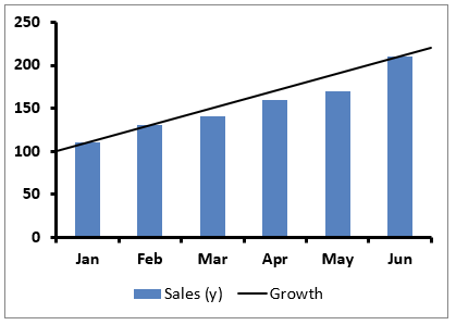
4. Create a straight line through the first and last chart column

The image above demonstrates a custom chart line that fits the first and last column only.
4.1 Calculate the slope between the first and last column

We want a line that begins at the first column and ends with last column. We can use the SLOPE function to calculate the slope of this line.
Formula in cell C16:
=SLOPE(C10:C11, B10:B11)
The SLOPE function needs at least two coordinates (x, y) to calculate the slope, the first coordinate is (1,110) and the second coordinate is (6,210).
Type the x-coordinate of the first coordinate in cell B10 and the y-coordinate in cell C10, repeat with the second coordinate in cells B10:B11. We need these values to create the custom line.
4.2 Create a line on the chart
- Press with right mouse button on on the chart.
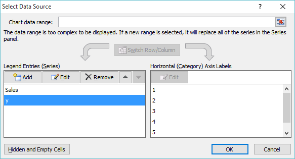
- Press with mouse on "Select Data...". A dialog box appears.

- Press with mouse on "Add" button. Another dialog box appears.

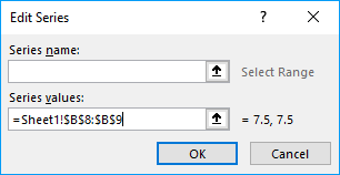
- Press with mouse on the button next to field "Series values:", select cell range C10:C11.
- Press with left mouse button on the OK button, see the image above. You are now back to the first dialog box.
- Press with left mouse button on the OK button on the first dialog box to apply changes.

The chart above shows the second series we just created, however, we want it to be a line not another series of columns. Here is how to change the chart type:
- Press with right mouse button on on the chart.
- Press with mouse on "Change Chart Type...".

- A dialog box appears. Press with mouse on "Combo chart".

- Select Chart Type: "Scatter with Straight..." for Series2.
- Press with left mouse button on check box "secondary Axis".
- Press with left mouse button on OK button.

There is now a line displayed on the chart, if we change the x-axis values for this line we get a line that fits both the first and last column.
- Press with right mouse button on on the chart.
- Press with mouse on "Select data...". A dialog box appears.

- Press with mouse on Series2 to select it, see image above.
- Press with mouse on the "Edit" button to change x-axis values. Another smaller dialog box is now visible, see the image below.

- Press with mouse on the arrow button next to the "Series X values:" field, see the image above.
- Select cell range B10:B11.
- Press with left mouse button on the "OK" button. You are now back to the first dialog box.

- Press with left mouse button on the "OK" button to apply changes.

The line now fits both the first and last column, here is how to extend the line to both y-axis borders.
We calculated the slope of the line in cell C16, we can now use that value to extend the line to both sides.
Change x value in cell B10 to 0.5 and subtract 110 with 20/2 equals 100. Change the x value in cell B11 to 6.5 and change the value in cell C11 to 220 (210+20/2).

Charts category
Table of Contents How to add lines between stacked columns/bars (Excel charts) Use slicers to quickly filter chart data How […]
Table of Contents How to create an interactive Excel chart How to filter chart data How to build an interactive […]
Table of Contents How to graph a normal distribution How to build an arrow chart How to graph an equation […]
Column chart category
This article demonstrates how to create a chart that animates the columns when filtering chart data. The columns change incrementally […]
What is on this page? Built-in charts How to create a column chart How to create a stacked column chart […]
Scatter x y chart category
Table of Contents How to graph a normal distribution How to build an arrow chart How to graph an equation […]
What's on this page Custom data labels Improve your X Y Scatter Chart with custom data labels How to apply custom […]
Excel categories
One Response to “How to add horizontal line to chart”
Leave a Reply
How to comment
How to add a formula to your comment
<code>Insert your formula here.</code>
Convert less than and larger than signs
Use html character entities instead of less than and larger than signs.
< becomes < and > becomes >
How to add VBA code to your comment
[vb 1="vbnet" language=","]
Put your VBA code here.
[/vb]
How to add a picture to your comment:
Upload picture to postimage.org or imgur
Paste image link to your comment.
Hello Oscar Cronquist,
“How to add horizontal line to chart”
Thank You SO MUCH for the tutorial that you provided!!!
I’ve been trying to do this for about 20 hours.
I’ve looked online and have watched MANY tutorials.
None of the tutorials allowed me to “Add horizontal line to chart” until I tried your tutorial.
Your tutorial is to the point and easy to follow.
Thank You!
Best Regards,
Jeff Goodson