How to animate an Excel chart

This article demonstrates how to create a chart that animates the columns when filtering chart data. The columns change incrementally between values which gives it a smoother appearance.
The drop-down list lets the Excel user select an item. An event macro checks if there is a new drop-down list value. It then compares old and new series values so it can calculate new values, in small steps.
What's on this page
1. Introduction
What is an Excel Chart?
An Excel chart is a visual representation of data from a spreadsheet. It transforms values into graphical objects like lines, bars, etc.. , making it easier to identify trends, patterns, and comparisons.
What is a line chart?
A line chart displays data points connected by lines. It’s useful for showing trends over time. It allows you to easily see the progression or changes in your data set.
What is a bar chart?
A bar chart uses rectangular horizontal bars to represent data values. Each bar’s length is proportional to the value it represents. Bar charts are great for comparing discrete or categorical data making differences easy to spot.
What is a column chart?
A column chart contains vertical bars that displays data points. The height corresponds to the value it represents. The difference between bar and column charts is the way the bars are oriented, horizontal or vertical.
Why animate charts?
Animating charts brings your data to life in several ways. Dynamic visuals capture attention better than static images. Step-by-step animations can guide viewers through more complex data. It makes it easier to understand how values change over time. Animations can highlight key data points or trends. It makes sure the audience focuses on the most important information.
What is VBA?
VBA (Visual Basic for Applications) is a programming language developed by Microsoft that is used for automating tasks in Microsoft Office applications such as Excel, Word, and Access. It allows users to create macros, automate repetitive tasks, and enhance Office functionality with custom scripts.
What is a macro?
In Microsoft Excel, a macro is a sequence of instructions written in Visual Basic for Applications (VBA) that allows you to automate repetitive tasks time consuming tedious tasks. Macros can perform a wide range of actions from simple formatting changes to complex data manipulations.
What is an event?
An event in Excel refers to an action or occurrence that triggers the execution of a specific macro. Events can be user-initiated, such as opening a workbook, changing a cell's value, or press with left mouse button oning a button, or system-initiated, like recalculating a worksheet. By associating macros with events users can automate responses to specific actions within the workbook.
What is event code?
Event code is placed in specific object modules like ThisWorkbook or a worksheet module (Sheet1, Sheet2). Regular VBA code is typically stored in a standard VBA module like Module1, Module2, etc...
What is an *.xlsm file?
Older Excel versions saved Excel files using the *.xls as the file extension. It was also possible to save VBA code in an *.xls file which made them potentially unsafe.
Excel 2007 introduced *.xlsx and *.xlsm files which made it safer to use Excel files. An *.xlsx file cant contain VBA code at all making them safer to use in contrast to older *.xls files
An .xlsm file is a type of Excel workbook that also supports macros which are automated scripts written in VBA which *.xlsx don't do. They use the Open XML format and differ from standard .xlsx files because they can store and run macros. This feature extends the capabilities of worksheets allowing you to automate processes and improve spreadsheet functionality. It's important to exercise caution when handling .xlsm files from untrusted sources as macros can contain code that may pose security risks.
1. How to animate an Excel chart
 The image above demonstrates an animated column chart. It allows the user to interact with the chart by selecting regions on a drop-down list. Here is how it works:
- Drop-down list. The user selects a region by pressing the drop-down list button next to cell C12.
- Event code. An event macro changes the source data incrementally until the new values are present.
- Animate chart. The changes made by the event code animates the Excel chart.
1.1 Build a drop-down list
What is a drop-down list?
A drop-down list allows the Excel user to pick a value from a predefined list. It works like this:
- Press with left mouse button on with the left mouse button on the arrow next to the cell, see the animated image above.
- The drop-down list expands and shows items in a list.
- Press with mouse on one of the values to select it.
This allows you to control which values the Excel user can enter. An error message appears if an invalid value is entered. The drop-down list is one of many tools you can use to validate data, however, there is a couple of things you need to know about the regular drop-down list:
- It can easily be overwritten, simply copy another cell and paste it on a cell that contains a drop-down list and it is gone.
- You can't easily spot regular drop-down lists, you need to select the cell that contains a drop-down list to see it. I recommend that you format the cell to make it easier to find the drop-down list.
Here are the steps to create a drop-down list:
- Select cell C12.
- Go to tab "Data" on the ribbon.
- Press with mouse on "Data Validation button.
- Select tab "Settings".
- Select "List" in the drop down list "Allow:".
- Type North, East, South, West in Source field.
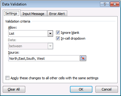
- Press with left mouse button on OK button.
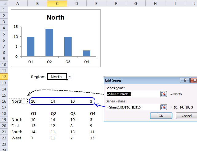
1.2 Formula

The formula in cell A16 verifies that the selected value in cell C12 exists in cell range A19:A22.
- The value in cell A16 is then used as the title in the column chart.
- Values in cells A16:E16 changes based on the selected value in cell C12.
- The chart uses cells B16:E16 to populate the chart.
Formula in cell A16
1.3 Explaining formula in cell A16

I recommend using the "Evaluate Formula" tool to troubleshoot and understand Excel formulas. Press with left mouse button on the cell you want to debug.
Go to tab "Formulas" on the ribbon. Press with left mouse button on the "Evaluate Formula" button located on the ribbon. A dialog box appears, see image above.
The Evaluate Formula tool lets you see the formula calculations in smaller steps, simply press with left mouse button on the "Evaluate" button to move to the next step.
The underlined expression is what is to be evaluated and the italicized expression is the most recent evaluated result. Press with left mouse button on the Close button to dismiss the dialog box.
Step 1 - Find relative position
The MATCH function returns a number representing the position of a given value in a cell range.
MATCH(C12,A19:A22,0)
becomes
MATCH("South",A19:A22,0)
becomes
MATCH("South",{"North";"East";"South";"West"},0)
and returns 3. "Item "South" is the third value in cell range A19:A22.
Step 2 - Return value
The INDEX function returns a value from a cell range based on a row and column number, the column number is optional.
INDEX(A19:A22,MATCH(C12,A19:A22,0))
becomes
INDEX(A19:A22, 3)
becomes
INDEX({"North";"East";"South";"West"}, 3)
and returns "South".
1.4 Insert column chart

- Select cell range A16:E16.
- Go to tab "Insert" on the ribbon.
- Press with mouse on the "Column charts" button.

- A pop-up menu appears, press with left mouse button on the "Clustered column" button. See image above.
- Create a column chart
1.5 Setting up the chart
- Press with right mouse button on on column chart, a popup menu appears.
- Press with mouse on "Select Data...".
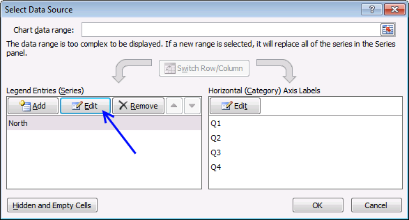
- Press with mouse on "Edit" button.
- Change series name to A16 and series values to B16:E16 (See picture below)
- Press with left mouse button on the OK button.
- Press with left mouse button on the OK button again.
1.6 Event Code
The event code calculates the steps needed to to make the chart animated, it returns new values, step by step, in cell range B16:E16 until they match the selected item's values.
'Event code
Private Sub Worksheet_Change(ByVal Target As Range)

'Dimension variables and declare data types
Dim i As Single, j As Single, x As Integer

'Check if changed cell is C12
If Target.Address = "$C$12" Then

    'Save cell values in cell range B16:E16 to variable cht
    cht = Range("B16:E16").Value

    'Enable error handling
    On Error Resume Next

        'Calculate relative position of value in cell C12 in cell range A19:A22 and save to variable x
        x = WorksheetFunction.Match(Range("C12"), Range("A19:A22"), 0) - 1

        'Ftop event code if an error has occurred
        If Err > 0 Then Exit Sub

    'Disable error handling
    On Error GoTo 0

    'Save new values to variable Nval based on variable x
    Nval = Range(Cells(19 + x, "B"), Cells(19 + x, "E")).Value

    'Iterate four times line between for and next
    For i = 1 To 4

        'Calculate incremental value
        Nval(1, i) = (Nval(1, i) - cht(1, i)) / 10
    Next i

    'Iterate ten times lines between for and next
    For i = 1 To 10

        'Iterate four times line between for and next, this is a nested for next statement
        For j = 1 To 4

            'Add incremental value array variable cht
            cht(1, j) = cht(1, j) + Nval(1, j)
        Next j

        'Save values in array variable cht to cell range B16:E16
        Range("B16:E16") = cht

        'Update worksheet
        DoEvents

        'A second DoEvents is required if you are using Excel 365
        DoEvents
    Next i
End If
End Sub
1.7 Where to put the code?

- Press with right mouse button on on the worksheet tab, a pop-up menu appears.

- Press with left mouse button on "View code", this opens the Visual Basic Editor and takes you to the worksheet module.
- Copy VBA code above.
- Press with left mouse button on in the code window.
- Paste code to window, see the second image above.
Recommended reading
Animation, Interaction and Dynamic Excel Charts
2. How to animate a line chart

This section demonstrates how to create an animation using a line chart in Excel. The user selects a series in a drop-down box and a macro animates the chart.
The animated image below shows what happens when the user selects a series, as you can see the chart has a small trailing shadow effect.
2.1 How I made this chart
The chart data is in cell range B3:J8. A small VBA macro calculates the difference between the current series and the new series and then divides it by 20. The result is shown in cell range C10:J10.
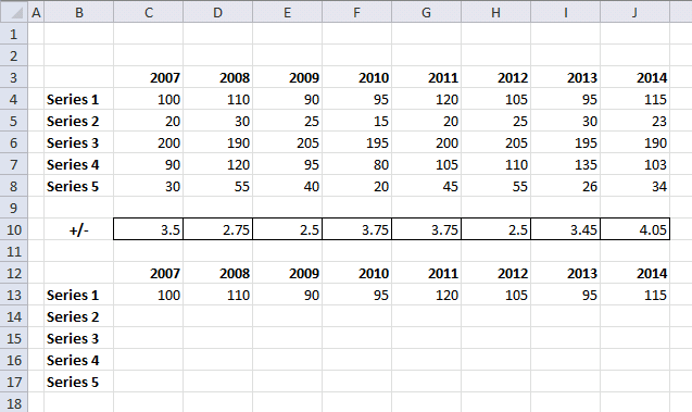
The chart data source is cell range C13:J17. The chart uses 4 lines to create the trailing shadow effect. Series 1 is the main line, the others are shadows.
Here you can see the calculations in action.
2.2 Event code
'Event code that fires as soon as any cell value in the worksheet has changed
Private Sub Worksheet_Change(ByVal Target As Range)

'If ... then statement - Check if target cell adress is equal to L6
If Target.Address = "$L$6" Then

    'Enable error handling
    On Error Resume Next

        'Find position of value saved cell L6 in cell range B4:B8 and save to variable x
        x = WorksheetFunction.Match(Range("L6"), Range("B4:B8"), 0) - 1

        'Stop macro if an error has occurred
        If Err > 0 Then Exit Sub

    'Disable error handling
    On Error GoTo 0

    'For ... Next statement- Iterate from 1 to 8 using variable i
    For i = 1 To 8

        'Calculate and save value from data table to cell range C13:J13
        Range("C10:J10").Cells(i) = (Range(Cells(4 + x, "C"), Cells(4 + x, "J")).Cells(i) - _
        Range("C13:J13").Cells(i)) / 20
    Next i

    'For ... Next statement- Iterate from 1 to 20 using variable i
    For i = 1 To 20

        'Save values in cell range C13:J16 to cell range C14:J17
        Range("C14:J17") = Range("C13:J16").Value

        'For ... Next statement- Iterate from 1 to 8 using variable j
        For j = 1 To 8

            'Add cell value from cell range C13:J13 and C10:J10 and save to cell range C13:J13 based on variable j
            Range("C13:J13").Cells(j) = Range("C13:J13").Cells(j) + Range("C10:J10").Cells(j)
        Next j

        'Show changes on screen
        DoEvents

        'And once again to make it work in Excel 365
        DoEvents
    Next i
    For j = 1 To 4
        Range("C14:J17") = Range("C13:J16").Value
        Range("C14:J14") = ""
        DoEvents
    Next j
End If
End Sub
2.3 Where to put the code?

- Righ-press with left mouse button on the worksheet tab located on the bottom left corner, see image above. A pop-up menu appears.
- Press with mouse on "View Code".
- The Visual Basic Editor opens up with the corresponding worksheet module open.

- Copy VBA code above.
- Paste VBA code to the worksheet module.
- Return to Excel.
Recommended articles
3. How to animate an Excel Bar Chart

This article demonstrates macros that animate bars in a chart bar. The image above shows a bar chart that animates one bar at a time, the bar grows until it reaches the correct value.
The "Clear chart" button clears all values in the chart. The "Animate" button starts the animation.
3.1 Slower animation (Previous Excel versions)
The animated image above shows a bar chart animation that has bars that grow more slowly. Press with left mouse button on the "Clear chart" button located to the right of the chart to delete the chart bars.
Press with left mouse button on the "Animate" button located below the "Clear chart" button to start the animation. The "Animate" button has a macro assigned named ClearChart displayed below.
3.2 VBA Code
'Name macro
Sub ClearChart()

'Delete values in cell range F3:F13
Range("F3:F13") = ""
End Sub
'Name macro
Sub Animate()

'Dimension variables and declare data types
Dim i As Single, j As Integer, k As Single

'For - next statement, count backwards from 11 to 1 using variable j
For j = 11 To 1 Step -1

    'Save value from cell range C3:C13 to variable k based on variable j
     k = Range("C3:C13").Cells(j).Value

         'For - next statement, count from 40 to number stored in variable k using variable i
         For i = 40 To k
            'Save value in variable i to cell in cell range F3:F13 based on number stored in variable j
            Range("F3:F13").Cells(j) = i

            'show changes on screen
            DoEvents
          Next i
Next j
End Sub
3.3 Where to put the VBA code?

You must copy the VBA code and paste it in a module in your workbook before you can use the macros.
- Copy the VBA code above or below on this webpage.
- Press Alt + F11 to open the Visual Basic Editor.
- Press with mouse on the "Insert" on the top menu, see image above.
- Press with mouse on "Module" to create a module. A module appears in the "Project Explorer" window. This is also shown in the image above.
- Paste the VBA code to the code module.
- Go back to Excel.
3.4 Explaining the chart animation
The bar chart's data source is cell range E2:F13. The macro begins with cell F13 and starts with value 40.
Then it adds 1 to 40, up to the value in C13 (45). The next cell is F12, starts at 40 and goes up to 50, one by one, and so on. See the picture below. The chart shows these changes in the data source as an animation.
3.5 Slower animation (Excel 365 subscription)
'Name macro
Sub ClearChart()

'Delete values in cell range F3:F13
Range("F3:F13") = ""
End Sub
'Name macro
Sub Animate()

'Dimension variables and declare data types
Dim i As Single, j As Integer, k As Single

'For - next statement, count backwards from 11 to 1 using variable j
For j = 11 To 1 Step -1

    'Save value from cell range C3:C13 to variable k based on variable j
     k = Range("C3:C13").Cells(j).Value

         'For - next statement, count from 40 to number stored in variable k using variable i
         For i = 40 To k
            'Save value in variable i to cell in cell range F3:F13 based on number stored in variable j
            Range("F3:F13").Cells(j) = i

            'show changes on screen
            DoEvents

            'Repeat to make it work in Excel 365
          Next i
Next j
End Sub
3.6 A faster animation (Previous Excel versions)
The animated image above shows a much faster bar chart animation.
3.6.1 VBA Code
Sub ClearChart()
Range("F3:F13") = ""
End Sub
'Name macro
Sub Animatev2()

'Dimension variables and declare data types
Dim i As Single, j As Integer, k As Single, s As Single

'For ... Next statement. Go from 11 to 1 using variable j
For j = 11 To 1 Step -1

    'Save value from cell in cell range C3:C13 to variable k based on variable j
    k = Range("C3:C13").Cells(j).Value

    'This line makes the animation faster, it calculates how fast the jump between numbers will be
    s = (k - 40) / 10

    'For ... Next statement. Go from 40 to number saved in variable k using variable i and s
    For i = 40 To k Step s

        'Save rounded number saved in variable i to cell in cell range F3:F13 based on variable j
        Range("F3:F13").Cells(j) = Round(i, 0)

        'Show changes on screen
        DoEvents
    Next i
Next j
End Sub
3.7 Faster animation (Excel 365 subscription)
Sub ClearChart()
Range("F3:F13") = ""
End Sub
'Name macro
Sub Animatev2()

'Dimension variables and declare data types
Dim i As Single, j As Integer, k As Single, s As Single

'For ... Next statement. Go from 11 to 1 using variable j
For j = 11 To 1 Step -1

    'Save value from cell in cell range C3:C13 to variable k based on variable j
    k = Range("C3:C13").Cells(j).Value

    'This line makes the animation faster, it calculates how fast the jump between numbers will be
    s = (k - 40) / 10

    'For ... Next statement. Go from 40 to number saved in variable k using variable i and s
    For i = 40 To k Step s

        'Save rounded number saved in variable i to cell in cell range F3:F13 based on variable j
        Range("F3:F13").Cells(j) = Round(i, 0)

        'Show changes on screen
        DoEvents

        'Repeat DoEvents to make it work in Excel 365
        DoEvents

    Next i
Next j
End Sub
3.8 Chart Bars (Previous Excel versions)

'Name macro
Sub Animatev3()

'Dimension variables and declare data types
Dim i As Single, j As Integer, k As Single, s As Single

For ... Next statement, iterate from 11 to 1
For j = 11 To 1 Step -1

    'Save value from cell range C3:C13 based on variable j
    k = Range("C3:C13").Cells(j).Value

    'Create a small delay using a FOR .. NEXT statement
    For i = 1 To 1000

        'Refresh screen
        DoEvents


    Next i

    'Save variable k to cell in cell range F3:F13 based on variable j
    Range("F3:F13").Cells(j) = k

Next j
End Sub
3.9 Chart Bars (Excel 365 subscription)
'Name macro
Sub Animatev3()

'Dimension variables and declare data types
Dim i As Single, j As Integer, k As Single, s As Single

For ... Next statement, iterate from 11 to 1
For j = 11 To 1 Step -1

    'Save value from cell range C3:C13 based on variable j
    k = Range("C3:C13").Cells(j).Value

    'Create a small delay using a FOR .. NEXT statement
    For i = 1 To 1000

        'Refresh screen
        DoEvents

        'A second DoEvents is needed to make it work in Excel 365
        DoEvents


    Next i

    'Save variable k to cell in cell range F3:F13 based on variable j
    Range("F3:F13").Cells(j) = k

Next j
End Sub
Built-in Charts
Combo Charts
Combined stacked area and a clustered column chartCombined chart – Column and Line on secondary axis
Combined Column and Line chart
Chart elements
Chart basics
How to create a dynamic chartRearrange data source in order to create a dynamic chart
Use slicers to quickly filter chart data
Four ways to resize a chart
How to align chart with cell grid
Group chart categories
Excel charts tips and tricks
Custom charts
How to build an arrow chartAdvanced Excel Chart Techniques
How to graph an equation
Build a comparison table/chart
Heat map yearly calendar
Advanced Gantt Chart Template
Sparklines
Win/Loss Column LineHighlight chart elements
Highlight a column in a stacked column chart no vbaHighlight a group of chart bars
Highlight a data series in a line chart
Highlight a data series in a chart
Highlight a bar in a chart
Interactive charts
How to filter chart dataHover with mouse cursor to change stock in a candlestick chart
How to build an interactive map in Excel
Highlight group of values in an x y scatter chart programmatically
Use drop down lists and named ranges to filter chart values
How to use mouse hover on a worksheet [VBA]
How to create an interactive Excel chart
Change chart series by clicking on data [VBA]
Change chart data range using a Drop Down List [VBA]
How to create a dynamic chart
Animate
Line chart Excel Bar Chart Excel chartAdvanced charts
Custom data labels in a chartHow to improve your Excel Chart
Label line chart series
How to position month and year between chart tick marks
How to add horizontal line to chart
Add pictures to a chart axis
How to color chart bars based on their values
Excel chart problem: Hard to read series values
Build a stock chart with two series
Change chart axis range programmatically
Change column/bar color in charts
Hide specific columns programmatically
Dynamic stock chart
How to replace columns with pictures in a column chart
Color chart columns based on cell color
Heat map using pictures
Dynamic Gantt charts
Stock charts
Build a stock chart with two seriesDynamic stock chart
Change chart axis range programmatically
How to create a stock chart
Excel categories
3 Responses to “How to animate an Excel chart”
Leave a Reply
How to comment
How to add a formula to your comment
<code>Insert your formula here.</code>
Convert less than and larger than signs
Use html character entities instead of less than and larger than signs.
< becomes < and > becomes >
How to add VBA code to your comment
[vb 1="vbnet" language=","]
Put your VBA code here.
[/vb]
How to add a picture to your comment:
Upload picture to postimage.org or imgur
Paste image link to your comment.
[…] clears all values. The "Animate" button starts the animation. Check out my other animated chart:An animated excel chart If you think this animation is too slow, see the animation […]
Hi Great Work and Superb Coding,
I have 1 observation, why always the results of the dropdown is reflected only on Range("C13:J13")
I believe ideally the results against the select dropdown criteria
Like if i select series4, the results should appear parallel to series4.
Also i suggest there should be an Overall dropdown series to cover all the analysis in the selection
Best regards,
Sajjad
This is a new inspiration for many people. Thank you for sharing with us.