How to use the SMALL function

What is the SMALL function?
The SMALL function returns the k-th smallest value from a group of numbers. The first argument is a cell range or array that you want to find the k-th smallest number in.
The second and last argument is k which is a number from 1 up to the number of values you have in the first argument.
Table of Contents
- Syntax
- Example
- Cell range contains numbers, text, and blanks?
- Hardcoded array
- Example - criteria
- SMALL and ROWS functions combined
- Multiple cell ranges
- How to ignore error values
- INDEX MATCH
- INDEX MATCH - Excel 365
- How to ignore zeros
- Multiple conditions
- For text
- Ignore duplicates
- Find the smallest number in a list that is larger than a given number
- Function not working
1. Syntax
SMALL(array, k)
| array | Required. A group of numbers you want to extract the k-th smallest number from. |
| k | Required. k-th value, 1 returns the smallest number, 2 returns the second smallest number etc. |
The SMALL function is very versatile and is, in my opinion, one of the most used functions in Microsoft Excel. You can construct both regular and array formulas with the SMALL function.
It also ignores blank values and text values, however, not error values.
You can use a cell range across multiple columns like:
It will also work with multiple non-adjacent cell ranges with minor changes to the formula.
2. Example
Example shown in the above image, formula in cell E3 returns 17 because it is the third smallest number in cell range B3:B11.
Cell range B3:B1 contains the following numbers: 65, 50, 17, 22, 20, 66, 13, 18, and 15. Cell D3 contains the number that specifies which k-th smallest number to extract.
3. How to handle text and blank values?
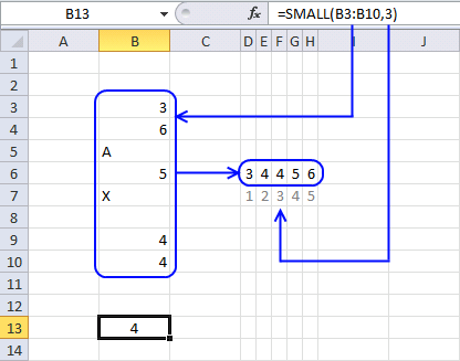
The image above shows a formula in cell B13 that extracts the third smallest value from cell range B3:B10. Note that the cell range contains both text values and blank cells.
becomes
SMALL({3; 6; "A"; 5; "X"; 0; 4; 4}, 3)
Text strings and blanks are overlooked. The array becomes
SMALL({3; 6; ; 5; ; ; 4; 4}, 3)
and returns 4. 4 is the third smallest numerical value in the array.
4. How to use constants (hardcoded) values

In case you want to work with an array instead of a cell range in the SMALL function use curly brackets like this:
This means that the values are hardcoded into the formula, however, you still enter it as a regular formula.
There is one downside with this approach and that is that you must edit the formula to be able to change a value in the array.
To convert a cell range to an array select the cell reference in the formula and press function key F9.

This will convert the cell range to an array of values.
5. How to use a condition
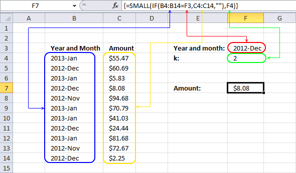
This array formula in cell F7 calculates the second smallest number from cell range C4:C14 based on a condition specified in cell F3.
The IF function returns one value if the logical test returns TRUE and another value if the logical test is FALSE.
IF(logical_test, [value_if_true], [value_if_false])
In this case, the IF function compares the values in cell range B4:B14 to the value in cell F3 and returns and an array that contains boolean values TRUE or FALSE.
SMALL(IF(B4:B14=F3, C4:C14, ""), F4)
becomes
SMALL(IF({"2013-Jan"; "2012-Dec"; "2013-Jan"; "2012-Dec"; "2012-Nov"; "2013-Jan"; "2013-Jan"; "2012-Dec"; "2013-Jan"; "2012-Nov"; "2012-Dec"}="2012-Dec", C4:C14, ""), F4)
becomes
SMALL(IF({FALSE; TRUE; FALSE; TRUE; FALSE; FALSE; FALSE; TRUE; FALSE; FALSE; TRUE}, C4:C14, ""), F4)
The IF function then returns the corresponding value from the second argument if TRUE and the third argument if FALSE.
SMALL(IF({FALSE; TRUE; FALSE; TRUE; FALSE; FALSE; FALSE; TRUE; FALSE; FALSE; TRUE}, C4:C14, ""), F4)
becomes
SMALL(IF({FALSE; TRUE; FALSE; TRUE; FALSE; FALSE; FALSE; TRUE; FALSE; FALSE; TRUE},{55.47; 60.69; 5.83; 8.08; 94.68; 70.79; 41.03; 24.44; 81.68; 72.67; 2.25},""), F4)
becomes
SMALL({"";60.69;"";8.08;"";"";"";24.44;"";"";2.25}, 2)
and returns 8.08 in cell F7.
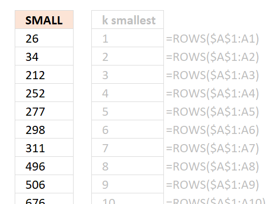
6. How to quickly return sorted numbers

Formula in cell E3:
The second argument k can be changed from a number to a function that returns numbers, this can be handy when you want to return multiple numbers sorted from small to large.
SMALL(array, k )
The ROWS function returns the number of rows a cell range contains. If you combine absolute and relative references into one cell reference you can build a dynamic cell reference that changes when you copy the cell and paste to cells below.
$A$1:A1
The first part of the cell reference is absolute meaning it won't change when the cell is copied and pasted to cells below. You can see that it is absolute bu the $ dollar signs in front of the column letter and the row number.
The colon is used to describe a cell range that contains multiple cells however it can also describe a reference to a single cell. The second part is relative meaning it will change when you copy the cell.
For example, the table below demonstrates how the cell references in the formula change when copied.
Cell E3: =SMALL($B$3:$B$11, ROWS($A$1:A1))
Cell E4: =SMALL($B$3:$B$11, ROWS($A$1:A2))
Cell E5: =SMALL($B$3:$B$11, ROWS($A$1:A3))
The cell range expands by one row for each new cell below you paste it to. The ROWS function calculates the number of rows in that cell range and returns that number.
Cell E3: =SMALL($B$3:$B$11, 1)
Cell E4: =SMALL($B$3:$B$11, 2)
Cell E5: =SMALL($B$3:$B$11, 3)

You can press and hold on the black dot in the bottom right corner of the selected cell then drag down as far as needed to quickly copy the cell to cells below, see animated image above.

You can also double press with left mouse button on with left mouse button on the black dot located in the bottom right corner of the selected cell to quickly copy the cell to cells below.
Excel uses existing values in the adjacent column to determine when to stop copying.
7. Multiple cell ranges
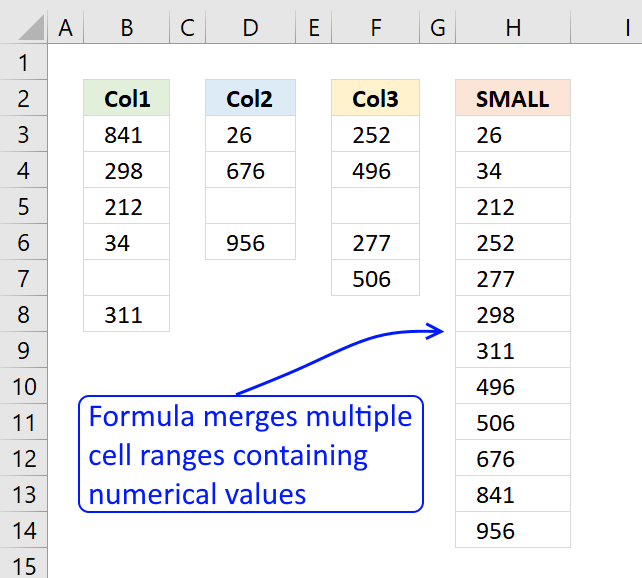
Today I learned how to sort numbers from multiple cell ranges thanks to Sam Miller. It is surprisingly simple and easy.
Formula in cell H3:
The SMALL function ignores text and blank cells, however, not error values.
Explaining formula in cell H3
Step 1 - Enable multiple cell ranges
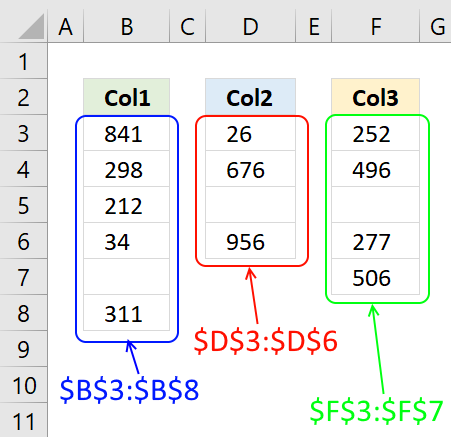
The first argument in the SMALL function is the array parameter: SMALL(array, k).
Use parentheses to enable multiple cell ranges in the first argument.
($B$3:$B$8, $D$3:$D$6, $F$3:$F$7)
The , (comma) separates the cell references.
Step 2 - Extract k-th smallest number
The second argument allows you to specify which number to extract based on their sort order.
ROWS($A$1:A1)
The ROWS function allows you to insert new rows and columns in your worksheet without breaking the formula.
The cell reference contains two parts, one is an absolute cell reference and the other is a relative cell reference.
The $ sign allows you to specify an absolute cell reference, this cell reference does not change when you copy the formula to cells below.
Get Excel *.xlsx file
SMALL function with multiple cell ranges.xlsx
8. How to ignore error values
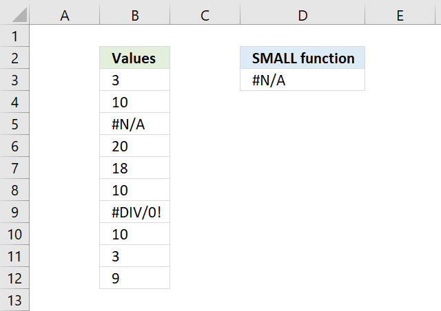
The image above shows you a formula in cell D3 that tries to get the smallest number from cell range B3:B12 but it returns an error. This happens if the cell range contains at least one error value.
Formula in cell D3:
The SMALL function ignores text and boolean values but not error values, however, the AGGREGATE function lets you choose between a variety of functions (including SMALL function).
You also have the option to ignore error values, the second argument lets you specify this.
The AGGREGATE function contains these functions AVERAGE, COUNT, COUNTA, MAX, MIN, PRODUCT, STDEV.S, STDEV.P, SUM, VAR.S, VAR.P, MEDIAN, MODE.SNGL, LARGE, SMALL, PERCENTILE.INC, QUARTILE.INC, PERCENTILE.EXC and QUARTILE.EXC.
You can see a list of available functions while entering the arguments in the function, see image below.
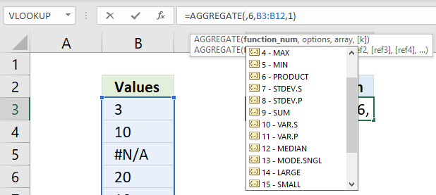
The second argument has the following settings, I chose 6 - Ignore error values.
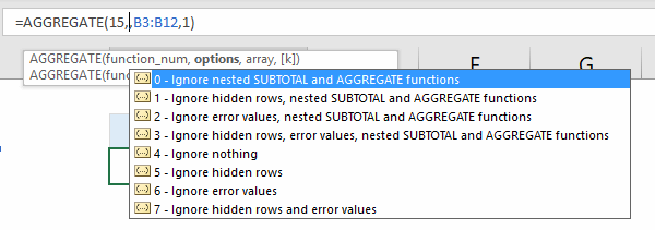
The AGGREGATE function was introduced in Excel 2010, if you have an earlier Excel version then I recommend using the following array formula:
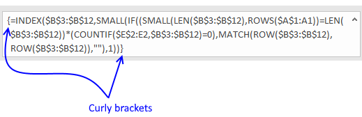
To enter an array formula, type the formula in a cell then press and hold CTRL + SHIFT simultaneously, now press Enter once. Release all keys.
The formula bar now shows the formula with a beginning and ending curly bracket telling you that you entered the formula successfully. Don't enter the curly brackets yourself.
9. INDEX MATCH

The array formula in cell C11 gets 3 values in one fetch, the INDEX function allows you to do that if you enter 0 (zero) in the row or column argument. The SMALL function then calculates the k-th smallest value of these three values.
9.1 How to enter an array formula
To enter an array formula, type the formula in a cell then press and hold CTRL + SHIFT simultaneously, now press Enter once. Release all keys.
The formula bar now shows the formula with a beginning and ending curly bracket telling you that you entered the formula successfully. Don't enter the curly brackets yourself.
9.2 Explaining formula in cell C11
Step 1 - Find the relative position of condition in B3:B7
The MATCH function returns the location of a specified value in an array och cell range.
MATCH(lookup_value, lookup_array, [match_type])
MATCH($C$10, $B$3:$B$7, 0) returns 3. Value D is found in position 3 in the array.
Step 2 - Get values based on relative position
The INDEX function returns a value from a cell range, you specify which value based on a row and column number. It can also return multiple values if you use 0 (zero) in the row or column argmunets or both.
INDEX($C$3:$E$7, MATCH($C$10, $B$3:$B$7, 0), 0) becomes INDEX($C$3:$E$7, 3, 0)
The INDEX function then returns all values on relative row 3 in this cell range $C$3:$E$7: {590, 830, 280}
Step 3 - Extract k-th smallest number
The SMALL function returns the k-th smallest value from a group of numbers.
SMALL(array, k)
SMALL(INDEX($C$3:$E$7, MATCH($C$10, $B$3:$B$7, 0), 0), ROWS($A$1:A1))
ROWS($A$1:A1) returns the number of rows in cell reference $A$1:A1, it grows when you copy the cell and paste it to cells below. This makes the formula extract a new number in each cell below.
SMALL(INDEX($C$3:$E$7, MATCH($C$10, $B$3:$B$7, 0), 0), ROWS($A$1:A1)) returns 280 in cell C11.
You can also use the SMALL function to match multiple values, make sure you read this post: 5 easy ways to VLOOKUP and return multiple values
10. INDEX MATCH - Excel 365

The formula in cell C11 extracts numbers from a row that has a value that meets the condition. It then sorts the numbers from small to large.
Formula in cell C11:
10.1 Explaining formula in cell C11
Step 1 - Identify values that meet the condition
The equal sign lets you compare value to value, in this case, value to an array of values. The result is a boolean value TRUE or FALSE and the resulting array is equal in size to the array we compared.
B3:B7=C10 returns {FALSE; FALSE; TRUE; FALSE; FALSE}.
Step 2 - Filter numbers
The FILTER function lets you extract values/rows based on a condition or criteria.
FILTER(array, include, [if_empty])
FILTER(C3:E7, B3:B7=C10) returns {590, 830, 280}.
Note that the numbers are comma-delimited meaning they are arranged horizontally.
Step 3 - Transpose values
The TRANSPOSE function allows you to convert a vertical range to a horizontal range, or vice versa.
TRANSPOSE(array)
TRANSPOSE(FILTER(C3:E7,B3:B7=C10)) returns {590; 830; 280}.
Step 4 - Sort values
The SORT function lets you sort values from a cell range or array.
SORT(array, [sort_index], [sort_order], [by_col])
SORT(TRANSPOSE(FILTER(C3:E7,B3:B7=C10))) returns {280; 590; 830}.
Get Excel *.xlsx file
SMALL function - INDEX - MATCH.xlsx
11. How to ignore zeros
This section shows how to create a formula that sorts numbers from small to large excluding zeros. I will also demonstrate a formula ignoring negative values and then sort from small to large.
Table of contents - section 11
- SMALL function - ignore zeros (array formula)
- SMALL function - ignore zeros (regular formula)
- SMALL function - ignore zeros (Excel 365)
- SMALL function - ignore negative numbers
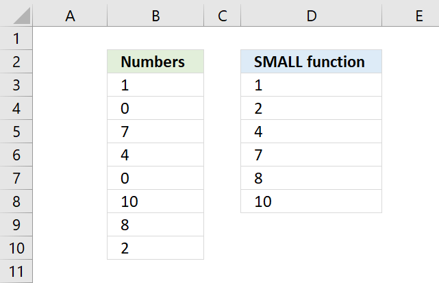
11.1. How to ignore zeros - array formula
The formula in cell D3 is an array formula, it will extract the k-th smallest value ignoring zeros.
11.2 How to enter an array formula

To enter an array formula, type the formula in a cell then press and hold CTRL + SHIFT simultaneously, now press Enter once. Release all keys.
The formula bar now shows the formula with a beginning and ending curly bracket telling you that you entered the formula successfully. Don't enter the curly brackets yourself.
11.3 Explaining formula
Step 1 - Logical test
The equal sign lets you compare value to value, the result is a boolean value TRUE or FALSE. This is called a logical expression or a logical test. We will use this in the next step to filter out numbers that don't meet the condition.
$B$3:$B$10=0 returns {FALSE; TRUE; FALSE; ... ; FALSE}.
Step 2 - Replace TRUE with the corresponding value
The IF function then returns the corresponding values from column D if TRUE and a blank "" if FALSE.
IF(logical_test, [value_if_true], [value_if_false])
IF($B$3:$B$10=0, "", $B$3:$B$10) returns .{1; ""; 7; 4; ""; 10; 8; 2}
If the value is 0 (zero) the IF function returns a blank "" in that position in the array and if not 0 (zero) the IF function returns the number.
Step 3 - Replace TRUE with the corresponding value
The SMALL function returns the k-tk smallest value the array determined by ROWS($A$1:A1).
SMALL(array, k)
The ROWS function makes this formula dynamic, in cell D3 the ROWS function returns 1. Copy the cell to next cell below and it changes to ROWS($A$1:A2) and returns 2 making it return the second smallest value in the array in cell D4.
SMALL({1; ""; 7; 4; ""; 10; 8; 2}, ROWS($A$1:A1)) returns 1 in cell D3.
11.4. How to ignore zeros - regular formula
If you want to avoid an array formula then try this formula in cell D3:
11.4.1 Explaining formula
Step 1 - Find numbers not equal to 0 (zero)
The less than and the larger than signs combined lets you test if a value is not equal to a condition, in this case, 0 (zero).
$B$3:$B$10<>0 returns {TRUE; FALSE; TRUE; ... ; TRUE}.
Step 2 - Divide numbers by a boolean array
The forward slash character lets you divide a number by another number in an Excel formula. This works fine with boolean values TRUE and FALSE as well.
TRUE = 1
FALSE = 0 (zero)
$B$3:$B$10/($B$3:$B$10<>0) returns {1; #DIV/0!; 7; 4; #DIV/0!; 10; 8; 2}.
Notice how some values are actually error values in the array above. This is because when you divide with FALSE which is equivalent with 0 (zero) and that returns a #DIV/0! error. It is not possible to divide a number by zero.
Step 3 - Extract k-th smallest number
The AGGREGATE function performs different specific functions to a list or database.
Array form
AGGREGATE(function_num, options, array, [k])
function_num - 15 (SMALL function)
options - 6 (ignore error values)
AGGREGATE(15,6,$B$3:$B$10/($B$3:$B$10<>0),ROWS($A$1:A1)) becomes AGGREGATE(15,6,{1; #DIV/0!; 7; 4; #DIV/0!; 10; 8; 2}, 1)
and returns 1.
11.5. Ignore zeros - Excel 365
The formula in cell D3 is an Excel 365 formula containing new functions, they are the SORT and FILTER functions.
These functions let you filter all numbers except zeros and sort them from small to large.
Dynamic array formula in cell D3:
A dynamic array formula spills values to adjacent cells automatically if the result is an array of values, it is entered as a regular formula.
11.5.1 Explaining formula
Step 1 - Identify values not equal to zero
The equal sign lets you compare value to value, the result is a boolean value TRUE or FALSE. This is called a logical expression or a logical test. We will use this in the next step to filter out numbers that don't meet the condition.
B3:B10<>0 returns {TRUE; FALSE; TRUE; ... ; TRUE}.
Step 2 - Filter out zeros
The FILTER function lets you extract values/rows based on a condition or criteria.
FILTER(array, include, [if_empty])
FILTER(B3:B10, B3:B10<>0) returns {1; 7; 4; 10; 8; 2}.
Step 3 - Sort from small to large
The SORT function lets you sort values from a cell range or array. It returns an array with a size that matches the number of values in the array argument.
SORT(FILTER(B3:B10, B3:B10<>0)) returns {1; 2; 4; 7; 8; 10}.
11.6. Ignore negative numbers

The formula in cell D3 extracts all numbers except numbers smaller than 0 (zero), in other words, ignoring negative numbers.
Array formula in cell D3:
Get Excel file
12. Multiple conditions - example 2
This section demonstrates how to sort numbers from small to large using a condition or criteria, I will show how both AND and OR logic works, and using values and rows/records.
Table of Contents
- SMALL function - multiple conditions AND logic
- SMALL function - multiple conditions OR logic
- SMALL function - match records AND logic
- SMALL function - match records OR logic
- SMALL function - match multiple values OR logic
- Get Excel *.xlsx file
12.1. Multiple conditions AND logic
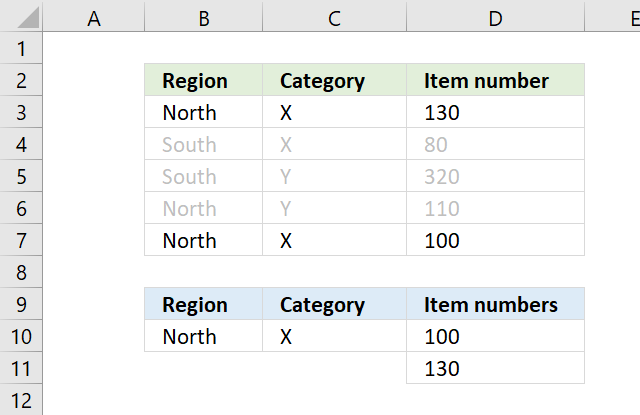
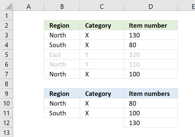
The array formula in D10 extracts numbers sorted from small to large from column D if Region is equal to North AND Category is X on the same row.
12.1.1 How to enter an array formula
Excel 365 users can ignore these instructions, enter the formula as a regular formula. To enter an array formula, type the formula in a cell then press and hold CTRL + SHIFT simultaneously, now press Enter once. Release all keys.
The formula bar now shows the formula with a beginning and ending curly bracket telling you that you entered the formula successfully. Don't enter the curly brackets yourself.
12.1.2 Explaining formula
Step 1 - First condition
The equal sign compares value to value in Excel, this works fine with a value to multiple values as well. The result is either TRUE or FALSE.
$B$10=$B$3:$B$7
and returns
TRUE; FALSE; FALSE; TRUE; TRUE}
Step 2 - Second condition
$C$10=$C$3:$C$7
and returns
{TRUE; TRUE; FALSE; FALSE; TRUE}
Step 3 - Multiply arrays AND logic
There are two logical expressions in the formula returning boolean values TRUE or FALSE.
($B$10=$B$3:$B$7)*($C$10=$C$3:$C$7)
The asterisk between the logical expressions multiply the boolean arrays, this will help us extract numbers where both conditions match on the same row.
{TRUE; FALSE; FALSE; TRUE; TRUE}) * ({TRUE; TRUE; FALSE; FALSE; TRUE}
and returns {1; 0; 0; 0; 1}.
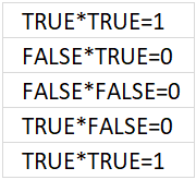
The result is either 0 (zero) or 1, the numerical equivalent of TRUE is 1 and FALSE is 0 (zer0).
Step 4 - Replace TRUE with corresponding number on the same row
The IF function then returns the corresponding values from column D if TRUE and a blank "" if FALSE.
IF(($B$10=$B$3:$B$7)*($C$10=$C$3:$C$7), $D$3:$D$7, "")
becomes
IF({1; 0; 0; 0; 1}, {130; 80; 320; 110; 100}, "")
and returns
{130; ""; ""; ""; 100}.
Step 5 - Extract k-th smallest number
The SMALL function returns the k-tk smallest value the array determined by ROWS($A$1:A1).
SMALL(IF(($B$10=$B$3:$B$7)*($C$10=$C$3:$C$7), $D$3:$D$7, ""), ROWS($A$1:A1))
becomes
SMALL({130; ""; ""; ""; 100}, ROWS($A$1:A1))
The cell reference in ROWS($A$1:A1) expands when you copy the cell and paste it to cells below.
The smallest value is shown in D10, ROWS($A$1:A1) returns 1. The second smallest value is shown in D11, ROWS($A$1:A2) returns 2.
The ROWS function has a great advantage, it won't break the formula if you insert or delete rows above the array formula.
SMALL({130; ""; ""; ""; 100}, ROWS($A$1:A1))
becomes
SMALL({130; ""; ""; ""; 100}, 1)
and returns 100 in cell D10.
12.2. Multiple conditions OR logic
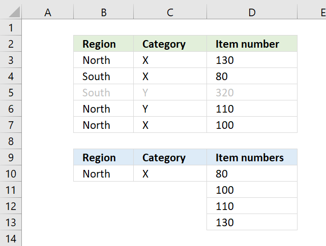
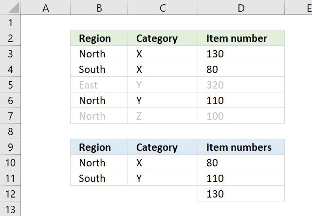
The array formula in D10 extracts numbers sorted from small to large from column D if Region is equal to North OR Category is X.
Explaining formula
Step 1 - First condition
The equal sign compares value to value in Excel, this works fine with a value to multiple values as well. The result is either TRUE or FALSE.
$B$10=$B$3:$B$7
returns {TRUE; FALSE; FALSE; TRUE; TRUE}.
Step 2 - Second condition
$C$10=$C$3:$C$7
returns {TRUE; TRUE; FALSE; FALSE; TRUE}.
Step 3 - Add arrays
The plus sign lets you add a number with another number, you can also add arrays as long as they contain the same number of values.

If you add the logical expressions you get what the image above shows. All numbers except 0 (zero) equal TRUE and 0 (zero) is FALSE.
($B$10=$B$3:$B$7)+($C$10=$C$3:$C$7) returns {2; 1; 0; 1; 2}.
Step 4 - Replace TRUE with corresponding number on the same row
The IF function then returns the corresponding values from column D if TRUE and a blank "" if FALSE.
IF(logical_test, [value_if_true], [value_if_false])
IF(($B$10=$B$3:$B$7)+($C$10=$C$3:$C$7), $D$3:$D$7, "")
returns {130; 80; ""; 110; 100}.
Step 5 - Extract k-th smallest number
The SMALL function returns the k-tk smallest value the array determined by ROWS($A$1:A1).
SMALL(array, k)
SMALL(IF(($B$10=$B$3:$B$7)+($C$10=$C$3:$C$7), $D$3:$D$7, ""), ROWS($A$1:A1))
becomes SMALL({130; 80; ""; 110; 100}, 1) and returns 80.
12.3. Match records AND logic
The formula above in D10 extracts numbers sorted from small to large if both Region and Category match on the same row in both tables.
This formula is similar to the first formula, however, the COUNTIFS function allows you to easily use multiple criteria without building huge formulas.
12.3.1 Explaining formula
Step 1 - Find matching rows
The COUNTIFS function calculates the number of cells across multiple ranges that equals all given conditions.
COUNTIFS(criteria_range1, criteria1, [criteria_range2, criteria2]…)
COUNTIFS($B$10:$B$11,$B$3:$B$7, $C$10:$C$11,$C$3:$C$7)
returns {1; 1; 0; 0; 1}.
Step 2 - Replace any number except zero with corresponding number on the same row
The IF function then returns the corresponding values from column D if TRUE and a blank "" if FALSE.
IF(logical_test, [value_if_true], [value_if_false])
TRUE - any number except zero
FALSE - 0 (zero)
IF(COUNTIFS($B$10:$B$11,$B$3:$B$7, $C$10:$C$11,$C$3:$C$7), $D$3:$D$7, "")
returns {130; 80; ""; ""; 100}.
Step 3 - Extract k-th smallest number
The SMALL function returns the k-tk smallest value the array determined by ROWS($A$1:A1).
SMALL(array, k)
SMALL(IF(COUNTIFS($B$10:$B$11,$B$3:$B$7, $C$10:$C$11,$C$3:$C$7), $D$3:$D$7, ""), ROWS($A$1:A1))
returns 80 in cell D10.
12.4. Match records OR logic
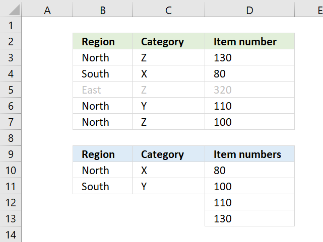
The formula above in D10 extracts numbers sorted from small to large if both Region and Category match any of the criteria.
Example, Z on row 7 is not a match to any of the Category values in the lower table, both values must match.
12.4.1 Explaining formula
Step 1 - Count cells based on criteria in B10 and B11
The COUNTIF function calculates the number of cells that is equal to a condition.
COUNTIF(range, criteria)
COUNTIF($B$10:$B$11, $B$3:$B$7)
returns {1; 1; 0; 1; 1}.
Step 2 - Count cells based on criteria in C10 and C11
COUNTIF($C$10:$C$11, $C$3:$C$7)
{1; 1; 1; 1; 0}.
Step 3 - Multiply arrays
Multiply the arrays to create AND logic, here is how it works:
1 * 1 = 1 (TRUE)
1*0 = 0 (FALSE)
0*0 = 0 (FALSE)
COUNTIF($B$10:$B$11, $B$3:$B$7)*COUNTIF($C$10:$C$11, $C$3:$C$7)
becomes
{1; 1; 0; 1; 1} * {1; 1; 1; 1; 0}
equals {1; 1; 0; 1; 0}.
Step 4 - REPLACE 1 (TRUE) with corresponding number on the same row
The IF function then returns the corresponding values from column D if TRUE and a blank "" if FALSE.
IF(logical_test, [value_if_true], [value_if_false])
IF(COUNTIF($B$10:$B$11, $B$3:$B$7)*COUNTIF($C$10:$C$11, $C$3:$C$7), $D$3:$D$7, "")
returns {130; 80; ""; 110; ""}.
Step 5 - Extract k-th smallest number
The SMALL function returns the k-tk smallest value the array determined by ROWS($A$1:A1).
SMALL(array, k)
SMALL(IF(COUNTIF($B$10:$B$11, $B$3:$B$7)*COUNTIF($C$10:$C$11, $C$3:$C$7), $D$3:$D$7, ""), ROWS($A$1:A1))
becomes
SMALL({130; 80; ""; 110; ""}, 1) and returns 80.
12.5. Match multiple values OR logic
The formula above in D10 extracts numbers sorted from small to large if any of the Region or Category values match.
12.5.1 Explaining formula
Step 1 - Count cells based on criteria in B10 and B11
The COUNTIF function calculates the number of cells that is equal to a condition.
COUNTIF(range, criteria)
COUNTIF($B$10:$B$11, $B$3:$B$7)
returns {1; 1; 0; 1; 1}.
Step 2 - Count cells based on criteria in C10 and C11
COUNTIF($C$10:$C$11, $C$3:$C$7)
returns {0; 1; 0; 1; 0}.
Step 3 - Add arrays
The plus sign lets you add numbers in an Excel formula, this works fine with arrays as well.
COUNTIF($B$10:$B$11, $B$3:$B$7)+ COUNTIF($C$10:$C$11, $C$3:$C$7)
returns {1; 2; 0; 2; 1}.
Step 4 - Replace 1 (True) with corresponding number on the same row
The IF function then returns the corresponding values from column D if TRUE and a blank "" if FALSE.
IF(logical_test, [value_if_true], [value_if_false])
IF(COUNTIF($B$10:$B$11, $B$3:$B$7)+ COUNTIF($C$10:$C$11, $C$3:$C$7), $D$3:$D$7, "")
returns {130; 80; ""; 110; 100}.
Step 5 - Extract k-th smallest number
The SMALL function returns the k-tk smallest value the array determined by ROWS($A$1:A1).
SMALL(array, k)
SMALL(IF(COUNTIF($B$10:$B$11, $B$3:$B$7)+ COUNTIF($C$10:$C$11, $C$3:$C$7), $D$3:$D$7, ""), ROWS($A$1:A1))
returns 80 in cell D10.
12.6 Get Excel *.xlsx file
SMALL function - multiple critera.xlsx
13. For text
This section demonstrates a formula that sorts text values based on character length, the Excel 365 dynamic array formula is considerably smaller and is a great example of how amazing the new Excel 365 functions are.
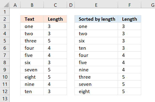
The image above shows the result in cell E3 and cells below, the formula is returning values from cell range B3:B12 from small to large (ascending order). Cell range C3:C12 shows the string length of the corresponding cell on the same row.
Table of Contents
- SMALL function for text
- SMALL function for text - Excel 365
- Get Excel *.xlsx file
12.1. For text - example 1
The array formula in column E, shown in above picture sorts text values from column B. The Length columns prove that they are sorted by text length from small to large. Don't use this formula if you are an Excel 365 subscriber, read section 2.
12.1.1 How to enter an array formula
To enter an array formula, type the formula in a cell then press and hold CTRL + SHIFT simultaneously, now press Enter once. Release all keys.
The formula bar now shows the formula with a beginning and ending curly bracket telling you that you entered the formula successfully. Don't enter the curly brackets yourself.
12.1.2 Explaining formula
Step 1 - Calculate string length
The LEN function returns a number representing the number of characters in a given cell.
LEN(text)
LEN($B$3:$B$12)
becomes
LEN({"one"; "two"; "three"; "four"; "five"; "six"; "seven"; "eight"; "nine"; "ten"})
and returns
{3; 3; 5; 4; 4; 3; 5; 5; 4; 3}.
Step 2 - Extract the k-th smallest number
The SMALL function returns the k-th smallest value from a group of numbers.
SMALL(array, k)
SMALL(LEN($B$3:$B$12), ROWS($A$1:A1))
becomes
SMALL({3; 3; 5; 4; 4; 3; 5; 5; 4; 3}, ROWS($A$1:A1))
The ROWS function allows you to calculate the number of rows in a cell range.
ROWS(array)
The cell reference $A$1:A1 has two parts, an absolute and a relative part. When you copy the cell and paste it to the cells below the relative part changes accordingly. This will calculate a new number in each cell, the first cell evaluates to 1, the next cell below evaluates to two, and so on.
SMALL({3; 3; 5; 4; 4; 3; 5; 5; 4; 3}, ROWS($A$1:A1))
becomes
SMALL({3; 3; 5; 4; 4; 3; 5; 5; 4; 3}, 1)
and returns 3.
Step 3 - Compare the result to the array
The equal sign is a logical operator, it allows you to compare value to value or in this case value to an array. The result is a boolean value, TRUE or FALSE.
SMALL(LEN($B$3:$B$12), ROWS($A$1:A1))=LEN($B$3:$B$12)
becomes
3=LEN($B$3:$B$12)
becomes
3={3; 3; 5; 4; 4; 3; 5; 5; 4; 3}
and returns
{TRUE; TRUE; FALSE; FALSE; FALSE; TRUE; FALSE; FALSE; FALSE; TRUE}.
Step 4 - Count previous results above and compare result with zero
The COUNTIF function calculates the number of cells that is equal to a condition.
COUNTIF(range, criteria)
(COUNTIF($E$2:E2, $B$3:$B$12)=0
becomes
{0;0;0;0;0;0;0;0;0;0}=0
and returns
{TRUE; TRUE; TRUE; TRUE; TRUE; TRUE; TRUE; TRUE; TRUE; TRUE}.
This means that there have not been displayed any values above yet.
Step 5 - Multiply arrays
We will now multiply the array containing character length with the array containing where the k-th smallest number is.
(SMALL(LEN($B$3:$B$12), ROWS($A$1:A1))=LEN($B$3:$B$12))*(COUNTIF($E$2:E2, $B$3:$B$12)=0)
becomes
{TRUE; TRUE; FALSE; FALSE; FALSE; TRUE; FALSE; FALSE; FALSE; TRUE}*(COUNTIF($E$2:E2, $B$3:$B$12)=0)
becomes
{TRUE; TRUE; FALSE; FALSE; FALSE; TRUE; FALSE; FALSE; FALSE; TRUE}*{TRUE; TRUE; TRUE; TRUE; TRUE; TRUE; TRUE; TRUE; TRUE; TRUE}
and returns
{1; 1; 0; 0; 0; 1; 0; 0; 0; 1}.
When you perform a calculation to boolean values the result is always the numerical equivalent.
TRUE = 1 and FALSE = 0 (zero)
Step 6 - Replace TRUE with corresponding row number
The IF function returns one value if the logical test is TRUE and another value if the logical test is FALSE.
IF(logical_test, [value_if_true], [value_if_false])
IF((SMALL(LEN($B$3:$B$12), ROWS($A$1:A1))=LEN($B$3:$B$12))*(COUNTIF($E$2:E2, $B$3:$B$12)=0), MATCH(ROW($B$3:$B$12), ROW($B$3:$B$12)), "")
becomes
IF({1; 1; 0; 0; 0; 1; 0; 0; 0; 1}, MATCH(ROW($B$3:$B$12), ROW($B$3:$B$12)), "")
The ROW and MATCH function combined creates a sequence of numbers from 1 to n where n is the number of rows in $B$3:$B$12
MATCH(ROW($B$3:$B$12), ROW($B$3:$B$12))
becomes
MATCH({3;4;5;6;7;8;9;10;11;12}, {3;4;5;6;7;8;9;10;11;12})
and returns
{1; 2; 3; 4; 5; 6; 7; 8; 9; 10}.
IF({1; 1; 0; 0; 0; 1; 0; 0; 0; 1}, MATCH(ROW($B$3:$B$12), ROW($B$3:$B$12)), "")
becomes
IF({1; 1; 0; 0; 0; 1; 0; 0; 0; 1}, {1; 2; 3; 4; 5; 6; 7; 8; 9; 10}, "")
and returns
{1; 2; ""; ""; ""; 6; ""; ""; ""; 10}.
Step 7 - Extract the smallest row number
SMALL(IF((SMALL(LEN($B$3:$B$12), ROWS($A$1:A1))=LEN($B$3:$B$12))*(COUNTIF($E$2:E2, $B$3:$B$12)=0), MATCH(ROW($B$3:$B$12), ROW($B$3:$B$12)), ""), 1)
becomes
SMALL({1; 2; ""; ""; ""; 6; ""; ""; ""; 10}, 1)
and returns 1.
Step 8 - Get value
The INDEX function returns a value from a cell range, you specify which value based on a row and column number.
INDEX($B$3:$B$12, SMALL(IF((SMALL(LEN($B$3:$B$12), ROWS($A$1:A1))=LEN($B$3:$B$12))*(COUNTIF($E$2:E2, $B$3:$B$12)=0), MATCH(ROW($B$3:$B$12), ROW($B$3:$B$12)), ""), 1))
becomes
INDEX($B$3:$B$12, 1)
and returns "one" in cell F3.
If you are looking for a formula that sorts text alphabetically, check this out: Sort a column alphabetically
12.2. For text - Excel 365
The formula in cell E3 sorts the text values in cell range B3:B12 based on character length from small to large.
Dynamic array formula in cell E3:
12.2.1 How to enter a dynamic array formula
The formula in cell E3 works only in Excel 365, it is entered as a regular formula however, it spills to cells below as far as needed.
12.2.2 Explaining formula
Step 1 - Calculate string length
The LEN function returns a number representing the number of characters in a given cell.
LEN(text)
LEN(B3:B12)
becomes
LEN({"one"; "two"; "three"; "four"; "five"; "six"; "seven"; "eight"; "nine"; "ten"})
and returns
{3; 3; 5; 4; 4; 3; 5; 5; 4; 3}.
Step 2 - Sort by string length
The SORTBY function allows you to sort values from a cell range or array based on a corresponding cell range or array. It sorts values by column but keeps rows.
SORTBY(array, by_array1, [sort_order1], [by_array2, sort_order2],…)
SORTBY(B3:B12, LEN(B3:B12), 1)
becomes
SORTBY(B3:B12, {3; 3; 5; 4; 4; 3; 5; 5; 4; 3}, 1)
and returns
{"one"; "two"; "six"; "ten"; "four"; "five"; "nine"; "three"; "seven"; "eight"}.
12.3 Get Excel file
14. Ignore duplicates
This section demonstrates ways to sort numbers from smallest to largest ignoring duplicate numbers.
Table of Contents
- SMALL function with duplicates (Excel 2016)
- SMALL function with duplicates (previous Excel versions)
- SMALL function with duplicates (Excel 365)
- SMALL function with duplicates based on a condition
- Get Excel *.xlsx file
14.1. Duplicates (Excel 2016)
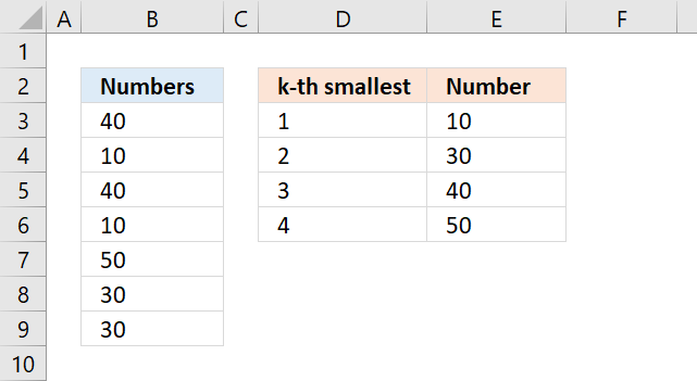
The formulas in column E, shown in the picture above, extract the k-th smallest value from B3:B9 ignoring the duplicate numbers.
The following formula in cell E3 extracts the smallest number:
However, we need to use another formula in the cells below to ignore duplicate values. The formula in cell E4 extracts the second smallest number from B3:B9.
When you copy this formula and paste it to cells below it will extract the third, fourth, and so on, smallest value ignoring duplicate values.
The MINIFS function returns the smallest value depending on the condition, in this case, it looks for values larger than the previous value in the cell above, meaning it will ignore duplicate numbers.
I can't use this formula in cell E3 because there is no formula above it.
The MINIFS function was introduced in Excel 2016, if you have an earlier version of Excel see section 2 below.
14.1.1 Explaining formula
Step 1 - MINIFS function
The MINIFS function calculates the smallest value based on a given set of criteria.
MINIFS(min_range, criteria_range1, criteria1, [criteria_range2, criteria2], ...)
| min_range | Required. A cell reference pointing to the numbers. |
| criteria_range1 | Required. Cells to evaluate based on the criteria. |
| criteria1 | Required. Criteria in the form of a number, expression, or text. |
| [criteria_range2] | Optional. Up to 126 additional arguments. |
| [criteria2] | Optional. Up to 126 additional arguments. |
Step 2 - Populate arguments
min_range - $B$3:$B$9
criteria_range1 - $B$3:$B$9
criteria1 - ">"&E3
MINIFS($B$3:$B$9, $B$3:$B$9, ">"&E3)
Step 3 - Evaluate formula
MINIFS($B$3:$B$9, $B$3:$B$9, ">"&E3)
becomes
MINIFS({40; 10; 40; 10; 50; 30; 30},{40; 10; 40; 10; 50; 30; 30},">"&10)
and returns 30 in cell E4.
Note, it won't return duplicate numbers when you copy cell E4 and paste it to the cells below.
14.2. Duplicates - previous Excel versions
Formula in cell E3:
Array formula in cell E4:
The formula above is an array formula.
14.2.1 How to enter an array formula
To enter an array formula, type the formula in a cell then press and hold CTRL + SHIFT simultaneously, now press Enter once. Release all keys.
The formula bar now shows the formula enclosed with curly brackets telling you that you entered the formula successfully. Don't enter the curly brackets yourself.
Explaining array formula
Step 1 - Check which numbers are larger than cell E3
The less than sign is a logical operator, it allows you to compare numbers and text strings. The result is either TRUE or FALSE, they are boolean values and will be used in step 2 in an IF functions logical test argument.
E3<$B$3:$B$9
returns {TRUE; FALSE; TRUE; FALSE; TRUE; TRUE; TRUE}.
Step 2 - Filter numbers based on logical test
The IF function returns one value if the logical test is TRUE and another value if the logical test is FALSE.
IF(logical_test, [value_if_true], [value_if_false])
IF(E3<$B$3:$B$9, $B$3:$B$9, "")
returns {40; ""; 40; ""; 50; 30; 30}
Numbers smaller than or equal to the condition are filtered out from the array.
Step 3 - Extract the smallest number from the array
The MIN function returns the smallest number from a cell range or array ignoring text and blank values.
MIN(IF(E3<$B$3:$B$9, $B$3:$B$9, ""))
becomes MIN({40; ""; 40; ""; 50; 30; 30}) and returns 30 in cell E3.
14.3. Duplicates - Excel 365

Formula in cell E3:
14.3.1 Explaining formula
Step 1 - Extract unique distinct values
The UNIQUE function returns unique distinct numbers.
UNIQUE(B3:B9)
returns {40; 10; 50; 30}.
Step 2 - Sort values from small to large
The SMALL function returns the k-th smallest number.
SMALL(array, k)
SMALL(UNIQUE(B3:B9),ROWS($A$1:A1))
becomes
SMALL({40; 10; 50; 30},ROWS($A$1:A1))
The ROWS function returns the number of rows based on the specified cell reference.
ROWS(ref)
The reference $A$1:A1 contains an absolute part and a relative part, the absolute part stays the same, however, the relative part changes when you copy the cell and paste it to cells below.
SMALL({40; 10; 50; 30},1) and returns 10 in cell E3.
14.4. Ignore duplicates based on a condition

The image above demonstrates two formulas that let you extract the smallest number based on a condition ignoring duplicate numbers.
The formula in cell F5 extracts the smallest number based on a condition specified in cell F2, however, this formula works only in the first cell. Cell F6 and cells below require a different formula.
The array formulas below work in all Excel versions, here is how to enter an array formula.
Array formula in cell F5:
Array formula in cell F6:
Copy cell F6 and paste it to cells below as far as needed.
14.4.1 Explaining formula in cell F5
Step 1 - Logical test
The equal sign is a logical operator and the result is a boolean value, TRUE or FALSE.
$F$2=$B$3:$B$9
returns {TRUE; TRUE; ... ; TRUE}.
Step 2 - Evaluate IF function
The IF function returns one value if the logical test is TRUE and another value if the logical test is FALSE.
IF(logical_test, [value_if_true], [value_if_false])
IF($F$2=$B$3:$B$9, $C$3:$C$9, "")
returns {40; 10; 40; 10; ""; 30; 60}.
Step 3 - Return smallest number
The MIN function returns the smallest number from a cell range or array ignoring text and blank values.
MIN(cell_ref)
MIN(IF($F$2=$B$3:$B$9, $C$3:$C$9, ""))
becomes MIN({40; 10; 40; 10; ""; 30; 60}) and returns 10.
14.4.2 Explaining formula in cell F6

Step 1 - Identify values equal to condition
The equal sign is a logical operator and the result is a boolean value, TRUE or FALSE.
$F$2=$B$3:$B$9
returns {TRUE; TRUE; ...; TRUE}.
Step 2 - Check if numbers are smaller than previous number above
The less than sign is a logical operator, it allows you to compare numbers and text strings. The result is either TRUE or FALSE, they are boolean values.
F5<$C$3:$C$9
returns {TRUE; FALSE; ... ; TRUE}
Step 3 - Multiply arrays
Both test must be true and to do that we need to multiply the array, in other words, apply AND logic.
Use the asterisk to multiply values or arrays.
* (asterisk) - Both logical expressions must match (AND logic)
The AND logic behind this is that
- TRUE * TRUE = TRUE (1)
- TRUE * FALSE = FALSE (0)
- FALSE * FALSE = FALSE (0)
($F$2=$B$3:$B$9)*(F5<$C$3:$C$9)
The parentheses control the order of operation.
returns {1; 0; 1; 0; 0; 1; 1}.
Step 4 - Replace 1 with corresponding number
The IF function returns one value if the logical test is TRUE and another value if the logical test is FALSE.
IF(logical_test, [value_if_true], [value_if_false])
IF(($F$2=$B$3:$B$9)*(F5<$C$3:$C$9),$C$3:$C$9,"")
returns {40; ""; 40; ""; ""; 30; 60}.
Step 5 - Extract the smallest number from the array
The MIN function returns the smallest number from a cell range or array ignoring text and blank values.
MIN(cell_ref)
MIN(IF(($F$2=$B$3:$B$9)*(F5<$C$3:$C$9),$C$3:$C$9,"")))
becomes MIN({40; ""; 40; ""; ""; 30; 60}) and returns 30.
14. Get Excel *.xlsx file
15. Find the smallest number in a list that is larger than a given number
This article demonstrates formulas that lets you extract the smallest number larger than a given number.
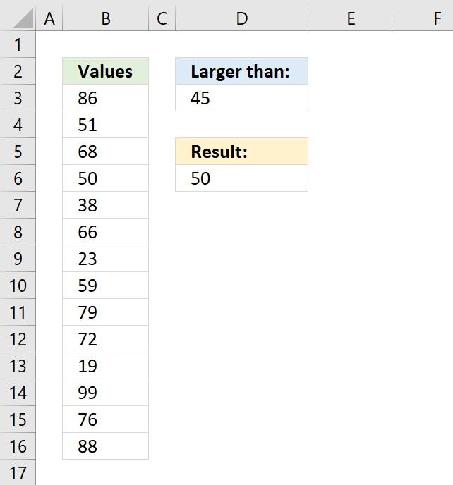
The example above specifies the given number in cell D3, in this case, 45. The data is in cell range B3:B16, the formula in cell D6 calculates the smallest value but larger than 45.
Table of Contents
-
- Find the smallest number that is larger than a given number - [Excel 2016]
- Find the smallest number that is larger than a given number - earlier Excel versions
- Find the largest number that is smaller than a given number - [Excel 2016]
- Find the largest number that is smaller than a given number - earlier Excel versions
- How to find the k-th smallest number that is larger than a given number?
- How to find the k-th largest number that is smaller than a given number?
- How to find the smallest number excluding zeros
- Get Excel file
15.1. Find the smallest number in a list that is larger than a given number - [Excel 2016]
This example shows an Excel 2016 function that extracts the smallest number larger than a given condition. The condition is specified in cell D3 and the source data is deployed in cell range B3:B16.
Cell D3 contains number 45, the formula in cell D6 returns 50 which is the smallest number larger than 45 in cell range B3:B16.
Formula in cell D6:
Section 2 below describes a formula that works in all Excel versions.
15.1.1 Explaining formula
Step 1 - Populate arguments
The MINIFS function calculates the smallest value based on a given set of criteria.
Function syntax: MINIFS(min_range, criteria_range1, criteria1, [criteria_range2, criteria2], ...)
MINIFS(min_range, criteria_range1, criteria1, [criteria_range2, criteria2], ...)
becomes
MINIFS(B3:B16,B3:B16,">"&D3)
The greater than sign > is a logical operator that lets you check if a number is larger than another number.
The ampersand character & lets you concatenate values in an Excel formula. You also have the option to enter the greater than sign in cell D3 combined with the given number, like this: >45. If you do remove the less than sign and the ampersand and reference only cell D3 in the MINIFS function.
Step 2 - Evaluate MINIFS function
MINIFS(B3:B16,B3:B16,">"&D3)
becomes
MINIFS({86; 51; 68; 50; ... ; 88},">"&45)
and returns 50.
15.2. Find the smallest number in a list that is larger than a number - earlier Excel versions
This example demonstrates a formula that works in all Excel versions, it extracts the smallest number larger than a given condition.
The condition is specified in cell D3 and the source data is in cell range B3:B16. Cell D3 contains number 45, the formula in cell D6 returns 50 which is the smallest number larger than 45 in cell range B3:B16.
Array formula in cell D6:
This formula is an array formula, it is required to enter this formula given the instructions in section 2.1 below if you work in an Excel version earlier than Excel 365.
15.2.1 How to enter an array formula
- Type the formula in cell B3
- Then press and hold CTRL and SHIFT simultaneously,
- Now press Enter once.
- Release all keys.
 The formula bar now shows the formula with a beginning and ending curly bracket telling you that you entered the formula successfully.
Don't enter the curly brackets yourself, they appear automatically.
Explaining array formula
Step 1 - Filter values in cell range larger than the condition in cell D3
The IF function allows you to create a logical expression that evaluates to TRUE or FALSE. You can then choose what will happen to a value that returns TRUE and also FALSE.
IF(logical_test, [value_if_true], [value_if_false])
If you use a cell range instead of a cell reference to a single cell you evaluate all the values in the cell range. The larger than sign lets you check if the values in B3:B16 are larger than the value in D3.
IF(B3:B16>D3,B3:B16)
returns the following array: {86;51;68;50;... ;88}
Step 2 - Return the smallest value in the array
The MIN function ignores boolean values which is useful in this case.
MIN(IF(B3:B16>D3,B3:B16)) returns 50 in cell D6.
15.3. Find the largest number in a list that is smaller than a given number - [Excel 2016]

The image above shows a small formula in cell D6 that calculates the largest number in cell range B3:B16 smaller than the condition specified in cell D3.
The formula in cell D6 returns 38, it is smaller than 45 but the largest of the numbers smaller than 45.
Excel 2016 formula in cell D6:
Section 4 describes a formula for earlier Excel versions than Excel 2016.
15.3.1 Explaining formula
Step 1 - Populate arguments
The MAXIFS function calculates the highest value based on a condition or criteria.
Function syntax: MAXIFS(max_range, criteria_range1, criteria1, [criteria_range2, criteria2], ...)
MIAXIFS(max_range, criteria_range1, criteria1, [criteria_range2, criteria2], ...)
becomes
MAXIFS(B3:B16,B3:B16,"<"&D3)
The less than sign < is a logical operator that lets you check if a number is smaller than another number. The ampersand character & lets you concatenate values in an Excel formula.
Step 2 - Evaluate MINIFS function
MINIFS(B3:B16,B3:B16,">"&D3)
becomes
MINIFS({86; 51; 68; 50; 38; ... ; 88},"<"&45)
and returns 38.
15.4. Find the largest number that is smaller than a given number - earlier Excel versions

Array formula in cell D6:
15.4.1 Explaining the formula
Step 1 - Filter values in cell range larger than the condition in cell D3
The IF function returns one value if the logical test is TRUE and another value if the logical test is FALSE.
Function syntax: IF(logical_test, [value_if_true], [value_if_false])
IF(B3:B16>D3,B3:B16)
becomes
IF({86;51;68;50;38;66;23;59;79;72;19;99;76;88}<45,B3:B16)
returns the following array: {FALSE;... ;38;FALSE;23; ... ;FALSE}
Step 2 - Return the smallest value in the array
The MAX function calculate the largest number in a cell range.
Function syntax: MAX(number1, [number2], ...)
MAX(IF(B3:B16>D3,B3:B16)) returns 38 in cell D6.
15.5. How to find the k-th smallest number that is larger than a given number?

Array formula in cell D6:
15.5.1 Explaining formula
Step 1 - Check if numbers are larger than the condition
The larger than character lets you preform logic in an Excel formula. The result is a boolean value TRUE or FALSE.
B3:B16>D3 returns {TRUE; TRUE; ... ; TRUE}.
Step 2 - Extract numbers larger than the condition in cell D3
The IF function returns one value if the logical test is TRUE and another value if the logical test is FALSE.
Function syntax: IF(logical_test, [value_if_true], [value_if_false])
IF(B3:B16>D3,B3:B16,"") returns {86; 51; ... ; 88}
Step 3 - Extract the k-th smallest number
The SMALL function returns the k-th smallest value from a group of numbers.
Function syntax: SMALL(array, k)
SMALL(IF(B3:B16>D3,B3:B16,""),D6) returns 51.
50 is the smallest number in the array, however, we are looking for the second smallest number in the array.
15.6. How to find the k-th largest number that is smaller than a given number?

Array formula in cell D6:
15.6.1 Explaining formula
Step 1 - check if numbers are smaller than the condition
B3:B16<D3 returns {FALSE; FALSE; ... ; FALSE}.
Step 2 - extract numbers smaller than the condition in cell D3
The IF function returns one value if the logical test is TRUE and another value if the logical test is FALSE.
Function syntax: IF(logical_test, [value_if_true], [value_if_false])
IF(B3:B16<D3,B3:B16,"") returns {""; ... ; 23; ... ; ""}.
Step 3 - extract the k-th largest number
The LARGE function calculates the k-th largest value from an array of numbers.
Function syntax: LARGE(array, k)
LARGE(IF(B3:B16<D3,B3:B16,""),D6) returns 23.
38 is the largest number in the array, however, we need to extract the second largest number specified in cell D6.
15.7. How to find the smallest number excluding zeros
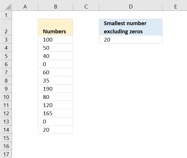
Column B contains numbers, the formula in cell D3 calculates the smallest value excluding zeros. Note that all numbers are either 0 (zero) or larger.
Formula in cell D3:
The MINIFS function appeared first in Excel 2016 and is a fairly new function. Here is the Excel function syntax:
MINIFS(min_range, criteria_range1, criteria1, [criteria_range2, criteria2], ...)
We only have one condition so the function syntax becomes:
MINIFS(min_range, criteria_range, criteria)
The min_range argument points to the cells containing the numbers B3:B14.
The criteria_range is the cell range to be evaluated B3:B14.
criteria is the condition, "<>0". <> means not equal to.
If cell in B3:B14 is not equal to 0 (zero) then return cell in B3:B14 and lastly find the smallest value.
Use the following array formula if you don't have access to the MINIFS function.
To enter an array formula, type the formula in a cell then press and hold CTRL + SHIFT simultaneously, now press Enter once. Release all keys.
The formula bar now shows the formula with a beginning and ending curly bracket telling you that you entered the formula successfully. Don't enter the curly brackets yourself.
Explaining formula in cell D3
Step 1 - Build logical expression
The IF function requires a logical expression in the first argument in order to return a given value when the logical expression evaluates to TRUE and another value when FALSE.
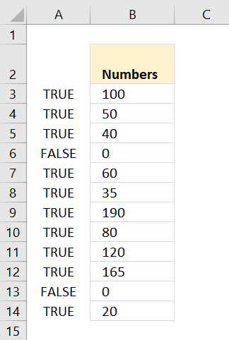 B3:B14<>0 returns {TRUE; TRUE; ... ; TRUE}.
I have entered the array in column A, note that boolean value FALSE corresponds to cells containing 0 (zero).
Step 2 - Filter values in array
The picture shows the array calculated by the IF function, each 0 (zero) is replaced with boolean value FALSE.
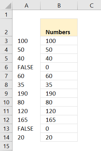 IF(B3:B14<>0, B3:B14)
returns {100; 50; 40; ... ; 20}
Step 3 - Find smallest value
The MIN function ignores text, blank and boolean values.
MIN(IF(B3:B14<>0,B3:B14)) returns 20 in cell D3.
16. Function not working
The SMALL function returns
- #VALUE! error if the second argument is a non-numeric input value.
- #NAME? error if you misspell the function name.
- propagates errors, meaning that if the input contains an error (e.g., #VALUE!, #REF!), the function will return the same error.
16.1 Troubleshooting the error value
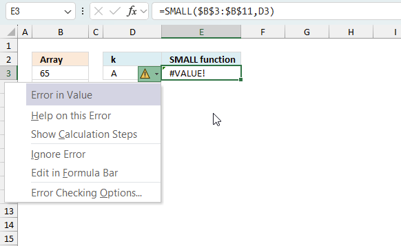
When you encounter an error value in a cell a warning symbol appears, displayed in the image above. Press with mouse on it to see a pop-up menu that lets you get more information about the error.
- The first line describes the error if you press with left mouse button on it.
- The second line opens a pane that explains the error in greater detail.
- The third line takes you to the "Evaluate Formula" tool, a dialog box appears allowing you to examine the formula in greater detail.
- This line lets you ignore the error value meaning the warning icon disappears, however, the error is still in the cell.
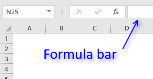
- The fifth line lets you edit the formula in the Formula bar.
- The sixth line opens the Excel settings so you can adjust the Error Checking Options.
Here are a few of the most common Excel errors you may encounter.
#NULL error - This error occurs most often if you by mistake use a space character in a formula where it shouldn't be. Excel interprets a space character as an intersection operator. If the ranges don't intersect an #NULL error is returned. The #NULL! error occurs when a formula attempts to calculate the intersection of two ranges that do not actually intersect. This can happen when the wrong range operator is used in the formula, or when the intersection operator (represented by a space character) is used between two ranges that do not overlap. To fix this error double check that the ranges referenced in the formula that use the intersection operator actually have cells in common.
#SPILL error - The #SPILL! error occurs only in version Excel 365 and is caused by a dynamic array being to large, meaning there are cells below and/or to the right that are not empty. This prevents the dynamic array formula expanding into new empty cells.
#DIV/0 error - This error happens if you try to divide a number by 0 (zero) or a value that equates to zero which is not possible mathematically.
#VALUE error - The #VALUE error occurs when a formula has a value that is of the wrong data type. Such as text where a number is expected or when dates are evaluated as text.
#REF error - The #REF error happens when a cell reference is invalid. This can happen if a cell is deleted that is referenced by a formula.
#NAME error - The #NAME error happens if you misspelled a function or a named range.
#NUM error - The #NUM error shows up when you try to use invalid numeric values in formulas, like square root of a negative number.
#N/A error - The #N/A error happens when a value is not available for a formula or found in a given cell range, for example in the VLOOKUP or MATCH functions.
#GETTING_DATA error - The #GETTING_DATA error shows while external sources are loading, this can indicate a delay in fetching the data or that the external source is unavailable right now.
16.2 The formula returns an unexpected value
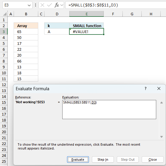
To understand why a formula returns an unexpected value we need to examine the calculations steps in detail. Luckily, Excel has a tool that is really handy in these situations. Here is how to troubleshoot a formula:
- Select the cell containing the formula you want to examine in detail.
- Go to tab “Formulas” on the ribbon.
- Press with left mouse button on "Evaluate Formula" button. A dialog box appears.
The formula appears in a white field inside the dialog box. Underlined expressions are calculations being processed in the next step. The italicized expression is the most recent result. The buttons at the bottom of the dialog box allows you to evaluate the formula in smaller calculations which you control. - Press with left mouse button on the "Evaluate" button located at the bottom of the dialog box to process the underlined expression.
- Repeat pressing the "Evaluate" button until you have seen all calculations step by step. This allows you to examine the formula in greater detail and hopefully find the culprit.
- Press "Close" button to dismiss the dialog box.
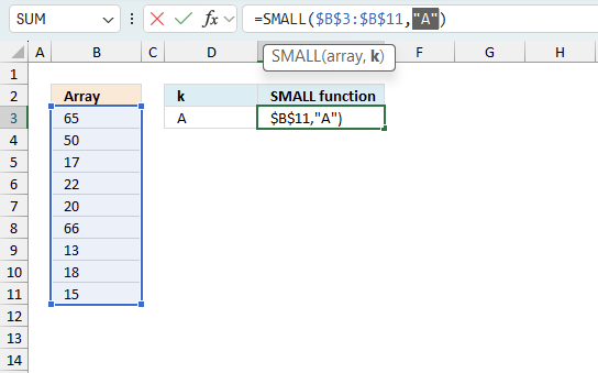
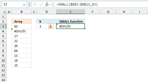
There is also another way to debug formulas using the function key F9. F9 is especially useful if you have a feeling that a specific part of the formula is the issue, this makes it faster than the "Evaluate Formula" tool since you don't need to go through all calculations to find the issue.
- Enter Edit mode: Double-press with left mouse button on the cell or press F2 to enter Edit mode for the formula.
- Select part of the formula: Highlight the specific part of the formula you want to evaluate. You can select and evaluate any part of the formula that could work as a standalone formula.
- Press F9: This will calculate and display the result of just that selected portion.
- Evaluate step-by-step: You can select and evaluate different parts of the formula to see intermediate results.
- Check for errors: This allows you to pinpoint which part of a complex formula may be causing an error.
The image above shows cell reference D3 converted to hard-coded value using the F9 key. The SMALL function requires numerical values which is not the case in this example. We have found what is wrong with the formula.
Tips!
- View actual values: Selecting a cell reference and pressing F9 will show the actual values in those cells.
- Exit safely: Press Esc to exit Edit mode without changing the formula. Don't press Enter, as that would replace the formula part with the calculated value.
- Full recalculation: Pressing F9 outside of Edit mode will recalculate all formulas in the workbook.
Remember to be careful not to accidentally overwrite parts of your formula when using F9. Always exit with Esc rather than Enter to preserve the original formula. However, if you make a mistake overwriting the formula it is not the end of the world. You can “undo” the action by pressing keyboard shortcut keys CTRL + z or pressing the “Undo” button
16.3 Other errors
Floating-point arithmetic may give inaccurate results in Excel - Article
Floating-point errors are usually very small, often beyond the 15th decimal place, and in most cases don't affect calculations significantly.
Useful links
How to find smallest positive value (greater than 0) in Excel?
Calculate the smallest or largest number in a range
Minimum Value in a Range if Greater Than "X"
'SMALL' function examples

This post explains how to lookup a value and return multiple values. No array formula required.

Array formulas allows you to do advanced calculations not possible with regular formulas.
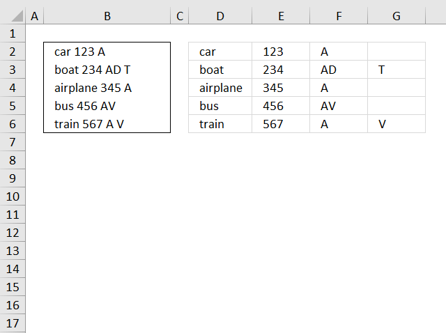
This blog article describes how to split strings in a cell with space as a delimiting character, like Text to […]
Functions in 'Statistical' category
The SMALL function function is one of 73 functions in the 'Statistical' category.
Excel function categories
Excel categories
12 Responses to “How to use the SMALL function”
Leave a Reply
How to comment
How to add a formula to your comment
<code>Insert your formula here.</code>
Convert less than and larger than signs
Use html character entities instead of less than and larger than signs.
< becomes < and > becomes >
How to add VBA code to your comment
[vb 1="vbnet" language=","]
Put your VBA code here.
[/vb]
How to add a picture to your comment:
Upload picture to postimage.org or imgur
Paste image link to your comment.
Hi Oscar,
I am in love with.. your formula explanation.. :)
Waiting eagerly for MMULT & some D-Functions..
Regards,
Deb
Debraj Roy,
Thank you!
I am curious, in what situation do you use MMULT?
Hi Oscar,
We can use MMULT in all cases where SUMPRODUCT fails..
with only Two Criteria..
* Only TWO Array can be multiplied..
* 1st Array's No Of Row.. Should be Same as 2nd Array's No Of Column..
Unlike SUMPRODUCT, It returns ARRAY output..
I think, Binary Addition & Binary Multiplication are the base of all FORMULA's & FUNCTION..
and you are doing a great job, by teaching/using them in your daily blog..
Regards!
Deb
Debraj Roy,
Well, I am learning from you right now.
Can you provide an example where SUMPRODUCT fails and MMULT succeeds?
I searched and found my old mathematics books from college, I had forgotten the basics of multiplying two matrices. :-)
It is worthwhile mentioning that in both Small and Large K could also be an array
So if A1:A10 contains random numbers the below formulas
=Large(A1:A10,{1,2,3}) - Return an array containing the top 3 numbers
=SUM(Large(A1:A10,{1,2,3}) -Array entered Returns the Sum of the top 3 numbers
=SUM(LARGE(A1:A10,ROW(INDIRECT("1:"&TopN))))- Array Entered Returns the sum of the Top N numbers as defined in the Cell/Named Constant TopN
=Large(A1:A10,Row(A1:A10))- Array entered returns an array of numbers in A1:A10 in Descending order
Likewise Small
sam,
It is worthwhile mentioning that in both Small and Large K could also be an array
Yes you are right! Thanks for pointing that out.
=Small({VALUE(DV147),VALUE(DZ147),VALUE(ED147),VALUE(EH147)},2) will not work. If I use sum and the "Value(-----)" amounts, it works.
What am I doing wrong?
The numbers are stored as text in those cells for other reasons.
I'm using the SMALL function inside an array. I understand how to use the function to return an array where values are greater than or equal to a number. But how do I use the function if I want to return results that are between two numbers?
I've tried nesting an AND statement within the IF statement, but it isn't working (no values are returned).
Any suggestions? Thanks!
julie,
=SMALL(IF(($A$2:$A$10<$F$2)*($A$2:$A$10>$F$3),$A$2:$A$10,""),ROW(A1))
Hi,
Is there a way to do this same idea, but when your data is organized vertically? You appear to be the only person that I've seen solve my problem - which is, bring back all results based upon a specific date AND sort that data dynamically (smallest number to largest) in a separate tab without having to adjust the sorting manually. I've tried out your file and tried to adjust the formula for my purposes, but am missing something when I do.
Report Tab:
N3 = My manually entered date field to match to
A6 = The first field where the formula & smallest results would go (Then A7, etc).
Data Tab: Fields may contain data, be empty and/or contain a formula
Column C = Date field to compare with N3 (Named range of ArrivalDate (C3 to C500))
Column A = Number to sort by. (Named range of SortCode (A3 to A500))
I've got it working today based upon the smallest row number being returned, but really want it based upon the small value first.
My formula now is: =IFERROR(INDEX(SortCode,SMALL(IF(ArrivalDate=$N$3,ROW(SortCode)),ROW(1:1))-1,),"")
Any suggestions/help are welcome. My first time using Index functionality.
Thank you so much!
Todd
Todd,
try this array formula:
=IFERROR(INDEX(SortCode,MATCH(SMALL(IF(ArrivalDate=$N$3,SortCode),ROWS($A$1:A1)),SortCode,0)),"")
very interesting