How to use the FREQUENCY function
What is the FREQUENCY function?
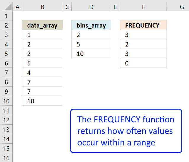
The FREQUENCY function calculates how often values occur within a range of values (interval) and returns a vertical array of numbers. It returns an array that is one more item larger than the bins_array.
Table of contents
- Introduction
- Syntax
- Arguments
- Example
- Working with a condition
- 3d ranges
- Frequency bug?
- Count unique distinct numbers across multiple sheets
- Get Excel file
- Sum numerical ranges between two numbers
- Sort column based on count
- Sort rows based on count and criteria - Excel 365
- Sort rows based on count and criteria - earlier versions
1. Introduction
What is the absolute frequency?
The absolute frequency is the number of times a specific value or data point appears in a given dataset. It represents the total number of occurrences of each distinct value or category within the dataset. Absolute frequency is also known as the raw frequency or frequency count.
Let's consider an example of exam scores: 65, 82, 86, 91, 65, 82, 86, 94.
Absolute Frequency:
Score 65: 2
Score 82: 2
Score 86: 2
Score 91: 1
Score 94: 1
What is the absolute cumulative frequency?
The absolute cumulative frequency is the running total or accumulation of the absolute frequencies up to a particular value or category in a dataset. It is calculated by adding the absolute frequencies of all the values or categories that are less than or equal to the current value or category.
Score 65: absolute cumulative frequency: 2
Score 82: absolute cumulative frequency: 4 (2+2)
Score 86: absolute cumulative frequency: 6 (2+2+2)
Score 91: absolute cumulative frequency: 7 (2+2+2+1
Score 94: absolute cumulative frequency: 8 (2+2+2+1+1)
What is the relative frequency?
The relative frequency, also known as the frequency ratio or proportion, is the fraction or percentage of times a specific value or category occurs in a dataset. It is calculated by dividing the absolute frequency of a particular value or category by the total number of data points in the dataset.
Score 65: 2/8 = 0.25 or 25%
Score 82: 2/8 = 0.25 or 25%
Score 86: 2/8 = 0.25 or 25%
Score 91: 1/8 = 0.125 or 12.5%
Score 94: 1/8 = 0.125 or 12.5%
The total is 100% (25+25+25+12.5+12.5 = 100)
What is the cumulative relative frequency?
The cumulative relative frequency is the running total or accumulation of the relative frequencies up to a particular value or category in a dataset. It is calculated by adding the relative frequencies of all the values or categories that are less than or equal to the current value or category.
Score 65: 2/8 = 0.25 or 25%
Score 82: 4/8 = 0.5 or 50% (25+25)
Score 86: 6/8 = 0.75 or 75% (25+25+25)
Score 91: 7/8 = 0.875 or 87.5% (25+25+25 +12.5)
Score 94: 8/8 = 1 or 100% (25+25+25 +12.5+12.5)
2. Syntax
FREQUENCY(data_array, bins_array)
3. Arguments
| data_array | An array or cell range for which you want to determine frequencies. |
| bins_array | The intervals which you want to group the values in. |
The FREQUENCY function returns two or more values in a vertical array, blank cells and text strings are ignored. This means that you can only use the function with numerical values.
4. Example 1

You have a dataset of exam scores ranging from 0 to 100. Use the FREQUENCY function to calculate the number of students who scored within different score ranges?
The image above shows the exam scores in cell range B18:F22. Here are the exam scores:
| 59 | 50 | 38 | 12 | 37 |
| 75 | 79 | 29 | 59 | 25 |
| 80 | 48 | 51 | 70 | 95 |
| 95 | 98 | 52 | 15 | 39 |
| 38 | 1 | 21 | 90 | 16 |
Cell range B25:B34 contains the intervals displayed in the histogram chart below the columns. Cell range C25:C34 contains the intervals the FREQUENCY function uses to calculate how often values occur within the specified range of values.
Array formula in cell D25:
The formula in returns an array of values: {1;3;3;4;2;4;1;3;1;3;0} These numbers are the frequency or count based on the intervals specified in cell range C25:C34.
Note that the array is one value larger than the number of cells in C25:C34. The last value in the array corresponds to values larger than the last interval value, in this example 100. 0 (zero) means that there are no values larger than 100.
The numbers in {1;3;3;4;2;4;1;3;1;3;0} correspond the the intervals in C25:C34, for example the first value 1 in the array correspond to the first interval which is 10 meaning values smaller than or equal to 10. Only number 1 in B18:F22 is smaller or equal to 10.
The formula is an array formula and must be entered as an array formula if you use an Excel version earlier than Excel 365. Excel 365 subscribers can enter the formula as a regular formula simply by pressing Enter.
4.1 How to enter an array formula
Skip these steps if you are an Excel 365 subscriber.
- Select cell range D25:D35
- Type the formula.
- Press and hold CTRL + SHIFT keys simultaneously.
- Press Enter once. Release all keyboard keys.
The formula will now begin and end with a curly bracket, like this: {=array_formula}
They appear automatically, do not enter these characters yourself.
5. Example 2

You are a researcher studying a specific phenomenon, and you have collected data that falls into two distinct categories. However, to begin your analysis, you only need to focus on one of the categories for now. Your task is to calculate the frequency distribution for the data points within this single category, ignoring the other category for the time being.
The first category is labeled "A" and the second category "B", calculate the frequency distribution of category "A"?
The data is in cell range B17:C32 shown in the image above. Here is the data:
| Item | Value |
| A | 1 |
| B | 2 |
| A | 2 |
| B | 5 |
| A | 4 |
| B | 7 |
| A | 7 |
| B | 10 |
| A | 1 |
| B | 4 |
| A | 4 |
| B | 9 |
| A | 4 |
| B | 7 |
| A | 7 |
| B | 9 |
The image above shows the FREQUENCY function entered in F17 using an IF function to filter values based on a condition.
Array formula in cell range F17:
The following formula calculates the unique distinct numbers based on category "A". Excel 365 dynamic array formula in cell E17:
This formula spills values to cell E17 and cells below as far as needed. For example, category "B" contains value 9 which category "A" does not have. Value 9 is not present in the list in E17 and cells below, only values in category "A".
The image above shows the distribution in cell E17 and cells below, the corresponding frequency in cell F17 and cells below. Above the distribution is a histogram chart showing the distribution and the frequency.
5.1 Explaining the calculation
I recommend using the "Evaluate Formula" feature to learn more about formulas. This tool allows you to examine formula calculations in detail. It also lets you troubleshoot formulas, what is making my formula return an error?
Go to tab "Formulas" on the ribbon and press with left mouse button on the "Evaluate Formula" button. A dialog box appears, press with left mouse button on the "Evaluate" button to move to the next step in formula calculation. Press with left mouse button on "Close" button to dismiss the dialog box.
Step 1 - Filter values
The IF function lets you return a value if a logical expression returns TRUE and another value if FALSE, the logical expression usually returns a boolean value but their equivalents work just fine. FALSE -> 0 (zero), TRUE -> any number.
IF(B17:B32="A",C17:C32,"")
We want to compare the values in cell range B3:B10 with "A" and if they match then return the corresponding value on the same row in cell range C3:C10. IF no match return a blank "".
IF(B17:B32="A",C17:C32,"")
becomes
IF({"A";"B";"A";... ;"B"}="A",{1;2;2;...;9},"")
becomes
IF({TRUE;FALSE;TRUE;...;FALSE},{1;2;2;...;9},"")
and returns this array: {1;"";2;"";4;"";7;"";1;"";4;"";4;"";7;""}.
Step 2 - Frequency
The FREQUENCY function uses the array from the IF function in the first argument, blank values "" are ignored.
FREQUENCY(IF(B3:B10="A",C3:C10,""),E17#)
becomes
FREQUENCY({1;"";2;"";4;"";7;"";1;"";4;"";4;"";7;""},E17#)
becomes
FREQUENCY({1; ""; 2; ""; 4; ""; 7; ""},{1;2;4;7})
and returns {2;1;3;2;0} in cell range F17 and cells below.
6. 3D ranges

You are a scientist and have gathered data across multiple worksheets, how do you calculate the frequency distribution based on multiple worksheets (3D ranges)? Your data is in cell range B3:B10 on two worksheets named '3D range' and '3D range1'
This example demonstrates how to use the FREQUENCY function with 3D references. 3D ranges are cell ranges across worksheets meaning a cell reference to a specified number of worksheets in a workbook. Section 6.1 describes how to enter a 3D range.
Array formula in cell D3:
The image above shows the combined frequency distribution in cell range D3:D11 from worksheets '3D range' and '3D range1' based on the numbers specified in cell B3:B10.
This lets you work with data from multiple worksheets using the FREQUENCY function, I will now show you how to enter a 3D range using the FREQUENCY function.
Other Excel functions that can work with 3D ranges are SUM, AVERAGE, AVERAGEA, COUNT, COUNTA, MAX, MAXA, MIN, MINA, PRODUCT, STDEV, STDEVA, STDEVP, STDEVPA, VAR, VARA, VARP, VARPA functions
6.1 How to enter a formula containing 3D ranges
The formula contains a 3-D reference to a range of worksheet names, make sure you rearrange the worksheets so only worksheets you want to include are being used.
- Select cell range D3:D10.
- Press with left mouse button on in the formula bar, the prompt appears.
- Type =FREQUENCY(
- Press and hold SHIFT key.
- Select the last worksheet you want to include in the FREQUENCY function.
- Release SHIFT key.
- Select cell range B3:B10 with the mouse.
- Type , (comma)
- Select cell range B3:B10 with the mouse.
- Now enter the formula as an array formula (Excel 365 users can skip this step and simply press Enter).
- Here are the steps sto enter an array formula.
- Press and hold CTRL + SHIFT keys simultaneously.
- Press Enter once.
- Release all keys.
The formula has now a leading and trailing curly bracket, like this: {=array_formula]
Don't enter these characters yourself, they appear automatically. The image above does not show these characters because I use Excel 365 which uses dynamic array formulas that automatically spill values to cells below.
6.2 How to rearrange worksheets

The image above shows three worksheet names, "3D range", "Sheet7", and "3D range1". We want to move worksheet "Sheet7" so it is not included in the FREQUENCY function.
- Press and hold with mouse on worksheet name "Sheet7".
- Drag with mouse to move the worksheet tab to a new location.
- Release the mouse button to release the worksheet tab.

The image above shows "Sheet7" in a new location, you can now create a 3D reference to worksheets "3D range" and "3D range1".
7. Frequency bug?
Can someone explain to me why this happens?
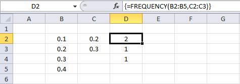
The example above is working.
FREQUENCY function returns {2; 1; 1}. 2 values (0.1 and 0.2) are equal to or less than 0.2. 1 value (0.3) is larger than 0.2 and equal or smaller than 0.3. 1 value (0.4) is larger than 0.3.
The example below is not working as I thought it would.
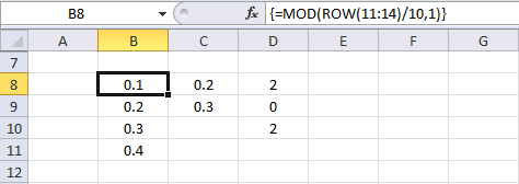
FREQUENCY function returns {2; 0; 2} and I don't understand why?
The formula in cell B8:B11 returns this array {0.1; 0.2; 0.3; 0.4}, exactly the same values as in B2:B5.
It seems to be the MOD function but why?
Why am I using the MOD function?
To extract the fractional part of a number.
Get workbook
8. Count unique distinct numbers across multiple sheets

I demonstrated in section 6 that the FREQUENCY function is able to calculate the frequency of given numbers across multiple worksheets or 3D ranges. This technique makes it possible to count unique distinct numbers across multiple worksheets as well.
Note that it is only possible with numerical values, not text values or other values which is quite limiting. However, the new VSTACK and UNIQUE functions makes it possible regardless of value types and without any issues. However, you need Excel 365.
The image above demonstrates three different formulas in column E that
- counts unique numbers (section 8.1)
- counts unique distinct numbers (section 8.2)
- counts duplicate numbers (section 8.3)
from multiple sheets in the same workbook.
8.1 Count unique distinct numbers
The following formula counts unique distinct numbers in multiple sheets (3D range):
Formula in E8:
To enter an array formula, type the formula in a cell then press and hold CTRL + SHIFT simultaneously, now press Enter once. Release all keys.
The formula bar now shows the formula with a beginning and ending curly bracket telling you that you entered the formula successfully. Don't enter the curly brackets yourself.
Explaining formula in cell E8
Step 1 - Count numbers
The FREQUENCY function calculates the number of times a number exists in a cell range, it also has the ability to count numbers across multiple worksheets.

The FREQUENCY function returns the count for the corresponding number only once. Example, 3 exists twice in column B above so the function returns 2 on the same row, however, the next time 3 appears in the list the function returns 0 (zero), see row 8. We can use that to count numbers.
FREQUENCY(Sheet1:Sheet3!$B$2:$D$4, Sheet1:Sheet3!$B$2:$D$4)
returns
{1; 9; 7; 0; 0; 0; 0; 0; 0; 0; 8; 0; 0; 1; 0; 0; 0; 0; 0; 0; 0; 0; 1; 0; 0; 0; 0; 0}.
Step 2 - Check if number in array is not equal to 0 (zero)
The less and greater than sign together means not equal to.
FREQUENCY(Sheet1:Sheet3!$B$2:$D$4, Sheet1:Sheet3!$B$2:$D$4)<>0
becomes
{1; 9; 7; ... ; 0}<>0
and returns
{TRUE; TRUE; ... ; FALSE}.
Step 3 - Convert boolean values to numerical equivalents
The SUMPRODUCT function can't sum boolean values so we need to convert TRUE to 1 and FALSE to 0 (zero). There are a few ways to convert them, you can add a zero or multiply with 1 or in this example use double negatives.
--(FREQUENCY(Sheet1:Sheet3!$B$2:$D$4, Sheet1:Sheet3!$B$2:$D$4)<>0)
returns {1; 1; 1; 0; 0; 0; 0; 0; 0; 0; 1; 0; 0; 1; 0; 0; 0; 0; 0; 0; 0; 0; 1; 0; 0; 0; 0; 0}.
Step 4 - Add numbers in array
SUMPRODUCT(--(FREQUENCY(Sheet1:Sheet3!$B$2:$D$4, Sheet1:Sheet3!$B$2:$D$4)<>0))
becomes
SUMPRODUCT({1; 1; 1; 0; 0; 0; 0; 0; 0; 0; 1; 0; 0; 1; 0; 0; 0; 0; 0; 0; 0; 0; 1; 0; 0; 0; 0; 0})
and returns 6.
8.2 Count unique numbers
This formula counts unique numbers in multiple sheets (3D range)
Formula in E10:
8.3 Count duplicate numbers
Formula in E12:
Get excel tutorial file
Count unique and duplicate numerical data entries from multiple sheets.xls
(Excel 97-2003 Workbook *.xls)
9. Excel file
10. Sum numerical ranges between two numbers

This article explains how to build an array formula that sums numerical ranges. Example, I want to know how to calculate the total sum between x.2 -x.3 and x.5-x.8, and the range is 0.5 and 4.5.
Why is this useful? Excel date and time values are numerical values formatted as date/time. The last section demonstrates how to calculate a total based on time ranges and a start/end date/time.
What's on this webpage
- How to manually sum ranges
- How to sum ranges in Excel
- How to sum time across days with a start and end time each day
- Get Excel file
10.1. How to manually sum ranges

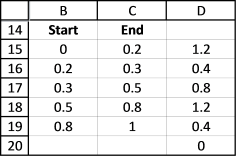
This picture shows you how to manually sum the ranges x.2-x.3 and x.5-x.8 between 0.5 and 4.5.
The range starts at 0.5 so 0.2-0.3 is 0. 0.5-0.8 is 0.3. Total sum between 0.5-1 is 0.3.
1.2-1.3 is 0.1 and 1.5-1.8 is 0.3. The total between 1-2 is 0.4.
2.2-2.3 is 0.1 and 2.5-2.8 is 0.3. The total between 2-3 is 0.4.
3.2-3.3 is 0.1 and 3.5-3.8 is 0.3. The total between 3-4 is 0.4.
4.2-4.3 is 0.1 and 4.5-4.8 is 0 because the range ends at 4.5. The total between 4-4.5 is 0.1.
![]()
The grand total is 1.6 (0.3+0.4+0.4+0.4+0.4+0.1 = 1.6).
10.2. How to sum ranges in Excel

The image above shows how to calculate overlapping numerical ranges. Cell C3 shows the start of the range and cell D3 shows the end point of the numerical range. In this example, the start is at 0.5 and the end is at 4.5.
There are two overlapping ranges, they are at x.1 to x.3 and x.5 to x.8. The x means that they are valid for any number, for example 0.1 to 0.3 but also 1.1 to 1.3 etc. The formula in cell F21 calculates the total of the overlapping ranges based on the start number and the end number in cells C3:D3.
Cell range B6:E12 shows the manual calculation for each overlapping range and the total, I demonstrated this in section 10.1 above.
Cell range B14:F21 shows how the formula works by displaying the totals row by row. This formula, presented here, works only with ranges that has one decimal, here is a formula that works with all kinds of numerical ranges: Calculate machine utilization
Array formula in cell F21:
Step 1 - Create cell reference
The INDEX function is able to create a cell reference that can be used to create an array. This technique is better than using the INDIRECT function which is volatile.
INDEX($A:$A, (D3-C3)*10)
becomes
INDEX($A:$A, (4.5-0.5)*10)
becomes
INDEX($A:$A, 4*10)
becomes
INDEX($A:$A, 40)
and returns A40
Step 2 - Create a cell reference to a cell range
You can concatenate the output from the INDEX function with another cell reference so that it points to a cell range. Weirdly, you don't need to use the ampersand character or double quotations to do so. This is the only case that I know of when this is possible.
$A$1:INDEX($A:$A, (D3-C3)*10)
becomes
$A$1:A40
Step 3 - Create an array based on a cell reference
The ROW function returns a number representing the row number from a cell reference. The ROW function returns an array of row numbers ff the cell reference points to a cell range.
ROW($A$1:INDEX($A:$A, (D3-C3)*10))
becomes
ROW($A$1:A40)
and returns {1; 2; 3; 4; 5; 6; 7; 8; 9; 10; 11; 12; 13; 14; 15; 16; 17; 18; 19; 20; 21; 22; 23; 24; 25; 26; 27; 28; 29; 30; 31; 32; 33; 34; 35; 36; 37; 38; 39; 40}
Step 4 - Divide by 10
ROW($A$1:INDEX($A:$A, (D3-C3)*10))/10
becomes
{1; 2; 3; 4; 5; 6; 7; 8; 9; 10; 11; 12; 13; 14; 15; 16; 17; 18; 19; 20; 21; 22; 23; 24; 25; 26; 27; 28; 29; 30; 31; 32; 33; 34; 35; 36; 37; 38; 39; 40}/10
and returns
{0.1; 0.2; 0.3; 0.4; 0.5; 0.6; 0.7; 0.8; 0.9; 1; 1.1; 1.2; 1.3; 1.4; 1.5; 1.6; 1.7; 1.8; 1.9; 2; 2.1; 2.2; 2.3; 2.4; 2.5; 2.6; 2.7; 2.8; 2.9; 3; 3.1; 3.2; 3.3; 3.4; 3.5; 3.6; 3.7; 3.8; 3.9; 4}
Step 5 - Create a sequence
C3+ROW($A$1:INDEX($A:$A, (D3-C3)*10))/10
becomes
C3+{0.1; 0.2; 0.3; 0.4; 0.5; 0.6; 0.7; 0.8; 0.9; 1; 1.1; 1.2; 1.3; 1.4; 1.5; 1.6; 1.7; 1.8; 1.9; 2; 2.1; 2.2; 2.3; 2.4; 2.5; 2.6; 2.7; 2.8; 2.9; 3; 3.1; 3.2; 3.3; 3.4; 3.5; 3.6; 3.7; 3.8; 3.9; 4}
becomes
0.5+{0.1; 0.2; 0.3; 0.4; 0.5; 0.6; 0.7; 0.8; 0.9; 1; 1.1; 1.2; 1.3; 1.4; 1.5; 1.6; 1.7; 1.8; 1.9; 2; 2.1; 2.2; 2.3; 2.4; 2.5; 2.6; 2.7; 2.8; 2.9; 3; 3.1; 3.2; 3.3; 3.4; 3.5; 3.6; 3.7; 3.8; 3.9; 4}
and returns
{0.6; 0.7; 0.8; 0.9; 1; 1.1; 1.2; 1.3; 1.4; 1.5; 1.6; 1.7; 1.8; 1.9; 2; 2.1; 2.2; 2.3; 2.4; 2.5; 2.6; 2.7; 2.8; 2.9; 3; 3.1; 3.2; 3.3; 3.4; 3.5; 3.6; 3.7; 3.8; 3.9; 4; 4.1; 4.2; 4.3; 4.4; 4.5}
Step 6 - Filter decimals from number
We only need the decimal part of the values in this array.
MOD(C3+ROW($A$1:INDEX($A:$A, (D3-C3)*10))/10, 1)
becomes
MOD({0.6; 0.7; 0.8; ... ; 4.3; 4.4; 4.5}, 1)
and returns
{0.6;0.7;0.8; ... ;0.2;0.3;0.4;0.5}
Step 7 - Workaround for floating point error
ROUND(MOD(C3+ROW($A$1:INDEX($A:$A, (D3-C3)*10))/10, 1), 1)
ROUND({0.6;0.7;0.8; ... ;0.2;0.3;0.4;0.5}, 1)
and returns {0.6; 0.7; ... 0.3; 0.4; 0.5}.
The MOD function returns the decimal part of a number, unfortunately, it returns a floating point error. The ROUND function takes care of that.
Step 8 - Evaluate FREQUENCY function
The second task is to build the ranges. We are going to use the FREQUENCY function and therefore we need to be more specific regarding the ranges.
The picture shows not only 0.2-0.3 and 0.5-0.8 but also other ranges before, between, and after. We are not interested in those ranges but they are required in order to get the FREQUENCY function to work as we want.
It is now time to use the frequency function with our array and our ranges:
The array formula returns an array shown in D15:D20. The range we are using is 0.5 to 4.5, remember? 4.5 - 0.5 is 4. 4 is supposed to be equal to the sum of the frequency values in D15:D20. Lets verify that, 1.2+0.4+0.8+1.2+0.4 = 4. Correct.
Step 9 - Multiply arrays
The third task is to sum the ranges we need. In order to do that I have built a new column "Count", 1 for a range I want in the sum and 0 for a range I don´t want.
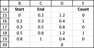
Lets multiply the array formula with the "Count" column (E15:E19):
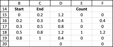
This formula returns {0; 0.4; 0; 1.2; 0; 0}.
Step 10 - Add numbers and return total
Then use the SUM function to sum the values in the array:
returns 1.6. 0.4 + 1.2 is 1.6, it matches the manual calculation we did in the beginning of this blog post.
Why would you want to sum numerical ranges? Consider that date and time values are actually numbers in excel, get it? Read the next section below.
10.3. How to sum time based on time periods across days

The array formula in cell C9 is adapted to counting minutes, it compares the time range based on the values in cell C2 and C3 (start and end date/time) to the time ranges in the Excel Table (cell range B6:C7) and adds the minutes that fall between the time ranges.
You can easily add more time ranges to the Excel Table without adjusting the formula. There are two structured references that point to the Excel Table, Table1[Column1] and Table1[Time ranges].
The array formula in cell C9 recalculates if you change the start/end value in C2,C3 or add/delete/edit the time ranges in B6:C7. Note that there is a limit to the size of the start and end date, the formula won't work if the range is larger than 728,18 days. This is because the array size in Excel formulas is limited to 1048576 values.
Array formula in cell C9:
Excel 365 formula in cell C9
11. Sort column based on count

This section demonstrates a formula that sorts cell values by their frequency, in other words, how many times a value is repeated in the list.
Table of Contents
11.1. Sort column based on the count
Question:
How do I create a new unique distinct list from a column? I also want the list sorted from large to small by the number of times a value is repeated?
Answer:
Array formula in cell D3:
11.1.1 How to create an array formula
- Copy (Ctrl + c) and paste (Ctrl + v) array formula into formula bar. See the picture below.
- Press and hold Ctrl + Shift.
- Press Enter once.
- Release all keys.

Recommended article
Recommended articles

Array formulas allows you to do advanced calculations not possible with regular formulas.
How to copy array formula in cell D3
- Select cell D3
- Copy cell (Ctrl + c)
- Select cell range D4:D8
- Paste (Ctrl + v)
11.1.2 Explaining array formula in cell D3
Step 1 - Count previous items
The COUNTIF function calculates the number of cells that is equal to a condition.
COUNTIF(range, criteria)
COUNTIF($D$2:D2, B3:B14)
returns {0; ... ; 0}.
Step 2 - Identify positions of previous items
The equal sign compares each value in the array to 0 (zero), the result is a boolean value TRUE or FALSE.
COUNTIF($D$2:D2, B3:B14)=0
returns {TRUE; ... ; TRUE}.
Step 3 - Count items in the list
COUNTIF(B3:B14, B3:B14)
returns {2; 4; 4; 2; 4; 2; 3; 4; 2; 3; 1; 3}.
Step 4 - Create array containing count for new values
The IF function returns one value if the logical test is TRUE and another value if the logical test is FALSE.
IF(logical_test, [value_if_true], [value_if_false])
IF(COUNTIF($D$2:D2, B3:B14)=0, COUNTIF(B3:B14, B3:B14), "")
returns {2; 4; 4; 2; 4; 2; 3; 4; 2; 3; 1; 3}.
Step 5 - Get largest count
The LARGE function calculates the k-th largest value from an array of numbers.
LARGE(array, k)
LARGE(IF(COUNTIF($D$2:D2, B3:B14)=0, COUNTIF(B3:B14, B3:B14), ""), 1)
becomes
LARGE({2; 4; 4; 2; 4; 2; 3; 4; 2; 3; 1; 3}, 1)
and returns 4.
Step 5 - Find the position in the array of the largest count
The MATCH function returns the relative position of an item in an array or cell reference that matches a specified value in a specific order.
MATCH(lookup_value, lookup_array, [match_type])
MATCH(LARGE(IF(COUNTIF($D$2:D2, B3:B14)=0, COUNTIF(B3:B14, B3:B14), ""), 1), COUNTIF(B3:B14, B3:B14)*(COUNTIF($D$2:D2, B3:B14)=0), 0)
becomes MATCH(4, {2; 4; 4; 2; 4; 2; 3; 4; 2; 3; 1; 3}), 0) and returns 2.
Step 6 - Get value based on position
The INDEX function returns a value from a cell range, you specify which value based on a row and column number.
INDEX(array, [row_num], [column_num], [area_num])
INDEX(B3:B14, MATCH(LARGE(IF(COUNTIF($D$2:D2, B3:B14)=0, COUNTIF(B3:B14, B3:B14), ""), 1), COUNTIF(B3:B14, B3:B14)*(COUNTIF($D$2:D2, B3:B14)=0), 0))
returns "AA" in cell D3.
The following formula returns the count of the corresponding value in column D.
Formula in E3:
=COUNTIF($B$3:$B$14, D3)
Recommended articles

Counts the number of cells that meet a specific condition.
11.2. Sort column by count - Excel 365

The formula in cell D3 extracts unique distinct values from B3:B14 and returns a sorted list based on the number of instances of each value.
Excel 365 dynamic array formula in cell D3:
11.2.1 Explaining formula in cell D3
Step 1 - Count each value
The COUNTIF function calculates the number of cells that is equal to a condition.
COUNTIF(range, criteria)
COUNTIF(B3:B14, B3:B14)
returns {2; 4; 4; 2; 4; 2; 3; 4; 2; 3; 1; 3}.
Step 2 - Sort values by count
The SORTBY function allows you to sort values from a cell range or array based on a corresponding cell range or array. It sorts values by column but keeps rows.
SORTBY(array, by_array1, [sort_order1], [by_array2, sort_order2], …)
SORTBY(B3:B14, COUNTIF(B3:B14, B3:B14), -1)
returns
{"AA"; "AA"; "AA"; "AA"; "EE"; "EE"; "EE"; "DD"; "BB"; "DD"; "BB"; "CC"}.
Step 3 - Filter unique distinct values
The UNIQUE function extracts unique distinct rows from the array.
UNIQUE(array,[by_col],[exactly_once])
UNIQUE(SORTBY(B3:B14, COUNTIF(B3:B14, B3:B14), -1))
returns {"AA"; "EE"; "DD"; "BB"; "CC"}.
11.3. Get Excel Example File
12. Sort rows based on count and criteria - Excel 365
Andre asks:I am trying to list people with the highest scores based on certain criteria.
My data:
column
A B C D
Mike 207 Yes Life
Greg 207 Yes Life
Sid 207 Yes Life
Greg 207 Yes Life
Greg 207 Yes Life
Sid 207 Yes Life
Greg 207 No Life
Sid 204 No Health
criteria
countif b= 207 and column c= yes and column d= Life
and it then needs to arrange it from the highest to the lowest
(Large)
and then match it with the name eg, Greg Sid or Mike
so what I am looking for is eg.
Greg 3
Sid 2
Mike 1
but it has to be in one formula.

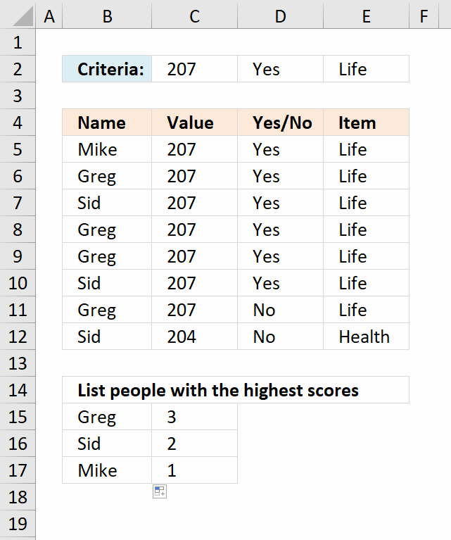
The formula counts the number of rows that meet all criteria specified in row 2. It then returns a list of names that are sorted by how often they appear in the rows that match the criteria.
The data set is in B5:E12, the criteria is specified in cells C2, D2, and E2. The formula uses the criteria and the names in B5:B12 to count rows meeting the criteria.
For example, all rows except row 11 and 12 meet the criteria. Mike (row 5) exists only once, Greg (row 6) exists three times, the other rows are 8 and 9. Note that Greg is in row 11 as well, however, the adjacent values do not meet the criteria specified in row 2.
Sid has three rows, however, only two rows meet the criteria and they are row 7 and 10.
Excel 365 formula in cell B15:
This is an Excel 365 dynamic array formula that spills values to cells below and to the right, enter this formula as a regular formula.
Update! New Excel 365 function - GROUPBY function
Excel 365 dynamic array formula in cell B15:
=GROUPBY(B5:E12,E5:E12,COUNTA,0,0,-5,(C5:C12=C2)*(D5:D12=D2)*(E5:E12=E2))
Explaining formula
Step 1 - List unique distinct items
[insertunc id="UNIQUE"]
UNIQUE(B5:B12)
becomes
UNIQUE({"Mike";"Greg";"Sid";"Greg";"Greg";"Sid";"Greg";"Sid"})
and returns
{"Mike";"Greg";"Sid"}
Step 2 - Count rows based on criteria and item
The COUNTIFS function calculates the number of cells across multiple ranges that equals all given conditions.
Function syntax: COUNTIFS(criteria_range1, criteria1, [criteria_range2, criteria2]…)
COUNTIFS(B5:B12,UNIQUE(B5:B12),C5:C12,C2,D5:D12,D2,E5:E12,E2)
becomes
COUNTIFS({"Mike";"Greg";"Sid";"Greg";"Greg";"Sid";"Greg";"Sid"},{"Mike";"Greg";"Sid"},{207;207;207;207;207;207;207;204},207,{"Yes";"Yes";"Yes";"Yes";"Yes";"Yes";"No";"No"},"Yes",{"Life";"Life";"Life";"Life";"Life";"Life";"Life";"Health"},"Life")
and returns
{1;3;2}
Step 3 - Add arrays horizontally
The HSTACK function combines cell ranges or arrays. Joins data to the first blank cell to the right of a cell range or array (horizontal stacking)
Function syntax: HSTACK(array1,[array2],...)
HSTACK(UNIQUE(B5:B12),COUNTIFS(B5:B12,UNIQUE(B5:B12),C5:C12,C2,D5:D12,D2,E5:E12,E2))
becomes
HSTACK({"Mike";"Greg";"Sid"},{1;3;2})
and returns
{"Mike",1;"Greg",3;"Sid",2}
Step 4 - Sort array by second column
The SORT function sorts values from a cell range or array
Function syntax: SORT(array,[sort_index],[sort_order],[by_col])
SORT(HSTACK(UNIQUE(B5:B12),COUNTIFS(B5:B12,UNIQUE(B5:B12),C5:C12,C2,D5:D12,D2,E5:E12,E2)),2,-1)
becomes
SORT({"Mike",1;"Greg",3;"Sid",2},2,-1)
and returns
{"Greg",3;"Sid",2;"Mike",1}
Step 5 - Shorten formula
The LET function lets you name intermediate calculation results which can shorten formulas considerably and improve performance.
Function syntax: LET(name1, name_value1, calculation_or_name2, [name_value2, calculation_or_name3...])
SORT(HSTACK(UNIQUE(B5:B12),COUNTIFS(B5:B12,UNIQUE(B5:B12),C5:C12,C2,D5:D12,D2,E5:E12,E2)),2,-1)
x - B5:B12
y - UNIQUE(x)
LET(x,B5:B12,y,UNIQUE(x),SORT(HSTACK(y,COUNTIFS(x,y,C5:C12,C2,D5:D12,D2,E5:E12,E2)),2,-1))
Links
Count unique distinct records (rows) in a Pivot Table
Sort based on frequency row-wise
Extract a unique distinct list across multiple columns and rows sorted based on frequency
Unique distinct values sorted based on frequency
Extract the most frequent text value - MODE.SNGL function
How to create a frequency table based on text values
How to create a frequency table based on numerical values
Test if a data set has a unique mode or multiple modes?
Extract the most frequent text values
Useful resources
Count how often a value occurs
How to Use Multiple Criteria in Excel COUNTIF and COUNTIFS Function
13. Sort rows based on count and criteria - earlier Excel versions
This formula does the exact same thing as the Excel 365 formula described in section 1. Read the details in section 1.
Array formula in B15:
To enter an array formula, type the formula in a cell then press and hold CTRL + SHIFT simultaneously, now press Enter once. Release all keys.
The formula bar now shows the formula with a beginning and ending curly bracket telling you that you entered the formula successfully. Don't enter the curly brackets yourself.
Copy cell F2 and paste it down.
Formula in C15:
Copy cell C15 and paste it down as far as needed. Try changing criteria in cell range C2:E2.
You can do this in a pivot table as well:List people with the highest scores based on criteria in a pivot table (Excel 2007))
Explaining formula in cell B15
Step 1 - Apply critera - AND logic
The COUNTIF function counts values based on a condition, we need three different COUNTIF functions in order to check all three critera to corresponding cell ranges.
COUNTIF($C$2,$C$5:$C$12)*COUNTIF($D$2,$D$5:$D$12)*COUNTIF($E$2,$E$5:$E$12)
becomes
COUNTIF(207,{207; 207; 207; 207; 207; 207; 207; 204})*COUNTIF("Yes",{"Yes"; "Yes"; "Yes"; "Yes"; "Yes"; "Yes"; "No"; "No"})*COUNTIF("Life",{"Life"; "Life"; "Life"; "Life"; "Life"; "Life"; "Life"; "Health"})
becomes
{1; 1; 1; 1; 1; 1; 1; 0}*{1; 1; 1; 1; 1; 1; 0; 0}*{1; 1; 1; 1; 1; 1; 1; 0}
and returns
{1;1;1;1;1;1;0;0}
Step 2 - Filter values meeting criteria
The IF function has three arguments, the first one must be a logical expression. If the expression evaluates to TRUE then one thing happens (argument 2) and if FALSE another thing happens (argument 3). The following lines explain the logical expression:
IF(COUNTIF($C$2, $C$5:$C$12)* COUNTIF($D$2, $D$5:$D$12)* COUNTIF($E$2, $E$5:$E$12),(COUNTIF($B$5:$B$12, "<"&$B$5:$B$12)+1), "")
becomes
IF({1; 1; 1; 1; 1; 1; 0; 0},(COUNTIF($B$5:$B$12, "<"&$B$5:$B$12)+1), "")
The COUNTIF function in the second argument has a < less than sign concatenated to all values in the second argument, this makes the COUNTIF function return an array containing numbers representing the rank order if the list were sorted. This is needed to create unique numbers for each value because the FREQUENCY function can't handle text values only numerical values.
IF({1; 1; 1; 1; 1; 1; 0; 0},(COUNTIF($B$5:$B$12, "<"&$B$5:$B$12)+1), "")
becomes
IF({1; 1; 1; 1; 1; 1; 0; 0}, {5; 1; 6; 1; 1; 6; 1; 6}, "")
and returns
{5; 1; 6; 1; 1; 6; ""; ""}
Step 3 - Calculate frequency
The FREQUENCY function calculates how often values occur within a range of values and then returns a vertical array of numbers.
FREQUENCY(IF(COUNTIF($C$2, $C$5:$C$12)*COUNTIF($D$2, $D$5:$D$12)*COUNTIF($E$2, $E$5:$E$12), (COUNTIF($B$5:$B$12, "<"&$B$5:$B$12)+1), ""), COUNTIF($B$5:$B$12, "<"&$B$5:$B$12)+1)
becomes
FREQUENCY({5; 1; 6; 1; 1; 6; ""; ""}, {5; 1; 6; 1; 1; 6; 1; 6})
and returns
{1; 3; 2; 0; 0; 0; 0; 0; 0}.
Step 4 - Extract k-th largest number
The LARGE function returns the k-th largest number in a cell range or array. LARGE( array, k)
LARGE(FREQUENCY(IF(COUNTIF($C$2, $C$5:$C$12)*COUNTIF($D$2, $D$5:$D$12)*COUNTIF($E$2, $E$5:$E$12), (COUNTIF($B$5:$B$12, "<"&$B$5:$B$12)+1), ""), COUNTIF($B$5:$B$12, "<"&$B$5:$B$12)+1), ROWS($A$1:A1))
becomes
LARGE({1; 3; 2; 0; 0; 0; 0; 0; 0}, ROWS($A$1:A1))
The ROWS function keeps track of the numbers based on an expanding cell reference. It will expand when the cell is copied to cells below.
LARGE({1; 3; 2; 0; 0; 0; 0; 0; 0}, ROWS($A$1:A1))
becomes
LARGE({1; 3; 2; 0; 0; 0; 0; 0; 0}, 1)
and returns 3.
Step 5 - Find the relative position of the value in the array
The MATCH function returns a number representing the position of a given value in an array or cell range.
MATCH(LARGE(FREQUENCY(IF(COUNTIF($C$2, $C$5:$C$12)*COUNTIF($D$2, $D$5:$D$12)*COUNTIF($E$2, $E$5:$E$12), (COUNTIF($B$5:$B$12, "<"&$B$5:$B$12)+1), ""), COUNTIF($B$5:$B$12, "<"&$B$5:$B$12)+1), ROWS($A$1:A1)), FREQUENCY(IF(COUNTIF($C$2, $C$5:$C$12)*COUNTIF($D$2, $D$5:$D$12)*COUNTIF($E$2, $E$5:$E$12), (COUNTIF($B$5:$B$12, "<"&$B$5:$B$12)+1), ""), COUNTIF($B$5:$B$12, "<"&$B$5:$B$12)+1), 0)
becomes
MATCH(3, FREQUENCY(IF(COUNTIF($C$2, $C$5:$C$12)*COUNTIF($D$2, $D$5:$D$12)*COUNTIF($E$2, $E$5:$E$12), (COUNTIF($B$5:$B$12, "<"&$B$5:$B$12)+1), ""), COUNTIF($B$5:$B$12, "<"&$B$5:$B$12)+1), 0)
becomes
MATCH(3, {1; 3; 2; 0; 0; 0; 0; 0; 0}, 0)
and returns 2.
Step 6 - Return value
The INDEX function returns a value based on a cell reference and given column/row numbers.
INDEX($B$5:$B$12, MATCH(LARGE(FREQUENCY(IF(COUNTIF($C$2, $C$5:$C$12)*COUNTIF($D$2, $D$5:$D$12)*COUNTIF($E$2, $E$5:$E$12), (COUNTIF($B$5:$B$12, "<"&$B$5:$B$12)+1), ""), COUNTIF($B$5:$B$12, "<"&$B$5:$B$12)+1), ROWS($A$1:A1)), FREQUENCY(IF(COUNTIF($C$2, $C$5:$C$12)*COUNTIF($D$2, $D$5:$D$12)*COUNTIF($E$2, $E$5:$E$12), (COUNTIF($B$5:$B$12, "<"&$B$5:$B$12)+1), ""), COUNTIF($B$5:$B$12, "<"&$B$5:$B$12)+1), 0))
becomes
INDEX($B$5:$B$12, 2)
and returns "Greg" in cell B15.
Step 7 - Handle errors
The formula returns errors when all values have been displayed, the IFERROR function converts the errors into a given value, in this case "" (nothing).
IFERROR(INDEX($B$5:$B$12, MATCH(LARGE(FREQUENCY(IF(COUNTIF($C$2, $C$5:$C$12)*COUNTIF($D$2, $D$5:$D$12)*COUNTIF($E$2, $E$5:$E$12), (COUNTIF($B$5:$B$12, "<"&$B$5:$B$12)+1), ""), COUNTIF($B$5:$B$12, "<"&$B$5:$B$12)+1), ROWS($A$1:A1)), FREQUENCY(IF(COUNTIF($C$2, $C$5:$C$12)*COUNTIF($D$2, $D$5:$D$12)*COUNTIF($E$2, $E$5:$E$12), (COUNTIF($B$5:$B$12, "<"&$B$5:$B$12)+1), ""), COUNTIF($B$5:$B$12, "<"&$B$5:$B$12)+1), 0)), "")
'FREQUENCY' function examples

First, let me explain the difference between unique values and unique distinct values, it is important you know the difference […]
In this blog post I will demonstrate methods on how to find, select, and deleting blank cells and errors. Why […]
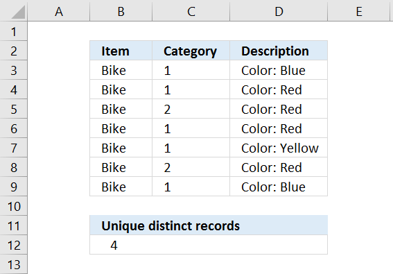
Table of Contents Count unique distinct records Count records with possible blank rows in data set How to count blank […]
Functions in 'Statistical' category
The FREQUENCY function function is one of 73 functions in the 'Statistical' category.
Excel function categories
Excel categories
23 Responses to “How to use the FREQUENCY function”
Leave a Reply
How to comment
How to add a formula to your comment
<code>Insert your formula here.</code>
Convert less than and larger than signs
Use html character entities instead of less than and larger than signs.
< becomes < and > becomes >
How to add VBA code to your comment
[vb 1="vbnet" language=","]
Put your VBA code here.
[/vb]
How to add a picture to your comment:
Upload picture to postimage.org or imgur
Paste image link to your comment.
hi
how to find missing numbers range 1-49 from following line
06 11 17 33 37 47
05 06 12 14 22 34
03 20 35 41 48 49
08 12 17 24 25 45
03 10 18 22 29 45
13 16 22 23 39 43
03 10 17 31 36 45
02 24 32 37 43 49
10 16 27 28 29 42
02 35 38 39 40 48
08 23 34 36 44 47
09 16 21 26 28 29
10 15 32 33 39 41
04 11 20 33 43 45
01 08 21 22 27 36
04 12 25 36 43 49
09 12 23 26 34 43
19 23 24 30 34 46
08 17 20 21 31 45
04 06 17 27 36 48
07 08 19 28 32 41
13 17 26 30 39 47
10 15 20 29 32 43
13 19 22 25 27 45
04 09 19 21 25 42
01 12 24 37 44 47
08 19 31 34 38 42
11 14 31 33 34 47
19 22 32 33 38 48
08 13 14 20 37 40
03 08 10 13 41 47
01 02 14 16 26 30
30 34 36 37 41 49
01 02 14 17 22 37
03 09 28 34 39 47
01 07 09 15 35 37
13 14 19 24 32 33
01 09 10 24 31 41
11 14 19 23 35 41
25 26 27 31 42 49
14 16 21 26 37 48
11 22 24 34 35 40
05 10 12 13 15 17
05 12 18 22 44 45
Narend,
find missing numbers range 1-49 from each row or the whole range?
See this blog post: https://www.get-digital-help.com/identify-missing-numbers-in-a-range-in-excel/
Hello,
I just stumbled over this website and it's fascinating.
Still I hope you can help me with the topic above since I get a #NUM error when using the formula. I want to extrac an unique list of data sorted by their occurance. For me it seems it works only partially.
Hope you can help. Thanks
Irina,
I have pretty much changed everyting in this post. I hope it works now.
Thanks for your comment!
How can you use large with multiple criteria?? Example looking for top 5 of a list based on name, state and city..
Sara,
See this post: https://www.get-digital-help.com/unique-distinct-records-sorted-by-frequency/
Hi Oscar, how do you exclude blanks from this? The formula to create the unique distinct list, sorted by occurrences from large to small is almost exactly what I'm looking for...I just can't seem to figure out where to wrap the IF(ISBLANK() to get this thing to exclude blanks.
Joe,
Array formula in cell D3:
See attached file:
unique-sorted-by-occurances-blanks.xls
Hi Oscar,
brilliant formulas here. Helped me out a lot.
Is it actually possible to sort list elements with an equal number of occurrence in alphabetical order?
Thanks in advance,
Gerald.
Gerald,
Great question!
See this file: unique-sorted-by-occurances-sorted-in-alphabetical-order.xls
Fantastic! Thanks a lot Oscar.
Oscar,
Often I see spreadsheets that have used the Histogram feature (in the Data Analysis Tools) to create a frequency distribution. Although this works, it has one major drawback: it is static. If the data changes, then the Histogram count does not update so it may be wrong.
Using the FREQUENCY function, as you demonstrate in this article, is a much better solution.
Cheers,
Bob.
hi
i saw your all solutions about unique list but not find my answer. my question is ....i have 4 columns emp.no, name, code and program
emp no name code prog
903 a1 p30 find
903 a1 p40 generate report
903 a1 p30 find
904 a2 p40 generate reports
904 a2 p40 error
903 a1 p20 error
903 a1 p30 find
904 a2 p40 generate reports
now i want unique row with coount(means how many times row reapeting)
anju,
read this post:
Filter unique distinct row records in excel 2007
now i want unique row with coount(means how many times row reapeting)
Use the countifs function to count rows:
COUNTIFS function
Hi,
How do I create a new unique distinct list from their income?
Client A -$5
Client A -$5
Client B - $1
Client C - $2
Client A - $2
Results will be:
Client A $12
Client C $2
Client B $1
[…] Frequency function […]
Hmm, seems like it's half Frequency's fault and half Mod's fault.
=MOD(1.3,1) causes the issue, but =MOD(2.3,1) does not. Yet =MOD(1.3,1)=0.3 returns true. Very interesting catch!
The same thing happens if I use INT function to extract the decimal part of a number.
Like this:
=1.1-INT(1.1)
=1.2-INT(1.2)
=1.3-INT(1.3)
=1.4-INT(1.4)
Both Excel 2010 and 2013 yields the same output.
[…] Cronquist is having a problem with the FREQUENCY function, when combined with the MOD function. Can you explain the […]
It's our old friend the floating point error.
https://www.office-loesung.de/p/viewtopic.php?f=166&t=693238#p2874564
MOD(ROW(A13)/10,1)=0,3 is TRUE but
(MOD(ROW(A13)/10,1)-0,3) is 5,55111512312578E-17 but
MOD(ROW(A13)/10,1)-0,3 is 0
So, ROUND(MOD(ROW(11:14)/10,1),1) should work.
XLarium,
Thank you for commenting, I didn't know this.
I found this:
https://support.microsoft.com/en-us/kb/78113
That explains why this happens.
This is a very good formula. At first, it was hard to understand.
With the help of debugger key F9, I was able to analyze it to gain
a better understanding.
Here is my notes using cell D5 as an example.
In cell D5, we have:
=INDEX(List, MATCH(LARGE(IF(COUNTIF($D$2:$D4, List)=0, COUNTIF(List, List),
""), 1), COUNTIF(List, List)*(COUNTIF($D$2:$D4, List)=0), 0))
To make it more readable, we substitute them with array formula:
=INDEX(List,MATCH(LARGE(occurArrayExLargerB,1),occurArrayExLarger0,0))
where
occurArray = COUNTIF(List,List)
occurArrayExLarger0 = (COUNTIF($D$2:$D4,List)=0)*occurArray
occurArrayExLargerB =IF(COUNTIF($D$2:$D4,List)=0, occurArray,"")
To debug, we highlight the individual array formula and press F9 to get their intermediate values:
COUNTIF($D$2:$D4,List) = {0;1;1;0;1;0;1;1;0;1;0;1}
COUNTIF($D$2:$D4,List)=0 (exclusion logic)
{TRUE;FALSE;FALSE;TRUE;FALSE;TRUE;FALSE;FALSE;TRUE;FALSE;TRUE;FALSE}
occurArray = {2;4;4;2;4;2;3;4;2;3;1;3}
occurArrayExLarger0 = {2;0;0;2;0;2;0;0;2;0;1;0}
which means to Exclude Larger occurrences (3 and 4) with 0
occurArrayExLargerB = {2;"";"";2;"";2;"";"";2;"";1;""}
which means to Exclude Larger occurrences (3 and 4) with Blank ""
=INDEX(List, MATCH(2,occurArrayExLarger0,0)))
=INDEX(List, 1) = "DD"
This will result in #NUM! for cell beyond D7 because there are only
5 unique cells. To expand dynamically, we wrap it around with ISERROR:
=IF(ISERROR(
INDEX(List,MATCH(LARGE(occurArrayExLargerB,1),occurArrayExLarger0,0))),"",
INDEX(List,MATCH(LARGE(occurArrayExLargerB,1),occurArrayExLarger0,0)))
Now we can copy and paste it to any cell in column D.
This is the reason we need to define occurArrayExLargerB in addition to
occurArrayExLarger0 because function LARGE(all"",1) will result in #NUM!.
If it wasn't for #NUM! showing in cells beyond D7, we could simplify it to:
=INDEX(List,MATCH(LARGE(occurArrayExLarger0,1),occurArrayExLarger0,0))
without defining a new array formula occurArrayExLargerB.
I tried frequency function many time but it does not work as shown in Example 2.
- First, I type the formula: =Frequency(B3:B10,C:C5)
- Then I press ctrl+shift+enter
- The result is only one value of 3 instead of an array as it is supposed to be
Please tell me why? Thank you