Array Manipulation Functions
Table of Contents
- How to use the CHOOSECOLS function
- How to use the CHOOSEROWS function
- How to use the DROP function
- How to use the EXPAND function
- How to use the HSTACK function
- How to use the TAKE function
- How to use the TOCOL function
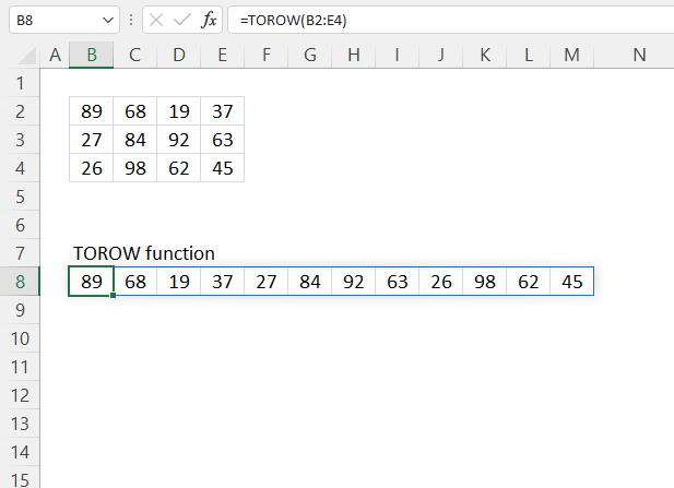
- How to use the TOROW function
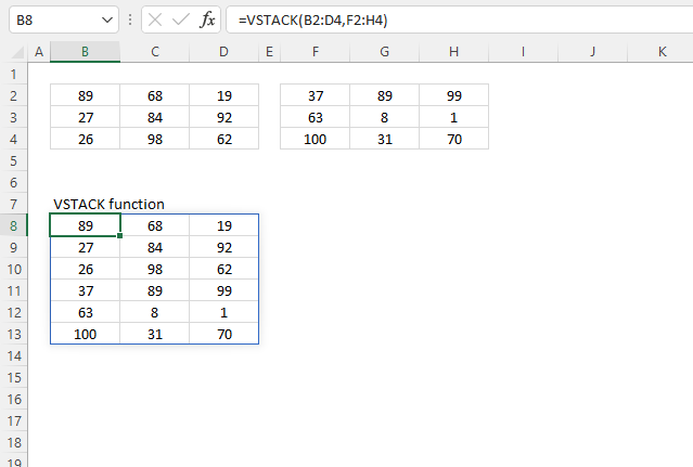
- How to use the VSTACK function
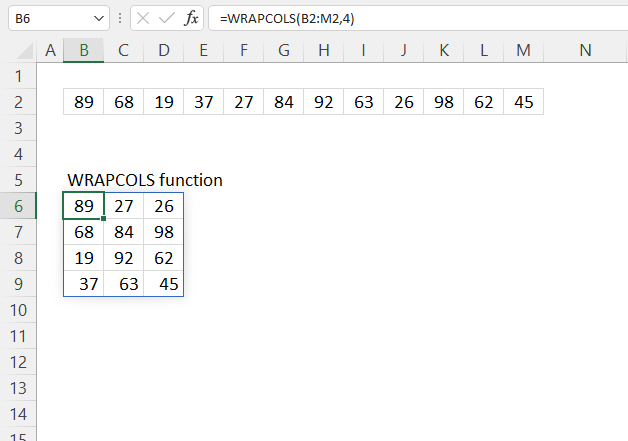
- How to use the WRAPCOLS function
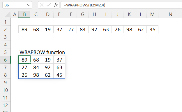
- How to use the WRAPROWS function
1. How to use the CHOOSECOLS function
What is the CHOOSECOLS function?
The CHOOSECOLS function returns given columns from a cell range or array.
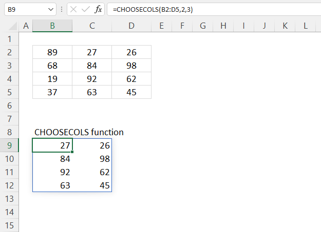
The image above shows a set of values in cell range B2:D5, I have enetered a CHOOSECOLS formula in cell B9:
It spills values to cells below and to the right of cell B9 as far as needed, this is done automatically. This specific formula in cell B9 extracts columns 2 and three from B2:D5.
The CHOOSECOLS function is available to Excel 365 users and is in the "Array manipulation" category.
Table of Contents
- CHOOSECOLS Function Syntax
- CHOOSECOLS Function Arguments
- CHOOSECOLS Function example
- How to combine specific cell range columns - Excel 365
- How to combine specific columns based on a given value - Excel 365
- How to combine columns using negative values - Excel 365
- CHOOSECOLS function returns a #VALUE! error
- Extract values from given columns and return the list in random order - Excel 365
- Join multiple non-adjacent cell ranges and return given columns (3D range) - Excel 365
- Get Excel file
1.1. CHOOSECOLS Function Syntax
CHOOSECOLS(array, col_num1, [col_num2], …)
1.2. CHOOSECOLS Function Arguments
array | Required. The source cell range or array. |
col_num1 | Required. A number represents the column in a given cell range. |
[col_num2] | Optional. Extra column numbers to be extracted. |
1.3. CHOOSECOLS Function example
The picture above shows how the CHOOSECOLS function extracts the second and third column from cell range B2:D5.
Dynamic array formula in cell B9:
The image contains numbers below each column in cell range B2:D5, the numbers lets you easily identify columns 2 and 3. The output is shown in cell B9, columns 2 and 3 are extracted from B2:D5.
Excel 365 dynamic array formulas are different than regular array formulas. The former are entered as regular formulas, however they automatically spill values below and to the right as far as needed. A #SPILL! error is displayed if a cell is not empty where spilling needs to be returned. Simply delete the value and the formula works again.
1.3.1 Explaining formula
Step 1 - CHOOSECOLS function
The CHOOSECOLS function has two required arguments and one optional. The optional argument is not limited to one value, it can be up to at least 254 arguments.
CHOOSECOLS(array, col_num1, [col_num2], …)
Step 2 - Populate arguments
array - B2:D5
col_num1 - 2
[col_num2] - 3
Step 3 - Evaluate function
CHOOSECOLS(B2:D5, 2, 3)
becomes
CHOOSECOLS({89, 27, 26;
68, 84, 98;
19, 92, 62;
37, 63, 45}, 2, 3)
and returns
{27, 26; 84, 98;
92, 62; 63, 45}
The image below shows the array in cell range B9:C12.
1.4. How to combine specific cell range columns - CHOOSECOLS Function
The CHOOSECOLS function lets you use an array in the arguments, the image above demonstrates a CHOOSECOLS function that uses an array in the second argument. This means that you are not limited to arguments, you can use an array in one argument. This makes it possible to use a lot more than 254 columns.
Dynamic array formula in cell B9:
The image above has values in cell range B2:D5, I have entered blue numbers below each column so you can more easily see the extracted columns. Columns 1 and 3 are returned to a dynamic array that spills values to cells below and to the right as far as needed.
This makes the CHOOSECOLUMNS function useful for combining specific columns from a given data set., this in return makes it even easier to work with arrays in Excel 365 than in earlier Excel versions.
Explaining formula
Step 1 - Populate the array
The curly brackets let you build an array that you can use in most but not all Excel functions. The ; semicolon is a delimiting character that separates values row by row.
The CHOOSE function requires numbers separated with semicolons or whatever row delimiting character you use.
{1; 3}
Step 2 - CHOOSECOLS function
CHOOSECOLS(array, col_num1, [col_num2], …)
CHOOSECOLS(B2:D5, {1; 3})
becomes
CHOOSECOLS({89, 27, 26;
68, 84, 98;
19, 92, 62;
37, 63, 45}, {1; 3})
and returns
{89, 26;
68, 98;
19, 62;
37,45}
1.5. How to combine specific columns based on a given value - CHOOSECOLS Function
The section shows how to return specific columns based on a string containing numbers delimited by a character. The TEXTSPLIT function separates values into an array.
Cell F2 contains the foloowing thext string: 1,2 This string is separated into an array using the comma as a delimiting character. The array is then used to extract columns 1 and 2 from cell range B2:D5.
Dynamic array formula in cell B9:
This is handy if the Excel user needs to specify the given columns in a cell, which in turn makes it more user friendly than editing hard-coded values in a formula. Working with arrays has never been easier, the new Excel 365 functions are very much so appreciated.
Explaining formula
Step 1 - Split text
The TEXTSPLIT function lets you split a string into an array across columns and rows based on delimiting characters.
TEXTSPLIT(Input_Text, col_delimiter, [row_delimiter], [Ignore_Empty])
TEXTSPLIT(F2,,",")
becomes
TEXTSPLIT("1,2", , ",")
and returns {"1"; "2"}.
Note the double quotes, Excel handles these values as text values. The next step converts text values to numbers.
Step 2 - Convert text to numbers
The asterisk lets you multiply numbers in an Excel formula, I am using it here to convert text to numbers.
TEXTSPLIT(F2,,",")*1
becomes
{"1"; "2"}*1
and returns {1; 2}.
Step 3 - CHOOSECOLS function
CHOOSECOLS(B2:D5,TEXTSPLIT(F2,,",")*1)
becomes
CHOOSECOLS(B2:D5, {1; 2})
becomes
CHOOSECOLS({89, 27, 26;
68, 84, 98;
19, 92, 62;
37, 63, 45}, {1; 2})
and returns
{89, 27;
68, 84;
19, 92;
37, 63}
The image below shows the array described above in cell B9, the dynamic array formula spills values cells below and to the right as far as needed.
1.6. How to combine columns using negative values - CHOOSECOLS Function
The CHOOSECOLS function lets you also use negative numbers, this will make the function count columns from right to left.
This is useful if you have a large array containing many columns. If you need to extract columns located to the far right, instead of counting columns from left to right you can use negative integers and count from right to left. This may save you time and less prone to errors.
Formula in cell B9:
CHOOSECOLS(array, col_num1, [col_num2], …)
The image above shows an array in cell range B2:C5. The formula in cell B9 extracts the last column and the next one counting from right to left using negative numbers.
1.7. CHOOSECOLS function returns a #VALUE! error
The CHOOSECOLS function returns a #VALUE! error when no values can be displayed.Here is a scenario when this can happen.
The image above displays an array in cell range B2:D5, the formula in cell B9 tries to extract the fifth column from B2:D5, however, there are only three columns in cell range B2:D5.
This makes it impossible for the CHOOSECOLS function to extract the fifth column thus returning the #VALUE error. You can catch errors using the IFERROR function, however, hiding errors is not always great. The downside is that if hide errors you make them much harder to find. Finding errors is most important in order to troubleshoot and find a solution to the problem.
1.8. Extract values from given columns and return the list in random order - CHOOSECOLS function
The image above shows an array in cell range B2:D5. The formula in cell B8 returns values in random order from columns two and three in B2:D5.
Dynamic array formula in cell B8:
The result in cell B8 shows an array with the same size as column 2 and 3 from cell range B2;D5. However, the values from column 2 and 3 are in random order. Note that the formula also only returns values from column 2 and 3 but in random order.
1.8.1 Explaining formula in cell B8
Step 1 - Filter columns 2 and 3
CHOOSECOLS(B2:D5, 2, 3)
becomes
CHOOSECOLS({89, 27, 26;
68, 84, 98;
19, 92, 62;
37, 63, 45}, 2, 3)
and returns
{27,26;
84,98;
92,62;
63,45}
Step 2 - Rearrange values to a single row
The TOROW function rearranges values from a 2D cell range or array to a single row.
TOROW(array, [ignore], [scan_by_col])
TOROW(CHOOSECOLS(B2:D5,2,3))
becomes
TOROW({27,26;
84,98;
92,62;
63,45}
and returns
{27, 26, 84, 98, 92, 62, 63, 45}.
Step 3 - Count cells
The COLUMNS function returns the number of columns in a given cell range or array.
COLUMNS(array)
COLUMNS(TOROW(CHOOSECOLS(B2:D5,2, 3)))
becomes
COLUMNS({27, 26, 84, 98, 92, 62, 63, 45})
and returns 8.
Step 4 - Count rows
The ROWS function returns the number of rows in a given cell range or array.
ROWS (array)
ROWS(CHOOSECOLS(B2:D5,2, 3))
becomes
ROWS({27,26;
84,98;
92,62;
63,45})
and returns 4.
Step 5 - Create random decimal numbers
The RANDARRAY function returns a table of random numbers across rows and columns.
RANDARRAY([rows], [columns], [min], [max], [whole_number])
RANDARRAY(,COLUMNS(TOROW(CHOOSECOLS(B2:D5,2, 3))))
becomes
RANDARRAY(,6)
and returns
{0.215398134613085, 0.390607168196479, ... ,0.83231474462401}.
Step 6 - Rearrange values in random order
The SORTBY function allows you to sort values from a cell range or array based on a corresponding cell range or array.
SORTBY(array, by_array1, [sort_order1], [by_array2, sort_order2],…)
SORTBY(TOROW(CHOOSECOLS(B2:D5,2, 4)),RANDARRAY(,COLUMNS(CHOOSECOLS(B2:D5,2, 3))))
becomes
SORTBY({27,26;
84,98;
92,62;
63,45}, {0.215398134613085, 0.390607168196479, ... ,0.83231474462401})
and returns
{84, 98, 27, 92, 62, 26, 45, 63}
Step 7 - Rearrange values to the original array size
The WRAPCOLS function rearranges values from a single row to a 2D cell range based on a given number of values per column.
WRAPCOLS(vector, wrap_count, [pad_with])
WRAPCOLS(SORTBY(TOROW(CHOOSECOLS(B2:D5,2, 4)),RANDARRAY(,COLUMNS(TOROW(CHOOSECOLS(B2:D5,2, 4))))),ROWS(CHOOSECOLS(B2:D5,2, 3)))
becomes
WRAPCOLS({63, 37, 45, 98, 84, 68}, ROWS(CHOOSECOLS(B2:D5,2, 3)))
becomes
WRAPCOLS({84, 98, 27, 92, 62, 26, 45, 63}, 4)
and returns
{84, 98; 27, 92; 62, 26; 45, 63}.
Step 8 - Shorten formula
The LET function lets you name intermediate calculation results which can shorten formulas considerably and improve performance.
LET(name1, name_value1, calculation_or_name2, [name_value2, calculation_or_name3...])
WRAPCOLS(SORTBY(TOROW(CHOOSECOLS(B2:D5, 2, 3)), RANDARRAY(, COLUMNS(TOROW(CHOOSECOLS(B2:D5, 2, 3))))), TOROW(CHOOSECOLS(B2:D5, 2, 3)))
becomes
LET(z, CHOOSECOLS(B2:D5, 2, 3), x, TOROW(z), WRAPCOLS(SORTBY(x, RANDARRAY(, COLUMNS(x))), ROWS(z)))
1.9. Join multiple non-adjacent cell ranges and return given columns (3D range) - CHOOSECOLS function
The image above shows three data sets in cell ranges B3:D6, F3:H6, and J3:L6. The formula in cell B9 merges these three non-contiguous cell ranges vertically and returns columns 1 and 2.
Dynamic array formula in cell B9:
This is a rather complicated manipultaion of three different cell ranges. The CHOOSECOLS and VSTACK functions makes it super easy to join the cell ranges and then extract only column 1 and 2.
This formula can be really useful if you want to work with cell ranges across multiple worksheets and apply different calculations, for example, like finding the average or return unique distinct values. These types of calculations have never been easier with the new Array manipulation functions.
1.9.1 Explaining formula
Step 1 - Stack values horizontally
The VSTACK function lets you combine cell ranges or arrays, it joins data to the first blank cell at the bottom of a cell range or array (vertical stacking)
VSTACK(array1, [array2],...)
VSTACK(B3:D6, F3:H6, J3:L6)
becomes
VSTACK({"Peach", 43, 1.03;"Blueberry", 39, 1.48;"Apple", 46, 1.1;"Grapefruit", 14, 0.72}, {"Mandarin", 29, 0.78;"Raspberry", 33, 1.07;"Plum", 25, 0.9;"Mango", 37, 1.13}, {"Pear", 17, 0.63;"Orange", 31, 1.06;"Lime", 17, 1.27;"Kiwi", 45, 0.58})
and returns
{"Peach", 43, 1.03;
"Blueberry", 39, 1.48;
"Apple", 46, 1.1;
"Grapefruit", 14, 0.72;
"Mandarin", 29, 0.78;
"Raspberry", 33, 1.07;
"Plum", 25, 0.9;
"Mango", 37, 1.13;
"Pear", 17, 0.63;
"Orange", 31, 1.06;
"Lime", 17, 1.27;
"Kiwi", 45, 0.58}
Step 2 - Filter given rows
CHOOSECOLS(VSTACK(B3:D6, F3:H6, J3:L6),1, 2)
becomes
CHOOSECOLS({"Peach", 43, 1.03;
"Blueberry", 39, 1.48;
"Apple", 46, 1.1;
"Grapefruit", 14, 0.72;
"Mandarin", 29, 0.78;
"Raspberry", 33, 1.07;
"Plum", 25, 0.9;
"Mango", 37, 1.13;
"Pear", 17, 0.63;
"Orange", 31, 1.06;
"Lime", 17, 1.27;
"Kiwi", 45, 0.58}, 1, 5, 9)
and returns
{"Peach", 43;
"Blueberry", 39;
"Apple", 46;
"Grapefruit", 14;
"Mandarin", 29;
"Raspberry", 33;
"Plum", 25;
"Mango", 37;
"Pear", 17;
"Orange", 31;
"Lime", 17;
"Kiwi", 45}
How to use the CHOOSECOLS functionv2
Useful links
CHOOSECOLS function - Microsoft support
CHOOSECOLS Function in Excel: Explained
CHOOSECOLS function in Excel to get columns from array or range
2. How to use the CHOOSEROWS function
What is the CHOOSEROWS function?
The CHOOSEROWS function returns given rows from a cell range or array.
The CHOOSEROWS function is available to Excel 365 users and is in the "Array manipulation" category.
Table of Contents
- CHOOSEROWS Function Syntax
- CHOOSEROWS Function Arguments
- CHOOSEROWS Function example
- CHOOSEROWS Function example - array
- CHOOSEROWS Function example - split text to array
- CHOOSEROWS Function example - negative values
- CHOOSEROWS Function errors
- CHOOSEROWS Function - values in random order
- CHOOSEROWS Function - multiple source ranges
- Get every other row
- Get Excel file
2.1. CHOOSEROWS Function Syntax
CHOOSEROWS(array, row_num1, [row_num2], …)
2.2. CHOOSEROWS Function Arguments
array | Required. The source cell range or array. |
row_num1 | Required. A number representing the row in a given cell range. |
[row_num2] | Optional. Extra row numbers to be extracted. |
2.3. CHOOSEROWS Function example
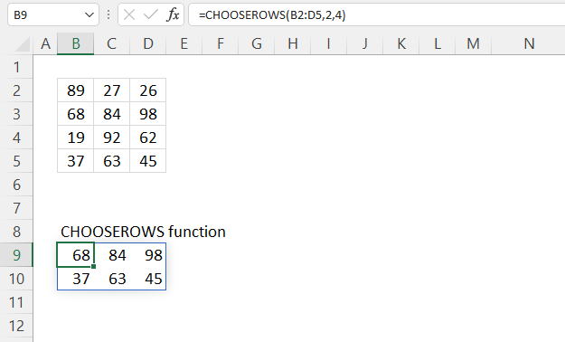
The picture above shows how the CHOOSEROWS function extracts the second and fourth row from cell range B2:D5 leaving the first and third row out.
Dynamic array formula in cell B9:
The image above shows values in cell range B2:D5, the formula in cell B9 extracts rows 2 and 4 and merges these rows to a single array. The array has the same number of columns as B2:D5 except that it now only contains two rows.
Excel 365 dynamic array formulas are different than regular array formulas in earlier Excel versions. Excel 365 dynamic array formulas are entered as regular formulas, however they automatically spill values below and to the right as far as needed.
If the destination range is not empty a #SPILL! error is shown. It is easy to fix this problem, delete the value and the Excel 365 formula works again.
2.3.1 Explaining formula
Step 1 - CHOOSEROWS function
CHOOSEROWS(array, row_num1, [row_num2], …)
Step 2 - Populate arguments
array - B2:D5
row_num1 - 2
[row_num2] - 4
Step 3 - Evaluate function
CHOOSEROWS(B2:D5, 2, 4)
becomes
CHOOSEROWS({89, 27, 26;
68, 84, 98;
19, 92, 62;
37, 63, 45}, 2)
and returns
{68, 84, 98;
37, 63, 45}
The returned array is shown in B9:E10 in the image below.
2.4. CHOOSEROWS Function example - array
The CHOOSEROWS function lets you use an array in the arguments, the image above shows an array in the second argument {1;4}. An array begins with a curly bracket { and ends with a curly bracket }. These characters tell Excel that this is an array.
Using an array in an argument lets you specify the rows which you want to keep, the remaining rows are filtered out. This lets you enter rows in one argument only if you prefer.
Values in an array are delimited by one character for rows and one for columns, which you use are determined by your regional settings in windows. My settings use a semicolon for rows and a comma for columns.
Dynamic array formula in cell B9:
This example demonstrates values in cell range B2:D5, displayed in the image above. The formula in cell B9 returns an array containing rows 1 and 4, the number of columns match the original array B2:D5. Use the CHOOSECOLS function when you want to resize an array based on rows, for example, if you want to calculate the median or frequency based on a particular row or rows in an array.
This was very difficult in earlier versions, Excel 365 is a big step forward. Excel 365 spills values to cell B9 and cells below and to the right as far as needed. A #SPILL error is shown if a cell contains a value. Delete the value so the formula can show all values in the array.
Explaining formula
Step 1 - Populate the array
The curly brackets let you build an array that you can use in most but not all Excel functions. The ; semicolon is a delimiting character that separates values row by row.
The CHOOSE function requires numbers separated with semicolons or whatever row delimiting character you use.
{1; 4}
Step 2 - CHOOSEROWS function
CHOOSEROWS(array, row_num1, [row_num2], …)
CHOOSEROWS(B2:D5, {1; 4})
becomes
CHOOSEROWS({89, 27, 26;
68, 84, 98;
19, 92, 62;
37, 63, 45}, {1; 4})
and returns
{89, 27, 26;
37, 63, 45}
2.5. CHOOSEROWS Function example - split text to array
The section shows how to return specific rows based on a string containing numbers. Cell F2 contains a text value containing numbers delimited by a comma.
The TEXTSPLIT function separates the values in to an array that the CHOOSEROWS function can use to filter the given rows.
Dynamic array formula in cell B9:
The image above shows values in cell range B2:D5, the specified rows is in cell F2. The formula in cell B9 returns rows 1, 3 and 4 to cell B9 based on the specified numbers in cell F2. Excel 365 spills values to cell B9 and cells below and to the right as far as needed.
A #SPILL error is returned if a cell is not empty, this restricts the dynamic array formula to show all values in the array. Simply delete the cell containing the value and the formula works again.
Explaining formula
Step 1 - Split text
The TEXTSPLIT function lets you split a string into an array across columns and rows based on delimiting characters.
TEXTSPLIT(Input_Text, col_delimiter, [row_delimiter], [Ignore_Empty])
TEXTSPLIT(F2,,",")
becomes
TEXTSPLIT("1,3,4",,",")
and returns {"1"; "3"; "4"}. Note the double quotes, Excel handles these values as text values. The next step converts text values to numbers.
Step 2 - Convert text to numbers
The asterisk lets you multiply numbers in an Excel formula, I am using it here to convert text to numbers.
TEXTSPLIT(F2,,",")*1
becomes
{"1"; "3"; "4"}*1
and returns {1; 3; 4}.
Step 3 - CHOOSEROWS function
CHOOSEROWS(B2:D5,TEXTSPLIT(F2,,",")*1)
becomes
CHOOSEROWS(B2:D5, {1; 3; 4})
becomes
CHOOSEROWS({89, 27, 26;
68, 84, 98;
19, 92, 62;
37, 63, 45}, {1; 3; 4})
and returns
{89,27,26;
19,92,62;
37,63,45}
2.6. CHOOSEROWS Function example - negative values
The CHOOSEROWS function lets you use negative numbers, this will make the function count from the bottom or from the end. This is really helpful if you array is large and you want to select rows close to the end of the array.
This example uses value -4 to extract the fourth row counting from the bottom. In this example the array consists of only four rows. This means that the extracted row is the first row in cell range B2:D5.
Formula in cell B9:
Use negative row numbers if it is easier to count from the end instead of the beginning. The image above shows the values to the right of B2:D5, they are blue and 1 is the last row. The next row counted from the bottom is two etc.
CHOOSEROWS(array, row_num1, [row_num2], …)
2.7. CHOOSEROWS function error
The CHOOSEROWS function returns a #VALUE! error when no values can be displayed.Here is a scenario when this can happen.
The image above displays an array in cell range B2:D5, the formula in cell B9 tries to extract the fifth row from B2:D5, however, there are only four rows in cell range B2:D5.
This makes it impossible for the CHOOSECOLS function to extract the fifth row thus returning the #VALUE error. You can catch errors using the IFERROR function, however, hiding errors is not always great. The downside is that if hide errors you make them much harder to find. Finding errors is most important in order to troubleshoot and find a solution to the problem.
2.8. CHOOSEROWS function - values in random order
The image above shows a formula that returns values in random order from rows 2 and 4 in a 2D cell range. 2D meaning a two dimensional cell range or a cell range containing both rows and columns. The source data range is in B2:D5, it contains numbers in no particular order.
Dynamic array formula in cell B8:
The formula in cell B8 extracts rows 2 and 4 and returns the corresponding values in random order. The formula spills values below cell B8 and to the right as far as needed.
This formula is useful if you want to extract specific values from an array based on given rows and return the values in random order.
2.8.1 Explaining formula in cell B8
Step 1 - Remove two first rows
CHOOSEROWS(B2:D5, 2, 4)
becomes
CHOOSEROWS({89, 27, 26;
68, 84, 98;
19, 92, 62;
37, 63, 45}, 2, 4)
and returns
{68,84,98;
37,63,45}.
Step 2 - Rearrange values to a single row
The TOROW function rearranges values from a 2D cell range or array to a single row.
TOROW(array, [ignore], [scan_by_col])
TOROW(CHOOSEROWS(B2:D5,2,4))
becomes
TOROW({68,84,98;
37,63,45})
and returns
{68, 84, 98; 37, 63, 45}.
Step 3 - Count cells
The COLUMNS function returns the number of columns in a given cell range or array.
COLUMNS(array)
COLUMNS(TOROW(CHOOSEROWS(B2:D5,2, 4)))
becomes
COLUMNS({68, 84, 98, 37, 63, 45})
and returns 6.
Step 4 - Count rows
The ROWS function returns the number of rows in a given cell range or array.
ROWS (array)
ROWS(CHOOSEROWS(B2:D5,2, 4))
becomes
ROWS({68, 84, 98; 37, 63, 45})
and returns 2.
Step 5 - Create random decimal numbers
The RANDARRAY function returns a table of random numbers across rows and columns.
RANDARRAY([rows], [columns], [min], [max], [whole_number])
RANDARRAY(,COLUMNS(TOROW(CHOOSEROWS(B2:D5,2, 4))))
becomes
RANDARRAY(,6)
and returns
{0.215398134613085, 0.390607168196479, ... ,0.83231474462401}.
Step 6 - Rearrange values in random order
The SORTBY function allows you to sort values from a cell range or array based on a corresponding cell range or array.
SORTBY(array, by_array1, [sort_order1], [by_array2, sort_order2],…)
SORTBY(TOROW(CHOOSEROWS(B2:D5,2, 4)),RANDARRAY(,COLUMNS(CHOOSEROWS(B2:D5,2, 4))))
becomes
SORTBY({68, 84, 98, 37, 63, 45}, {0.215398134613085, 0.390607168196479, ... ,0.83231474462401})
and returns
{63, 37, 45, 98, 84, 68}
Step 7 - Rearrange values to the original array size
The WRAPCOLS function rearranges values from a single row to a 2D cell range based on a given number of values per column.
WRAPCOLS(vector, wrap_count, [pad_with])
WRAPCOLS(SORTBY(TOROW(CHOOSEROWS(B2:D5,2, 4)),RANDARRAY(,COLUMNS(TOROW(CHOOSEROWS(B2:D5,2, 4))))),ROWS(CHOOSEROWS(B2:D5,2, 4)))
becomes
WRAPCOLS({63, 37, 45, 98, 84, 68}, ROWS(CHOOSEROWS(B2:D5,2, 4)))
becomes
WRAPCOLS({63, 37, 45, 98, 84, 68}, 2)
and returns
{63, 37, 45; 98, 84, 68}.
Step 8 - Shorten formula
The LET function lets you name intermediate calculation results which can shorten formulas considerably and improve performance.
LET(name1, name_value1, calculation_or_name2, [name_value2, calculation_or_name3...])
WRAPCOLS(SORTBY(TOROW(CHOOSEROWS(B2:D5, 2, 4)), RANDARRAY(, COLUMNS(TOROW(CHOOSEROWS(B2:D5, 2, 4))))), TOROW(CHOOSEROWS(B2:D5, 2, 4)))
becomes
LET(z, CHOOSEROWS(B2:D5, 2, 4), x, TOROW(z), WRAPCOLS(SORTBY(x, RANDARRAY(, COLUMNS(x))), ROWS(z)))
2.9. CHOOSEROWS Function - multiple source ranges
The picture above shows a formula that merges three non-contiguous cell ranges and shows rows 1, 5, and 9. It shows three data sets in cell ranges B3:D6, F3:H6, and J3:L6. The formula in cell B9 merges these three non-contiguous cell ranges vertically and returns rows 1, 5, and 9.
Dynamic array formula in cell B9:
This is a rather complicated manipulation of three different cell ranges. The CHOOSEROWS and VSTACK functions makes it super easy to join the cell ranges and then extract only rows 1, 5, and 9.
This formula can be really useful if you want to work with cell ranges across multiple worksheets and apply different calculations, for example, like finding the average or return unique distinct values. These types of calculations have never been easier with the new Array manipulation functions.
2.9.1 Explaining formula
Step 1 - Stack values horizontally
The VSTACK function lets you combine cell ranges or arrays, it joins data to the first blank cell at the bottom of a cell range or array (vertical stacking)
VSTACK(array1, [array2],...)
VSTACK(B3:D6, F3:H6, J3:L6)
becomes
VSTACK({"Peach", 43, 1.03;"Blueberry", 39, 1.48;"Apple", 46, 1.1;"Grapefruit", 14, 0.72}, {"Mandarin", 29, 0.78;"Raspberry", 33, 1.07;"Plum", 25, 0.9;"Mango", 37, 1.13}, {"Pear", 17, 0.63;"Orange", 31, 1.06;"Lime", 17, 1.27;"Kiwi", 45, 0.58})
and returns
{"Peach", 43, 1.03;
"Blueberry", 39, 1.48;
"Apple", 46, 1.1;
"Grapefruit", 14, 0.72;
"Mandarin", 29, 0.78;
"Raspberry", 33, 1.07;
"Plum", 25, 0.9;
"Mango", 37, 1.13;
"Pear", 17, 0.63;
"Orange", 31, 1.06;
"Lime", 17, 1.27;
"Kiwi", 45, 0.58}
Step 2 - Filter given rows
CHOOSEROWS(VSTACK(B3:D6, F3:H6, J3:L6),1, 5, 9)
becomes
CHOOSEROWS({"Peach", 43, 1.03;
"Blueberry", 39, 1.48;
"Apple", 46, 1.1;
"Grapefruit", 14, 0.72;
"Mandarin", 29, 0.78;
"Raspberry", 33, 1.07;
"Plum", 25, 0.9;
"Mango", 37, 1.13;
"Pear", 17, 0.63;
"Orange", 31, 1.06;
"Lime", 17, 1.27;
"Kiwi", 45, 0.58}, 1, 5, 9)
and returns
{"Peach", 43, 1.03;
"Mandarin", 29, 0.78;
"Pear", 17, 0.63}
2.10. CHOOSEROWS Function - get every other row
The formula in cell F4 extracts every other row in cell range B3:D14, the dynamic array formula calculates how many rows are needed automatically based on the number of rows in the given cell reference.
Formula in cell F4:
The source cell range is B3:D14 and every other row is highlighted, in other words the cell background color is different.This is done so you can easily see that the formula extracts every other row beginning with row number 1.
The formula extracts rows 1 to 6 entirely based on the total number of rows in B3:D14. This means that if you change the cell reference B3:D14 to for example B3:D20 every other row is instantly calculated and the corresponding values are returned. There is no need to calculate the row numbers manually, the formula does this for you.
Cell F4 contains the formula and the output contains every other row from cell range B3:D14 as you can see if you compare the output to the source data range. The formula returns a #SPILL error if the destination cells are not empty. Make sure the cells are completely empty and the formula instantly works again.
2.10.1 Explaining formula
Step 1 - Count rows
The ROWS function returns a number corresponding to the number of rows in a given cell reference.
ROWS(array)
ROWS(B3:D14)
returns 12. There are twelve rows in cell reference B3:D14.
Step 2 - Round number up
The ROUNDUP function rounds a number up.
ROUNDUP(number, num_digits)
ROUNDUP(ROWS(B3:D14)/2,0)
becomes
ROUNDUP(12/2,0)
becomes
ROUNDUP(6,0)
and returns 6.
Step 3 - Create a sequence of numbers from 1 to n step 2
The SEQUENCE function creates a list of sequential numbers.
SEQUENCE(rows, [columns], [start], [step])
SEQUENCE(ROUNDUP(ROWS(B3:D14)/2,0), , 1, 2)
becomes
SEQUENCE(6, , 1, 2)
and returns {1; 3; 5; 7; 9; 11}.
Step 4 - Get rows
CHOOSEROWS(B3:D14, SEQUENCE(ROUNDUP(ROWS(B3:D14)/2,0), , 1, 2))
becomes
CHOOSEROWS(B3:D14, {1; 3; 5; 7; 9; 11})
and returns
{"Peach", 43, 1.03;
"Apple", 46, 1.1;
"Mandarin", 29, 0.78;
"Plum", 25, 0.9;
"Pear", 17, 0.63;
"Lime", 17, 1.27}
Useful links
CHOOSEROWS function - Microsoft support
CHOOSEROWS function in Excel to extract rows from array
Excel CHOOSEROWS Function - my online training hub
3. How to use the DROP function
What is the DROP function?
The DROP function removes a given number of rows or columns from a 2D cell range or array.
Use the drop function if know which columns or rows you want to remove, it removes all the rows or columns up to the specified number starting from 1 to n where n is the given number. The DROP function is available to Excel 365 users and is in the "Array manipulation" category.
Table of Contents
- DROP Function Syntax
- DROP Function Arguments
- DROP Function example
- DROP Function example - exclude columns
- DROP Function example - exclude columns and rows
- DROP Function example - negative values
- DROP Function errors
- DROP Function - values in random order
- DROP Function - multiple source ranges
- Get Excel *.xlsx file
3.1. DROP Function Syntax
DROP(array, rows, [columns])
3.2. DROP Function Arguments
array | Required. The source cell range or array. |
rows | Required. The number of contiguous rows to remove, a negative number removes contiguous rows from the end. |
[columns] | Optional. The number of contiguous columns to remove, a negative number removes contiguous rows from the end. |
3.3. DROP Function example
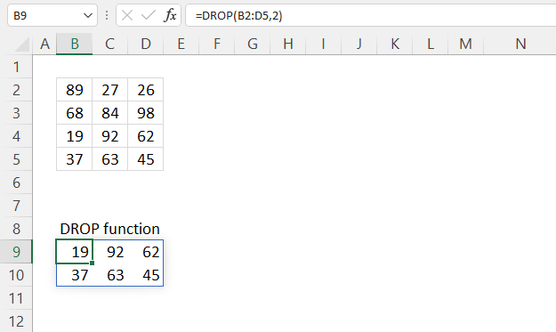
The picture above shows how the DROP function removes the first two rows from cell range B2:D5. For example, number 2 removes both the first row and the second row from the source data range. The DROP function is really useful in combination with the LAMBDA functions SCAN, MAP, REDUCE, BYROW , and BYCOL functions.
Dynamic array formula in cell B9:
B2:D5 contains 4 rows, the output in cell B9 contains only the last two rows in cell B2:D5. This is because the DROP function removes rows from the top and columns from the left. There is an exception to this demonstrated in section 6 below. Hint! Negative values.
The DROP function returns a dynamic array formula meaning that it returns more than one value if needed, however, entering a dynamic array formula is easy. No difference to entering a regular formula, simply press Enter when you are done.
The DROP function returns a #SPILL! error if a cell is not empty in the destination range, in other words, if a cell below C9 has a value then the formula can't show all the values in the array. This results in a #SPILL! error.
To fix this problem you need to delete cells containing values so the formula works as intended.
3.3.1 Explaining formula
Step 1 - DROP function
the DROP function has three arguments, the first and second argument are required and the third argument is optional.
DROP(array, rows, [columns])
Step 2 - Populate arguments
Cell range B2:D5 is used as the array argument, 2 is the rows argument and I leave the columns argument empty.
array - B2:D5
rows - 2
[columns] -
Step 3 - Evaluate function
The following lines show what happens in detail when the DROP function is evaluated in Excel.
DROP(B2:D5, 2)
becomes
DROP({89, 27, 26;
68, 84, 98;
19, 92, 62;
37, 63, 45}, 2)
and returns
{19, 92, 62;
37, 63, 45}
3.4. DROP Function example - remove columns
The image above demonstrates how to remove columns using the DROP function. The image above shows cell range B2:D5 populated with values. The DROP function removes the two first columns from cell range B2:D5 and returns the third column to cell B6 and cells below as far as needed.
Formula in cell B6:
The DROP function has three arguments, the third one is columns and it is optional. The second argument is rows and is also optional if you specify the third argument. This example demonstrates this, the second argument is not specified so the function removes no rows only columns.
3.5. DROP Function example - remove both rows and columns
The image above demonstrates how to remove both rows and columns using the DROP function. Cell range B2:D5 contains values, I have numbered the rows red and they are located to the right of the cell range. The rows argument contains two meaning both the first row and second row is removed from the final array.
The columns are numbered 1 and 2 counting from left to right, they are red. The columns argument contains 2 as well, this means that the first and second column are removed. I have drawn red boxes around the first and second column and the first and second row. The numbers left are in the blue box, they are displayed in cell B9 and cells below.
Formula in cell B9:
DROP(array, rows, [columns])
The DROP function is really useful for removing specific rows and columns in a given array, this was really hard in previous Excel versions and required lots of functions if even possible.
3.6. DROP Function example - negative values
The DROP function lets you use negative arguments, this means that the function removes rows/columns from the end. Cell range B2:D5 contains values, the drop function has three arguments, the second argument is row and is -2 in this example. The third argument is columns and is also -2.
Formula in cell B9:
DROP(array, rows, [columns])
Negative value in the row argument makes the function count from the bottom up, this means that -2 removes the last row and the second last row.
This is also true for the columns argument, -2 removes the last column and the second last column. This leaves us with the first value and the second value, they are in a blue rectangle displayed in the image above. These values are returned from the DROP function in cell B9. This is useful if you need to remove the last column or row or both, no need to count or calculate the number of rows and columns in order to remove the correct ones.
3.7. DROP function error
The DROP function returns a #VALUE! error when no values are displayed. This example, demonstrated in the image above, shows a DROP function using arguments that match or exceed the number of rows and columns in the source data range B2:D5.
Since all values are removed from the source cell range B2:D5 the DROP function returns a #VALUE! error simply because there are no values to display.
3.8. DROP function - values in random order
The image above shows a formula that returns values in random order from the two first rows in a 2D cell range. Cell range B2:D5 contains values, the formula removes the two first rows in B2:D5 and returns the remaining values in random order.
The resulting array has the same size as the source cell range excluding the two first rows. The formula changes the order randomly every time you press function key F9.
Dynamic array formula in cell B8:
This formula is useful if you want to randomize the order for a specific number of rows or columns and not the entire source array.
3.8.1 Explaining formula in cell B8
Step 1 - Remove two first rows
DROP(B2:D5, 2)
becomes
DROP({89, 27, 26;
68, 84, 98;
19, 92, 62;
37, 63, 45}, 2)
and returns
{19, 92, 62;
37, 63, 45}.
Step 2 - Rearrange values to a single row
The TOROW function rearranges values from a 2D cell range or array to a single row.
TOROW(array, [ignore], [scan_by_col])
TOROW(DROP(B2:D5,2))
becomes
TOROW({19, 92, 62;37, 63, 45})
and returns
{19, 92, 62, 37, 63, 45}.
Step 3 - Count cells
The COLUMNS function returns the number of columns in a given cell range or array.
COLUMNS(array)
COLUMNS(TOROW(DROP(B2:D5,2)))
becomes
COLUMNS({19, 92, 62, 37, 63, 45})
and returns 6.
Step 4 - Count rows
The ROWS function returns the number of rows in a given cell range or array.
ROWS (array)
ROWS(DROP(B2:D5,2))
becomes
ROWS({19, 92, 62;37, 63, 45})
and returns 2.
Step 5 - Create random decimal numbers
The RANDARRAY function returns a table of random numbers across rows and columns.
RANDARRAY([rows], [columns], [min], [max], [whole_number])
RANDARRAY(,COLUMNS(TOROW(DROP(B2:D5,2))))
becomes
RANDARRAY(,6)
and returns
{0.215398134613085, 0.390607168196479, ... ,0.83231474462401}.
Step 6 - Rearrange values in random order
The SORTBY function allows you to sort values from a cell range or array based on a corresponding cell range or array.
SORTBY(array, by_array1, [sort_order1], [by_array2, sort_order2],…)
SORTBY(TOROW(DROP(B2:D5,2)),RANDARRAY(,COLUMNS(DROP(B2:D5,2))))
becomes
SORTBY({19, 92, 62, 37, 63, 45}, {0.215398134613085, 0.390607168196479, ... ,0.83231474462401})
and returns
{19, 92, 62, 37, 63, 45}.
Step 7 - Rearrange values to the original array size
The WRAPCOLS function rearranges values from a single row to a 2D cell range based on a given number of values per column.
WRAPCOLS(vector, wrap_count, [pad_with])
WRAPCOLS(SORTBY(TOROW(DROP(B2:D5,2)),RANDARRAY(,COLUMNS(TOROW(DROP(B2:D5,2))))),ROWS(DROP(B2:D5,2)))
becomes
WRAPCOLS({19, 92, 62, 37, 63, 45}, ROWS(DROP(B2:D5,2)))
becomes
WRAPCOLS({19, 92, 62, 37, 63, 45}, 2)
and returns
{19, 92, 62; 37, 63, 45}.
Step 8 - Shorten formula
The LET function lets you name intermediate calculation results which can shorten formulas considerably and improve performance.
LET(name1, name_value1, calculation_or_name2, [name_value2, calculation_or_name3...])
WRAPCOLS(SORTBY(TOROW(DROP(B2:D5, 2)), RANDARRAY(, COLUMNS(TOROW(DROP(B2:D5, 2))))), TOROW(DROP(B2:D5, 2)))
becomes
LET(z, DROP(B2:D5, 2), x, TOROW(z), WRAPCOLS(SORTBY(x, RANDARRAY(, COLUMNS(x))), ROWS(z)))
3.9. DROP Function - multiple source ranges
The picture above shows a formula that merges three non-contiguous cell ranges and removes the last column.
The image above describes three non-contiguous cell ranges in B3:D6, F3:H6, and J3:L6. The formula merges these three cell ranges using the VSTACK function vertically. The DROP function then removes the last column from the merged arrays.
Dynamic array formula in cell B9:
For example, items, quantity and price are the table headers and they are the same for each table range B3:D6, F3:H6, and J3:L6. After mergin the three arrays and removing the last column which is the price the formula returns only the items and quantities to cell B9 and cells below and to the right as far as needed.
This formula is useful if you have data sets located in different worksheets and wants to merge the data and remove specific columns that you don't need.
3.9.1 Explaining formula
Step 1 - Stack values horizontally
The VSTACK function lets you combine cell ranges or arrays, it joins data to the first blank cell at the bottom of a cell range or array (vertical stacking)
VSTACK(array1, [array2],...)
VSTACK(B3:D6, F3:H6, J3:L6)
becomes
VSTACK({"Peach", 43, 1.03;"Blueberry", 39, 1.48;"Apple", 46, 1.1;"Grapefruit", 14, 0.72}, {"Mandarin", 29, 0.78;"Raspberry", 33, 1.07;"Plum", 25, 0.9;"Mango", 37, 1.13}, {"Pear", 17, 0.63;"Orange", 31, 1.06;"Lime", 17, 1.27;"Kiwi", 45, 0.58})
and returns
{"Peach", 43, 1.03;
"Blueberry", 39, 1.48;
"Apple", 46, 1.1;
"Grapefruit", 14, 0.72;
"Mandarin", 29, 0.78;
"Raspberry", 33, 1.07;
"Plum", 25, 0.9;
"Mango", 37, 1.13;
"Pear", 17, 0.63;
"Orange", 31, 1.06;
"Lime", 17, 1.27;
"Kiwi", 45, 0.58}
Step 2 - Remove last column
DROP(VSTACK(B3:D6, F3:H6, J3:L6), , 2)
becomes
DROP({"Peach", 43, 1.03;
"Blueberry", 39, 1.48;
"Apple", 46, 1.1;
"Grapefruit", 14, 0.72;
"Mandarin", 29, 0.78;
"Raspberry", 33, 1.07;
"Plum", 25, 0.9;
"Mango", 37, 1.13;
"Pear", 17, 0.63;
"Orange", 31, 1.06;
"Lime", 17, 1.27;
"Kiwi", 45, 0.58}, , 2)
and returns
{"Peach", 43;
"Blueberry", 39;
"Apple", 46;
"Grapefruit", 14;
"Mandarin", 29;
"Raspberry", 33;
"Plum", 25;
"Mango", 37;
"Pear", 17;
"Orange", 31;
"Lime", 17;
"Kiwi", 45}
Useful resources
DROP function - Microsoft support
Excel DROP function to remove rows or columns from range or array
4. How to use the EXPAND function
What is the EXPAND function?
The EXPAND function increases a cell range or array by a specified number of columns and rows. You may use a string to pad empty expanded cells if you like. The EXPAND function is useful for making arrays larger in terms of rows and columns. This is a huge step forward making it much easier to manipulating arrays, earlier Excel versions required lots of functions if even possible for the same task.
The EXPAND function returns a #N/A! error in new cells, use the fourth argument pad_with to populate these cells with a string you want. Tip! Use double quotes to specify a blan value like this: ""
The EXPAND function is available to Excel 365 users and is in the "Array manipulation" category.
Table of Contents
4.1. EXPAND Function Syntax
EXPAND(array, rows, [columns], [pad_with])
4.2. EXPAND Function Arguments
array | Required. The source cell range or array. |
rows | Required. The new number of rows. |
[columns] | Optional. The new number of columns. |
[pad_with] | Optional. A string to pad new array values with. Default is #N/A meaning not available. |
4.3. EXPAND Function example
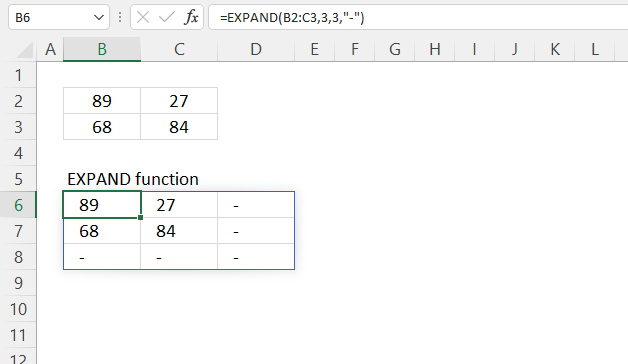
The picture above shows how the EXPAND function increases the original array from two columns and two rows to three columns and three rows. The number of cells increases to 9 cells from 4 cells, 3 rows * 3 columns equals 9 cells. The new cells are padded with a minus sign.
Dynamic array formula in cell B6:
The EXPAND function has 4 arguments. The first argument refers to the source data you want to manipulate. The second argument is the number of rows the new array shall have. The third argument specifies how many columns you want. The fourth and last argument specifies the string you want to pad the new cells with.
The columns and pad_with arguments are optional, however, if you specify the columns argument then you don't need to specify the rows argument if you only need to expand the columns. This means that the rows argument is optional if you specify the columns argument.
4.3.1 Explaining formula
Step 1 - EXPAND function
EXPAND(array, rows, [columns], [pad_with])
Step 2 - Populate arguments
array - B2:C3
rows - 3
[columns] - 3
[pad_with] - "-". The double quotes are needed if a non-numeric value is used.
Step 3 - Evaluate function
EXPAND(B2:C3, 3, 3, "-")
becomes
EXPAND({89, 27;
68, 84}, 3, 3, "-")
and returns
{89, 27, "-";
68, 84, "-";
"-", "-", "-"}
4.4. EXPAND Function example - how to extend an array up and left
The EXPAND function lets you add more rows and columns to an array, they are, however, added to the right and below of the source array. It would be nice if negative values added cells above or the the left of the array. But that won't work, this workaround shows you how to append cells above and to the right of the original array.
Use the following formula to add array containers above and to the left of the original array.
Dynamic array formula in cell B8:
This example demonstrates an array in cell range C3:D4 that we want to expand one row above and one column to the left. As far as I know this is not possible using the EXPAND function, however, the HSTACK and VSTACK lets you add arrays to the original array in a way that makes it possible to expand it above and to the right of the source array.
If you need more than one row and column then use larger empty cell ranges in the HSTACK and VSTACK arguments, this makes it possible to adjust the source array like you want.
Explaining formula
Step 1 - Add arrays horizontally
The HSTACK function lets you combine cell ranges or arrays, it joins data to the first blank cell to the right of a cell range or array (horizontal stacking)
HSTACK(array1, [array2],...)
HSTACK(B3:B4, C3:D4)
becomes
HSTACK({0; 0}, {89, 27; 68, 84})
and returns
{0, 89, 27; 0, 68, 84}.
Step 2 - Add arrays vertically
The VSTACK function lets you combine cell ranges or arrays, it joins data to the first blank cell at the bottom of a cell range or array (vertical stacking).
VSTACK(array1, [array2],...)
VSTACK(B2:D2, HSTACK(B3:B4, C3:D4))
becomes
VSTACK({0, 0, 0}, {0, 89, 27; 0, 68, 84})
and returns
{0, 0, 0;
0, 89, 27;
0, 68, 84}.
4.5. EXPAND Function example - extend array dynamically
The section shows a formula in cell B9 that:
- splits a text string based on a delimiting character. In this case a space character. The output is an array containing each substring in each array value.
- then counts the number of values in the array.
- the count is used to expand the array one row below and one column to the right.
In other words, the formula resizes an array dynamically meaning the array is always one row and one column larger than the source array. Try changing the text value in cell B3 and the dynamic array formula in cell D3 adjusts accordingly.
Dynamic array formula in cell B9:
Explaining formula
You can follow the formula calculations step by step by utilizing the "Evaluate" tool located on the Formula tab on the ribbon.
The new LET function is also possible examining using the "Evaluate" tool, this is not the case with the LAMBDA functions. However, there is no LAMBDA function in this example so no worries yet.
Step 1 - Split text
The TEXTSPLIT function lets you split a string into an array across columns and rows based on delimiting characters.
TEXTSPLIT(Input_Text, col_delimiter, [row_delimiter], [Ignore_Empty])
TEXTSPLIT(B3, " ")
Step 2 - Calculate rows in array and add 1
The ROWS function calculates the number of rows in a given cell range or array.
ROWS(array)
ROWS(TEXTSPLIT(B3, " "))+1
Step 3 - Calculate columns in array and add 1
The COLUMNS function calculates the number of columns in a given cell range or array.
COLUMNS(array)
COLUMNS(TEXTSPLIT(B3, " "))+1
Step 4 - Expand array one row and one column
EXPAND(TEXTSPLIT(B3, " "), ROWS(TEXTSPLIT(B3, " "))+1, COLUMNS(TEXTSPLIT(B3, " "))+1, "-")
becomes
EXPAND({"I", "travel", "the", "world"}, 1+1, 4+1, "-")
and returns
{"I", "travel", "the", "world", "-";
"-", "-", "-", "-", "-"}
Step 5 - Shorten the formula
The LET function lets you name intermediate calculation results which can shorten formulas considerably and improve performance.
LET(name1, name_value1, calculation_or_name2, [name_value2, calculation_or_name3...])
TEXTSPLIT(B3, " ") is repeated three times.
EXPAND(TEXTSPLIT(B3, " "), ROWS(TEXTSPLIT(B3, " "))+1, COLUMNS(TEXTSPLIT(B3, " "))+1, "-")
becomes
LET(x, TEXTSPLIT(B3, " "),EXPAND(x,ROWS(x)+1,COLUMNS(x)+1,"-"))
4.6. EXPAND function error
Can you use negative numbers in the EXPAND function?
No, the EXPAND function returns a #VALUE! error if a negative number is used in the second or third argument. It would have been nice to add rows and columns above and to the right of the array, however, this is not the case. Change the negative numbers in the second and third argument to solve the #VALUE! issue.
Can you use numbers smaller than the actual size of the array in the EXPAND function?
No, numbers smaller than the actual array size also return a #VALUE! error. Cell range B2:D4 has three rows and three columns.
4.7. EXPAND function - values in random order
The image above demonstrates a formula that adds an additional row to cell range B2:D5 and the returns values in random order.
Dynamic array formula in cell B8:
Cell range B2:D5 contains values, the expand function adds another row and pads those cells with a hyphen. The formula in cell B8 returns an array that has the same number of columns as the source range B2:D5 but an additional row. The values are in random order and changes every time you press function key f9.
4.8.1 Explaining formula in cell B8
You can follow the calculations step by step by pressing the "Evaluate" tool located on the Formula tab on the ribbon. This makes it easier to spot errors and understand the formula in greater detail.
Step 1 - Expand array with an extra row
The expand function has four arguments, the first one is the row argument. We want to expand the array by 1 row. The Source data range has four rows, an additional row equals 5 rows.The third argument is the columns argument which does not change, I leave the argument empty. The last argument is the pad_with argument, I use the hyphen character to populate empty cells.
EXPAND(B2:D5,5,,"-")
becomes
EXPAND({89, 27, 26;68, 84, 98;19, 92, 62;37, 63, 45}, 5, , "-")
and returns
{89, 27, 26;
68, 84, 98;
19, 92, 62;
37, 63, 45;
"-", "-", "-"}
Step 2 - Rearrange values into a single column
The TOCOL function rearranges values from a 2D cell range or array to a single column.
TOCOL(array, [ignore], [scan_by_col])
TOCOL(EXPAND(B2:D5,5,,"-"))
becomes
TOCOL({89, 27, 26;
68, 84, 98;
19, 92, 62;
37, 63, 45;
"-", "-", "-"})
and returns
{89; 27; 26; 68; 84; 98; 19; 92; 62; 37; 63; 45; "-"; "-"; "-"}
The semicolon is a row delimiting character, your computer may use an other row delimiting character.
Step 3 - Count cells
The ROWS function returns the number of columns in a given cell range or array.
ROWS(array)
ROWS(TOCOL(EXPAND(B2:D5,5,,"-")))
becomes
ROWS({89; 27; 26; 68; 84; 98; 19; 92; 62; 37; 63; 45; "-"; "-"; "-"})
and returns 15.
Step 4 - Create random cells
The RANDARRAY function returns a table of random numbers across rows and columns.
RANDARRAY([rows], [columns], [min], [max], [whole_number])
RANDARRAY(ROWS(TOCOL(EXPAND(B2:D5, 5, , "-")))))
becomes
RANDARRAY(15)
and returns
{0.215398134613085, 0.390607168196479, ... ,0.83231474462401}.
Step 6 - Rearrange values in random order
The SORTBY function allows you to sort values from a cell range or array based on a corresponding cell range or array.
SORTBY(array, by_array1, [sort_order1], [by_array2, sort_order2],…)
SORTBY(TOCOL(EXPAND(B2:D5, 5, , "-")), RANDARRAY(ROWS(TOCOL(EXPAND(B2:D5, 5, , "-")))))
becomes
SORTBY({89; 27; 26; 68; 84; 98; 19; 92; 62; 37; 63; 45; "-"; "-"; "-"}, {0.215398134613085, 0.390607168196479, ... ,0.83231474462401})
and returns
{"-"; "-"; 84; 62; 89; 92; 98; 37; 63; "-"; 26; 27; 45; 68; 19}.
Step 7 - Rearrange values to the original array size
The WRAPROWS function rearranges values from a single row to a 2D cell range based on a given number of values per row.
WRAPROWS(vector, wrap_count, [pad_with])
WRAPROWS(SORTBY(TOCOL(EXPAND(B2:D5,5,,"-")),RANDARRAY(ROWS(TOCOL(EXPAND(B2:D5,5,,"-"))))),3)
becomes
WRAPROWS({"-"; "-"; 84; 62; 89; 92; 98; 37; 63; "-"; 26; 27; 45; 68; 19},3)
and returns
{84,92,"-";
"-",68,63;
27,37,19;
45,62,"-";
98,89,26}
Step 8 - Shorten formula
The LET function lets you name intermediate calculation results which can shorten formulas considerably and improve performance.
LET(name1, name_value1, calculation_or_name2, [name_value2, calculation_or_name3...])
WRAPROWS(SORTBY(TOCOL(EXPAND(B2:D5,5,,"-")),RANDARRAY(ROWS(TOCOL(EXPAND(B2:D5,5,,"-"))))),3)
becomes
LET(x, TOCOL(EXPAND(B2:D5, 5, , "-")), WRAPROWS(SORTBY(x, RANDARRAY(ROWS(x))), 3))
Useful links
EXPAND function - Microsoft support
Excel EXPAND function to grow array to specified number of rows and columns
EXPAND Function - Exceljet
5. How to use the HSTACK function
What is the HSTACK function?
The HSTACK function lets you combine cell ranges or arrays, it joins data to the first blank cell to the right of a cell range or array
What is HSTACK and abbreviation of?
HSTACK and abbreviation of horizontal stacking.
Which Excel versions have the HSTACK function?
The HSTACK function is available to Excel 365 users and is in the "Array manipulation" category.
Table of Contents
5.1. HSTACK Function Syntax
HSTACK(array1,[array2],...)
Back to top
5.2. HSTACK Function Arguments
array1 | Required. The first cell range or array. |
[array2] | Optional. The second cell range or array to merge. |
5.3. HSTACK Function example
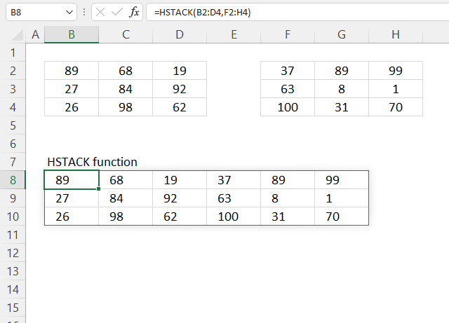
The image above demonstrates how the HSTACK function merges the ranges B2:D4 (blue) and F2:H4 (red). It appends the second cell range (red) to the right of the first cell range (blue).
Formula in cell E4:
Cell range B2:D4 are merged with F2:H4 horizontally. The first array is the leftmost array in the joined array, the remaining arrays are joined in sequence to the right of the first array.
The HSTACK function is great for advanced calculations using the LAMBDA functions, it is there it really shines. The LAMBDA functions let you build recursive formulas that wasn't possible before unless VBA was used.
5.3.1 Explaining formula
Step 1 - HSTACK function
The HSTACK function has one or more arguments, the first argument is required, the subsequent arguments are optional. However, you need at least two arguments to join two cell ranges or arrays.
There is an exception to that if you use parentheses and a comma to differentiate the cell references in the first arguemnt. Here is an example:
=HSTACK((E1:E2,E3:E4))
The formula above joins cell ranges E1:E2 and E3:E4 and both are entered in the first argument. This is however, a very special case but is good to know.
HSTACK(array1,[array2],...)
Step 2 - Populate arguments
array1 - B2:D4
[array2] - F2:H4
Step 3 - Evaluate function
HSTACK(B2:D4, F2:H4)
becomes
HSTACK({89, 68, 19;27, 84, 92;26, 98, 62}, {37, 89, 99;63, 8, 1;100, 31, 70})
and returns
{89, 68, 19, 37, 89, 99;
27, 84, 92, 63, 8, 1;
26, 98, 62, 100, 31, 70}
5.4. HSTACK Function error
The image above demonstrates what happens when you try to append two cell ranges with different numbers of rows. The first cell range (blue) has three columns and the second cell range (red) has 2 columns.
The result is an array containing #N/A errors in locations where no value exists.
Formula in cell E4:
There is a workaround to eliminate errors from the output of the HSTACK function. The IFNA function lets you remove #N/A errors. There is however no argument in the HSTACK function that lets you pad empty cells with a text string.
Formula in cell B8:
The image above shows two different arrays in B2:D4 and F2:H3. The latter array is one row smaller and the HSTACK function pads the empty cells with #N/A! errors.
The HSTACK function in cell B8 replaces all #N/A errors with nothing. Use two double quotes in the second argument to create empty cells. This is demonstrated in cell B8 and cells below and cells to the right.
5.4.1 Explaining formula
Tip! You can follow the formula calculations step by step by using the "Evaluate" tool located on the Formula tab on the ribbon. This makes it easier to spot errors and understand the formula in greater detail.
Step 1 - Stack cell ranges horizontally
HSTACK(B2:D4, F2:H3)
becomes
HSTACK({89, 68, 19;
27, 84, 92;
26, 98, 62},
{37, 89, 99;
63, 8, 1}
)
and returns
{89,68,19,37,89,99;
27,84,92,63,8,1;
26,98,62,#N/A,#N/A,#N/A}
Step 2 - Remove #N/A errors
The IFNA function catches #N/A errors and replaces them with a value you provide.
IFNA(value, value_if_na)
IFNA(HSTACK(B2:D4, F2:G:4), "")
becomes
IFNA(
{89,68,19,37,89,99;
27,84,92,63,8,1;
26,98,62,#N/A,#N/A,#N/A}
, "")
and returns
{89,68,19,37,89,99;
27,84,92,63,8,1;
26,98,62,"","",""}
Note that the IFNA function replaces the #N/A errors with an empty string "".
5.5. Extract unique distinct columns from multiple cell ranges
The image above shows a formula that extracts unique distinct columns from multiple cell ranges.
Formula in cell C10:
Explaining formula
Step 1 - Join cell ranges
HSTACK(array1,[array2],...)
HSTACK(B3:D5, F3:H5)
becomes
HSTACK({89, 27, 26;
"Charles", "Tina", "Linda";
19, 45, 62},
{89, 27, 26;
"Charles", "Tina", "Laura";
24, 45, 62})
and returns
{89,27,26,89,27,26;
"Charles","Tina","Linda","Charles","Tina","Laura";
19,45,62,24,45,62}.
Bolded values are two duplicate columns.
Step 2 - Extract unique distinct columns
The UNIQUE function is a new Excel 365 function that returns unique and unique distinct values/rows.
UNIQUE(array, [by_col], [exactly_once])
UNIQUE(HSTACK(B3:D5, F3:H5), TRUE)
becomes
UNIQUE({89,27,26,89,27,26;
"Charles","Tina","Linda","Charles","Tina","Laura";
19,45,62,24,45,62}, TRUE)
and returns
{89,27,26,89,26;
"Charles","Tina","Linda","Charles","Laura";
19,45,62,24,62}
Useful resources
HSTACK function - Microsoft support
How to combine ranges / arrays in Excel with VSTACK & HSTACK functions
6. How to use the TAKE function
What is the TAKE function?
The TAKE function returns a given number of rows or columns from a 2D cell range or array filtering the remaining rows out.
The TAKE function is available to Excel 365 users and is in the "Array manipulation" category.
Table of Contents
- TAKE Function Syntax
- TAKE Function Arguments
- TAKE Function example
- TAKE Function example - return columns
- TAKE Function example - return columns and rows
- TAKE Function example - negative values
- TAKE Function alternative
- TAKE Function - values in random order
- TAKE Function - multiple source ranges
- Get Excel *.xlsx file
6.1. TAKE Function Syntax
TAKE(array, rows, [columns])
Back to top
6.2. TAKE Function Arguments
The TAKE function has three arguments, the first and second argument are required and the third is optional.
array | Required. The source cell range or array. |
rows | Required. The number of contiguous rows to return, a negative number returns contiguous rows from the end. |
[columns] | Optional. The number of contiguous columns to return, a negative number returns contiguous rows from the end. |
6.3. TAKE Function example
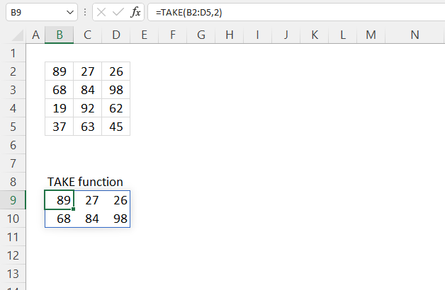
The picture above shows how the TAKE function returns the two first rows from cell range B2:D5.
Dynamic array formula in cell B9:
The source range is B2:D5 and the second argument is 2. This means that row 1 and row 2 counting from the top is returned to the output array, however, row 3 and 4 are deleted. The TAKE function is useful for resizing arrays, this makes it easier to work with specific rows or columns. For example, you want to know the median number from columns 1 and 2. The TAKE function is very useful for this kind of scenario.
6.3.1 Explaining formula
You can follow the calculations step by step by pressing the "Evaluate" tool located on the Formula tab on the ribbon. This makes it easier to spot errors and understand the formula in greater detail.
Step 1 - TAKE function
The TAKE function has three arguments, the first two are required. This example needs only the first two arguments.
TAKE(array, rows, [columns])
Step 2 - Populate arguments
The first argument is the array or cell range which is B2:D5. The sond argument is rows and is 2 in this example.
array - B2:D5
rows - 2
[columns] -
Step 3 - Evaluate function
The following lines show how the TAKE function keeps the first two rows and deletes the remaining rows.
TAKE(B2:D5, 2)
becomes
TAKE({89, 27, 26;68, 84, 98;19, 92, 62;37, 63, 45}, 2)
and returns
{89, 27, 26;
68, 84, 98}
6.4. TAKE Function example - return columns
The image above demonstrates how to return specific columns using the TAKE function. Cell range B2:D5 contains values, it has four rows and three columns. This example shows how to keep the two first columns and leave the remaining columns out.
Formula in cell B6:
Note that the second argument is not required if you supply a number for the third argument. The function works perfectly as long as you type a number in at least one of argument rows or columns.
6.5. TAKE Function example - return rows and columns
The image above demonstrates how to return both rows and columns using the TAKE function. Note that it only returns the intersection of the chosen rows and columns, see the image below.
The intersection are those values that are in both column 1 and 2, and also in rows 1 and 2. The blue rectangles shown in the image above shows both groups, the red rectangle shows the intersection of those two groups.
Formula in cell B9:
TAKE(array, rows, [columns])
This example shows that you can use both the second rows argument and the third columns argument at the same time. Remember that the output is the intersection and not the union.
6.6. TAKE Function example - negative values
The TAKE function lets you use negative arguments, this means that the function returns rows/columns from the end. The TAKE function counts columns from left to right and rows from top to bottom.
Formula in cell B9:
However, negative values forces the TAKE function to count the rows from bottom up to the top and the columns from right to the left.
TAKE(array, rows, [columns])
The image above shows that the rows argument is -2 and that takes the two last rows from cell range B2:D5. The columns argument is -2 as well and that takes the two last columns. Only the intersection of these groups are returned to cell B9. The red rectangle in the image above shows the intersection.
6.7. TAKE function alternative
It is possible to return the two first rows using the OFFSET function, however, the OFFSET function is volatile and may slow down your worksheet if you use many of them. Volatile means that the OFFSET function recalculates more often than regular Excel functions.
Array formula in cell B9:
This array formula should work in most Excel versions. I recommend using the TAKE function in Excel 365, it is not volatile.
6.7.1 How to enter an array formula
Earlier Excel versions require you to enter array formulas in a specific way in order to show all values in the array. The following steps shows how to enter an array formula in earlier Excel versions. Excel 365 does not have this disadvantage, you can enter all formulas as a regular function in Excel 365.
- Double press with left mouse button on with the left mouse button on cell B9, a prompt appears.
- Type or copy/paste the formula to cell B9.
- Press and hold CTRL + SHIFT simultaneously.
- Press Enter once.
- Release all keys.
The formula now has leading and trailing curly brackets, don't enter these characters yourself. They appear automatically.
6.7.2 Explaining formula in cell B6
Step 1 - OFFSET function
The OFFSET function returns a reference to a range that is a given number of rows and columns from a given reference.
OFFSET(reference, rows, columns, [height], [width])
Step 2 - Populate arguments
The OFFSET function has five arguments, three are required and two are optional. The rows and columns arguments are not required in this example because we specify the height and width arguments in this example.
reference - B2:D5
rows -Â
columns -Â
[height] - 2
[width] - 3
Step 3 - Evaluate OFFSET function
OFFSET(B2:D5,,,2,3)
becomes
OFFSET({89, 27, 26;68, 84, 98;19, 92, 62;37, 63, 45},,,2,3)
and returns
{89, 27, 26; 68, 84, 98}.
6.8. TAKE function - values in random order
The image above shows a formula that returns values in random order from the two first rows in a given 2D cell range. Cell range B2:D5 contains some random values, it has three columns and four rows.
Dynamic array formula in cell B8:
The formula extracts the two first rows and then returns those values in random order, the returned array has the same size as the two first rows in the source data range.
The formula in cell B8 spills values below and to the right of cell B8 as far as needed. A #SPILL! error is displayed if any of the destination cells are not empty. Delete the nonempty cells and the error goes away.
6.8.1 Explaining formula in cell B8
Tip! You can follow the formula calculations step by step by using the "Evaluate" tool located on the Formula tab on the ribbon. This makes it easier to spot errors and understand the formula in greater detail.
Step 1 - Extract two first rows
The first argument is B2:D5 and the second argument rows is 2.
TAKE(B2:D5, 2)
becomes
TAKE({89, 27, 26;68, 84, 98;19, 92, 62;37, 63, 45}, 2)
and returns
{89, 27, 26;68, 84, 98}.
This filters the two first rows and leaves the remaining rows out.
Step 2 - Rearrange values to a single row
The TOROW function rearranges values from a 2D cell range or array to a single row.
TOROW(array, [ignore], [scan_by_col])
TOROW(TAKE(B2:D5,2))
becomes
TOROW({89, 27, 26;68, 84, 98})
and returns
{89, 27, 26, 68, 84, 98}.
Step 3 - Count cells
The COLUMNS function returns the number of columns in a given cell range or array.
COLUMNS(array)
COLUMNS(TOROW(TAKE(B2:D5,2)))
becomes
COLUMNS({89, 27, 26, 68, 84, 98})
and returns 6.
Step 4 - Count rows
The ROWS function returns the number of rows in a given cell range or array.
ROWS (array)
ROWS(TAKE(B2:D5,2))
becomes
ROWS({89, 27, 26; 68, 84, 98})
and returns 2.
Step 5 - Create random decimal numbers
The RANDARRAY function returns a table of random numbers across rows and columns.
RANDARRAY([rows], [columns], [min], [max], [whole_number])
RANDARRAY(,COLUMNS(TOROW(TAKE(B2:D5,2))))
becomes
RANDARRAY(,6)
and returns
{0.215398134613085, 0.390607168196479, ... ,0.83231474462401}.
Step 6 - Rearrange values in random order
The SORTBY function allows you to sort values from a cell range or array based on a corresponding cell range or array.
SORTBY(array, by_array1, [sort_order1], [by_array2, sort_order2],…)
SORTBY(TOROW(TAKE(B2:D5,2)),RANDARRAY(,COLUMNS(TAKE(B2:D5,2))))
becomes
SORTBY({89, 27, 26, 68, 84, 98}, {0.215398134613085, 0.390607168196479, ... ,0.83231474462401})
and returns
{84, 89, 26, 27, 98, 68}.
Step 7 - Rearrange values to original array size
The WRAPCOLS function rearranges values from a single row to a 2D cell range based on a given number of values per column.
WRAPCOLS(vector, wrap_count, [pad_with])
WRAPCOLS(SORTBY(TOROW(TAKE(B2:D5,2)),RANDARRAY(,COLUMNS(TOROW(TAKE(B2:D5,2))))),ROWS(TAKE(B2:D5,2)))
becomes
WRAPCOLS({84, 89, 26, 27, 98, 68},ROWS(TAKE(B2:D5,2)))
becomes
WRAPCOLS({84, 89, 26, 27, 98, 68}, 2)
and returns
{84, 89, 26; 27, 98, 68}
Step 8 - Shorten formula
The LET function lets you name intermediate calculation results which can shorten formulas considerably and improve performance.
LET(name1, name_value1, calculation_or_name2, [name_value2, calculation_or_name3...])
WRAPCOLS(SORTBY(TOROW(TAKE(B2:D5,2)),RANDARRAY(,COLUMNS(TOROW(TAKE(B2:D5,2))))),TOROW(TAKE(B2:D5,2)))
becomes
LET(z,TAKE(B2:D5,2),x,TOROW(z),WRAPCOLS(SORTBY(x,RANDARRAY(,COLUMNS(x))),ROWS(z)))
6.9. TAKE Function - multiple source ranges
The picture above shows a formula that merges three non-contiguous cell ranges and return values from the two first columns. The three non-contiguous cell ranges are B3:D6, F3:H6, and J3:L6. These cell ranges are merged vertically meaning the first cell range B3:D6 is at the top, the second cell range F3:H6 is joined below B3:D6. The third cell range J3:L6 is merged below F3:H6, together they form a larger array containing three columns and 12 rows.
Dynamic array formula in cell B9:
The TAKE function extracts the first two columns (Item and Quantity) and filters out the third (Price). The output is displayed in cell B9 and cells below and to the right as far as needed. This is a Excel 365 formula and is entered as a regular formula. A #SPILL error is shown if at least one of the destinations cells are not empty.
This technique is useful if data sets are located on different worksheets and you need to perform specific calculations to give columns. For example, the average of each items quantity or the median price etc.
6.9.1 Explaining formula
Tip! You can follow the formula calculations step by step by using the "Evaluate" tool located on the Formula tab on the ribbon. This makes it easier to spot errors and understand the formula in greater detail.
Step 1 - Stack values horizontally
The VSTACK function lets you combine cell ranges or arrays, it joins data to the first blank cell at the bottom of a cell range or array (vertical stacking)
VSTACK(array1, [array2],...)
VSTACK(B3:D6, F3:H6, J3:L6)
becomes
VSTACK({"Peach", 43, 1.03;"Blueberry", 39, 1.48;"Apple", 46, 1.1;"Grapefruit", 14, 0.72}, {"Mandarin", 29, 0.78;"Raspberry", 33, 1.07;"Plum", 25, 0.9;"Mango", 37, 1.13}, {"Pear", 17, 0.63;"Orange", 31, 1.06;"Lime", 17, 1.27;"Kiwi", 45, 0.58})
and returns
{"Peach", 43, 1.03;
"Blueberry", 39, 1.48;
"Apple", 46, 1.1;
"Grapefruit", 14, 0.72;
"Mandarin", 29, 0.78;
"Raspberry", 33, 1.07;
"Plum", 25, 0.9;
"Mango", 37, 1.13;
"Pear", 17, 0.63;
"Orange", 31, 1.06;
"Lime", 17, 1.27;
"Kiwi", 45, 0.58}
Step 2 - Wrap values to rows
TAKE(VSTACK(B3:D6, F3:H6, J3:L6), , 2)
becomes
TAKE({"Peach", 43, 1.03;
"Blueberry", 39, 1.48;
"Apple", 46, 1.1;
"Grapefruit", 14, 0.72;
"Mandarin", 29, 0.78;
"Raspberry", 33, 1.07;
"Plum", 25, 0.9;
"Mango", 37, 1.13;
"Pear", 17, 0.63;
"Orange", 31, 1.06;
"Lime", 17, 1.27;
"Kiwi", 45, 0.58}, , 2)
and returns
{"Peach", 43;
"Blueberry", 39;
"Apple", 46;
"Grapefruit", 14;
"Mandarin", 29;
"Raspberry", 33;
"Plum", 25;
"Mango", 37;
"Pear", 17;
"Orange", 31;
"Lime", 17;
"Kiwi", 45}
Useful resources
TAKE function - Microsoft support
Excel TAKE function to extract rows or columns from array
7. How to use the TOCOL function
What is the TOCOL function?
The TOCOL function lets you rearrange values in 2D cell ranges to a single column.
TOCOL stands for to column.
Which Excel version is TOCOL in?
The TOCOL function is available to Excel 365 users
What category is the TOCOL function in?
The TOCOL function is in the "Array manipulation" category.
Table of Contents
- TOCOL Function Syntax
- TOCOL Function Arguments
- TOCOL Function example
- TOCOL Function example - by column
- TOCOL Function - blanks and errors
- TOCOL Function alternative
- TOCOL Function - multiple cell ranges as source
- Extract unique distinct values from a cell range
- Extract unique distinct values from multiple cell ranges
- Get Excel *.xlsx file
7.1. TOCOL Function Syntax
The TOCOL function has three arguments, the first one is required the other two are optional.
TOCOL(array, [ignore], [scan_by_col])
7.2. TOCOL Function Arguments
array | Required. The source cell range or array. Use parentheses and comma delimiter to add more arrays or cell ranges. See section 7 below for an example. |
[ignore] | Optional. Ignore specified values. 0 - keep all values (default) 1 - ignore blanks 2 - ignore errors 3- ignore blanks and errors |
[scan_by_col] | Optional. How the function fetches the values from the source. FALSE - by row (default). TRUE - by column. |
7.3. TOCOL Function example
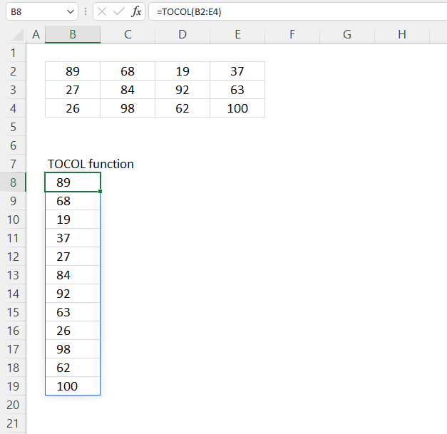
The image above demonstrates how the TOCOL function rearranges the values to fit a single column, and that it is fetching values by row in its default state.
This means that the TOCOL function takes the values in cell B2:E4 row by row and transposes them so they fit a single column. For example, the first row is 89, 68, 19, and 37 and they are distributed horizontally in B2:E2,
The TOCOL function rearranges the values so they are distributed vertically like this: 89; 68; 19; 37. It the goes on to the second row and transposes those values below the first row. The blue arrows shows this beahviour in the TOCOL functions default state. You can however change this so it scans the cell range column by column instead of row by row.
Dynamic array formula in cell E4:
The TOCOL function is incredibly useful if you want to for example extract unique distinct values across multiple columns. The UNIQUE function requires an array containing values distributed vertically one by one. If not the UNIQUE function extracts unique distinct rows.
7.3.1 Explaining formula
Tip! You can follow the formula calculations step by step by using the "Evaluate" tool located on the Formula tab on the ribbon. This makes it easier to spot errors and understand the formula in greater detail. The following steps shows the calculations in great detail.
Step 1 - TOCOL function
TOCOL(array, [ignore], [scan_by_col])
Step 2 - Populate arguments
array - B2:E4
Step 3 - Evaluate function
TOCOL(B2:E4)
becomes
TOCOL({89, 68, 19, 37;
27, 84, 92, 63;
26, 98, 62, 100})
and returns
{89; 68; 19; 37; 27; 84; 92; 63; 26; 98; 62; 100}
7.4. TOCOL Function example - by column
The image above demonstrates how the TOCOL function rearranges the values to fit a single column. This example shows it fetching values column by column. Default value is FALSE - which means by row.
The blue arrows show that the TOCOL function is also capable of rearranging values column by column. The first column is 89, 27, 26, 68 which is also displayed in the output array in cell E4. The second column is then put below these values, this continues column by column until all columns have been scanned.
Dynamic array formula in cell E4:
The third argument lets you specify the scan state: scan_by_col or scan_by_row. TRUE means scan_by_col and FALSE means scan_by_row which is also the default state.
7.4.1 Explaining formula
Tip! You can follow the formula calculations step by step by using the "Evaluate" tool located on the Formula tab on the ribbon. This makes it easier to spot errors and understand the formula in greater detail. The following steps shows the calculations in great detail.
Step 1 - TOCOL function
TOCOL(array, [ignore], [scan_by_col])
Step 2 - Populate arguments
array - B2:E4
[scan_by_col]) - TRUE
Step 3 - Evaluate function
TOCOL(B2:E4, , TRUE)
becomes
TOCOL({89, 68, 19, 37;
27, 84, 92, 63;
26, 98, 62, 100})
and returns
{89; 68; 19; 37; 27; 84; 92; 63; 26; 98; 62; 100}
7.5. TOCOL Function - blanks and errors
The TOCOL function can handle blanks and errors, however, you must specify that in the aruments if you want that functionality. The image above demonstrates what happens when your source data has empty values and errors. The result is an array containing a 0 (zero) located at the empty values and the error values are kept.
Dynamic array formula in cell E4:
The image below shows how to deal with blanks and error values.
You can ignore blank and error values using the second argument.
Here are all valid numbers for the second argument:
0 - keep all values (default)
1 - ignore blanks
2 - ignore errors
3- ignore blanks and errors
Dynamic array formula in cell E4:
There is an instance when this doesn't work. This happens if you use the IF function to filter specific values in the TOCOL function. Here is an example.
=TOCOL(IF(B2:E4<50,"",B2:E4), 3)
The TOCOL function can't handle blanks and errors from the IF function at all, they all show even if you use 3 in the second argument. This is kind of a disappointment, I hope Microsoft software engineers fix this issue in upcoming releases.
7.5.1 Explaining formula
TOCOL(array, [ignore], [scan_by_col])
TOCOL(B2:E4, 3)
becomes
TOCOL({89, 68, 19, 37;
27, 0, 92, 63;
26, 98, 62, #DIV/0!}
)
and returns
{89; 68; 19; 37; 27; 92; 63; 26; 98; 62}
7.6. TOCOL alternative
There are no great alternative formulas for earlier Excel versions. Here are a few links:
- Rearrange values in a cell range to a single column
- Combine cell ranges ignore blank cells
- Merge two columnsÂ
- Merge three columns into one list
7.7. TOCOL function - multiple cell ranges as source
You can consolidate values across worksheets if you combine the VSTACK function and the TOCOL function, the formula spills values into a single column.
The image above shows how to combine values from cell ranges B2:C3, E2:F3, and h3:I3 into a single column.
Dynamic array formula in cell B8:
The formula in cell B8 joins the three non-adjacent cell ranges vertically and then scans the resulting array row by row and rearranges the values to a single column. You can try different outcomes based on how you want the values arranged. The HSTACK function joins the cell ranges horizontally, and the third argument in the TOCOL function lets you specify how the function scans and rearranges the values in the array. The options are scan_by_row or scan_by_column.
Update! The TOCOL function accepts multiple references in the array argument. There is no need for the VSTACK function. Here is how:
The parentheses and a delimiting comma let you use multiple non-adjacent cell ranges. Note that this is done in the first argument.
7.7.1 Explaining formula
Tip! You can follow the formula calculations step by step by using the "Evaluate" tool located on the Formula tab on the ribbon. This makes it easier to spot errors and understand the formula in greater detail. The following steps shows the calculations in great detail.
Step 1 - Stack values from multiple sources
The VSTACK function lets you combine cell ranges or arrays, it joins data to the first blank cell at the bottom of a cell range or array.
VSTACK(array1,[array2],...)
VSTACK(B2:C3, E2:F3, h3:I3)
becomes
VSTACK({89,68;27,84}, {19,37;92,63}, {26,98;62,100})
and returns
{89,68;
27,84;
19,37;
92,63;
26,98;
62,100}
Step 2 - Rearrange values into one column
TOCOL(VSTACK(B2:C3, E2:F3, h3:I3))
becomes
TOCOL({89,68;
27,84;
19,37;
92,63;
26,98;
62,100})
and returns
{89; 68; 27; 84; 19; 37; 92; 63; 26; 98; 62; 100}
7.8. Extract unique distinct values from a multi-column cell range
The UNIQUE function doesn't let you extract unique distinct values if your source data has multiple columns, it will return unique distinct rows instead.
However, the TOCOL function allows you to rearrange the values to a single column array, and that lets you extract unique distinct values.
Dynamic array formula in cell B8:
The TOCOL function makes it so much easier to extract unique distinct values. The values must be arranged in a single column for the UNIQUE function to work properly.
7.8.1 Explaining formula
Tip! You can follow the formula calculations step by step by using the "Evaluate" tool located on the Formula tab on the ribbon. This makes it easier to spot errors and understand the formula in greater detail. The following steps shows the calculations in great detail.
Step 1 - Rearrange values
TOCOL(array, [ignore], [scan_by_col])
TOCOL(B2:G5)
returns {"Elizabeth"; "Patricia"; ... ; "Mary"}.
The column delimiting character changed from a comma to a semicolon in the array above. This means that each value is in a new row, in other words, values are rearranged to fit a single column.
Step 2 - Extract unique distinct values
The UNIQUE function is a new Excel 365 function that returns unique and unique distinct values/rows.
UNIQUE(array,[by_col],[exactly_once])
UNIQUE(TOCOL(B2:G5))
returns {"Elizabeth";"Patricia";"Jennifer";"William";"John";"Robert";"Mary";"Michael";"Linda"}.
7.9. Extract unique distinct values from multiple cell ranges
You can consolidate values across worksheets, rearrange values so they fit a single column, and then extract unique distinct values.
The image above shows a formula that extracts unique distinct values from three different non-adjacent cell ranges.
Dynamic array formula in cell B8:
Update!
No need to use the HSTACK function. Use the comma as a union operator, it combines multiple cell ranges.
This formula is useful for getting values across worksheets consolidated into one array, it is also dynamic meaning it changes instantly if the source ranges change.
7.9.1 Explaining formula
Step 1 - Rearrange values
The HSTACK function lets you combine cell ranges or arrays, it joins data to the first blank cell to the right of a cell range or array (horizontal stacking)
HSTACK(array1,[array2],...)
HSTACK(B2:C5, E2:F5, h3:I5)
returns {"Elizabeth", "Patricia", ... , "Mary"}
Step 2 - Rearrange values to one column
TOCOL(array, [ignore], [scan_by_col])
TOCOL(HSTACK(B2:C5, E2:F5, h3:I5))
returns
{"Elizabeth"; "Patricia"; ... ; "Mary"}.
Step 3 - Extract unique distinct values
The UNIQUE function is a new Excel 365 function that returns unique and unique distinct values/rows.
UNIQUE(array,[by_col],[exactly_once])
UNIQUE(TOCOL(HSTACK(B2:C5, E2:F5, h3:I5)))
returns
{"Elizabeth"; "Patricia"; "Jennifer"; "William"; "John"; "Robert"; "Mary"; "Michael"; "Linda"}.
Useful resources
TOCOL function - Microsoft support
Excel TOCOL function - convert range to single column
8. How to use the TOROW function
What is the TOROW function?
The TOROW function rearranges values from a 2D cell range to a single row.
Dynamic array formula in cell B8:
What Excel version has the TOROW function?
The TOROW function is available to Excel 365 subscribers.
What category is the TOROW function?
The TOROW functionis in the "Array manipulation" category.
How do I enter an Excel 365 dynamic array formula?
A dynamic array formula is entered as a regular formula, however, it spills array values automatically to adjacent cells below or to the right or both.
Table of Contents
8.1. TOROW Function Syntax
The TOROW function has three arguments, the first one array is required, the remaining two ignore and scan_by_col is optional.
TOROW(array, [ignore], [scan_by_col])
8.2. TOROW Function Arguments
array | Required. The source cell range or array. |
[ignore] | Optional. Ignore specified values. 0 - keep all values (default) 1 - ignore blanks 2 - ignore errors 3- ignore blanks and errors |
[scan_by_col] | Optional. How the function fetches the values from the source. FALSE - by row (default). TRUE - by column. |
8.3. TOROW Function example
The graphic above shows how the TOROW function rearranges values to fit a single row; in its default form, it obtains values by row. This means that it gets the values from the first row then the second row and so on until all rows have been scanned and processed.
Dynamic array formula in cell B8:
The TOROW function is useful for resizing an array to a single row. It is an Excel 365 function and spills values to the cell below and to the cells to the right. A #SPILL! error shows up if the destination cells are not empty. Make sure you delete old values to make it work properly.
8.3.1 Explaining formula
Tip! You can follow the formula calculations step by step by using the "Evaluate" tool located on the Formula tab on the ribbon. This makes it easier to spot errors and understand the formula in greater detail. The following steps shows the calculations in great detail.
Step 1 - TOROW function
TOROW(array, [ignore], [scan_by_col])
Step 2 - Populate arguments
array - B2:E4
Step 3 - Evaluate function
TOROW(B2:E4)
becomes
TOROW({89, 68, 19, 37;
27, 84, 92, 63;
26, 98, 62, 45})
and returns
{89; 68; 19; 37; 27; 84; 92; 63; 26; 98; 62; 45}
8.4. TOROW Function example - by column
The picture above demonstrates how the TOROW function rearranges the values to fit a single row, this example shows it fetching values column by column. Default value is FALSE which means by row.
Dynamic array formula in cell B8:
This example shows in great detail how the TOROW function scans the source array by column and then returns the output to single row.
8.4.1 Explaining formula
Step 1 - TOROW function
TOROW(array, [ignore], [scan_by_col])
Step 2 - Populate arguments
array - B2:E4
[scan_by_col]) - TRUE
Step 3 - Evaluate function
TOROW(B2:E4, , TRUE)
becomes
TOROW({89, 68, 19, 37;
27, 84, 92, 63;
26, 98, 62, 100})
and returns
{89, 27, 26, 68, 84, 98, 19, 92, 62, 37, 63, 45}
The comma is a column delimiting character, the semicolon is a row delimiting character. You may have other delimiting characters, it depends on your regional settings.
Which delimiting values do I use?
- Double press with left mouse button on an empty cell.
- Type = (equal sign).
- Select a cell range containing two rows and two columns. They can be empty, it doesn't matter.
- Press F9 to convert the cell reference to constants.
- The array that appears shows your delimiting characters.
8.5. TOROW Function - blanks and errors
The image above demonstrates what happens when your source data has empty values and errors.
The result is a horizontal array containing a 0 (zero) instead of empty values, and the error values are not ignored but kept.
Dynamic array formula in cell B8:
The picture above shows how to handle blanks and error values. The second argument lets you determine the outcome for blank and error values.
Here are all valid numbers for the second argument:
0 - keep all values (default)
1 - ignore blanks
2 - ignore errors
3- ignore blanks and errors
Dynamic array formula in cell B8:
8.5.1 Explaining formula
TOROW(array, [ignore], [scan_by_col])
TOROW(B2:E4, 3)
becomes
TOROW({89, "", 19, 37;
27, 0, 92, 63;
26, 98, 62, #N/A}
)
and returns
{89, 19, 37, 27, 84, 92, 63, 26, 98, 62}
8.6. TOROW function alternative
The following formula rearranges values so they fit a single column, however, the formula doesn't return an array of values. It extracts each value one by one using relative cell references.
You need to copy the cell and paste as far as needed to the right. This formula works in most Excel versions, I recommend the TOROW function if you are a Excel 365 subscriber.
Formula in cell B7:
This formula shows how much effort is needed to resize an array to a single row in earlier Excel versions. The TOROW function shows progress is being made in Excel.
8.6.1 Explaining formula
Tip! You can follow the formula calculations step by step by using the "Evaluate" tool located on the Formula tab on the ribbon. This makes it easier to spot errors and understand the formula in greater detail. The following steps shows the calculations in great detail.
Step 1 - Calculate the number of columns in a given cell range
The COLUMNS function returns the number of columns in a given cell range.
COLUMNS(array)
COLUMNS($B$2:$E$4)
returns 4.
Step 2 - Calculate column number of relative cell reference
The COLUMN function returns the column number of the top-left cell of a cell reference.
COLUMN(reference)
COLUMN(A1)-1
becomes
1-1 equals 0 (zero)
Step 3 - Calculate row number
The QUOTIENT function returns the integer portion of a division.
QUOTIENT(numerator, denominator)
QUOTIENT(COLUMN(A1)-1, COLUMNS($B$2:$E$4))+1
becomes
QUOTIENT(0, 4)+1
becomes
0+1 equals 1.
Step 4 - Calculate column number
The MOD function returns the remainder after a number is divided by a divisor.
MOD(number, divisor)
MOD(COLUMN(A1)-1, COLUMNS($B$2:$E$4))+1
becomes
MOD(0, 4)+1
becomes
0 + 1 equals 1.
Step 5 - Get value
The INDEX function returns a value from a cell range, you specify which value based on a row and column number.
INDEX(array, [row_num], [column_num], [area_num])
INDEX($B$2:$E$4, QUOTIENT(COLUMN(A1)-1, COLUMNS($B$2:$E$4))+1, MOD(COLUMN(A1)-1, COLUMNS($B$2:$E$4))+1)
becomes
INDEX($B$2:$E$4, 1, 1)
and returns 89 in cell B7.
8.7. TOROW function - values in random order
The image above shows a formula that returns values to a single row in random order. Cell range B2:E4 contains values, this is our source data range. The formula below rearranges the values to a single row and then changes their positions randomly.
Dynamic array formula in cell B8:
This formula is useful for randomizing values and resizing their source array. It works only in Excel 365 and spills values to the right as far as needed. A#SPILL error is displayed if the destination cells are not empty.
Explaining formula in cell B8
Tip! You can follow the formula calculations step by step by using the "Evaluate" tool located on the Formula tab on the ribbon. This makes it easier to spot errors and understand the formula in greater detail. The following steps shows the calculations in great detail.
Step 1 - Calculate the number of rows in cell ref
The ROWS function returns the number of rows in a given cell range.
ROWS(array)
ROWS(B2:E4)
returns 3. There are three rows in cell range B2:E4.
Step 2 - Calculate the number of columns in cell ref
The COLUMNS function returns the number of columns in a given cell range.
COLUMNS(array)
COLUMNS(B2:E4)
returns 4. There are four columns in cell range B2:E4.
Step 3 - Calculate the number of cells in cell ref
The asterisk lets you multiply numbers in an Excel formula. This useful now that we want to calculate the total number of cells in B2:E4.
ROWS(B2:E4)*COLUMNS(B2:E4)
becomes
3*4 equals 12.
Step 4 - Create random values
The RANDARRAY function returns a table of random numbers across rows and columns.
RANDARRAY([rows], [columns], [min], [max], [whole_number])
RANDARRAY(, ROWS(B2:E4)*COLUMNS(B2:E4))
becomes
RANDARRAY(, 12)
and returns 12 random decimal values:
{0.464680665246457, 0.768212043461448, ... ,0.281771048521311}
Step 5 - Rearrange values
TOROW(B2:E4)
returns
{"A", "B", "C", "D", "E", "F", "G", "H", "I", "J", "K", "L"}.
Step 6 - Sort values in random order
The SORTBY function allows you to sort values from a cell range or array based on a corresponding cell range or array.
SORTBY(array, by_array1, [sort_order1], [by_array2, sort_order2],…)
SORTBY(TOROW(B2:E4), RANDARRAY(, ROWS(B2:E4)*COLUMNS(B2:E4)))
becomes
SORTBY({"A", "B", "C", "D", "E", "F", "G", "H", "I", "J", "K", "L"}, {0.464680665246457, 0.768212043461448, ... ,0.281771048521311})
and returns
{"H", "E", "I", "F", "L", "B", "D", "A", "J", "K", "G", "C"}. Press F9 to recalcualte values, this creates a new random order.
Useful resources
TOROW function - Microsoft support
Excel TOROW function - Myonlinetraininghub
9. How to use the VSTACK function
The VSTACK function lets you combine cell ranges or arrays, it joins data to the first blank cell at the bottom of a cell range or array. The VSTACK function is available to Excel 365 users and is in the "Array manipulation" category.
What is VSTACK an abbreviation of?Â
VSTACK stands for vertical stacking meaning arrays are arranged on top of each other.
What is an array?
An array is an array of values meaning multiple values in its simplest form. Excel functions may accept an array as the input value or argument.
Some Excel functions return an array of values instead of a single value. Excel 365 handles these arrays automatically whereas previous versions need to be entered as an array formula. For example, the FREQUENCY function returns multiple values.
You can also create a formula that returns multiple values, in Excel 365 they are named dynamic array formulas and in earlier versions named array formulas. The most simple dynamic array formula I know is this: = A1:A2, it returns two values populated in cells A1 and A2.
Table of Contents
9.1. VSTACK Function Syntax
The VSTACK function has one required arument and the remaining aruments are optional.
VSTACK(array1,[array2],...)
9.2. VSTACK Function Arguments
array1 | Required. The first cell range or array. |
[array2] | Optional. The second cell range or array to merge. |
9.3. VSTACK Function example
The image above demonstrates how the VSTACK function merges the ranges B2:D4 (blue) and F2:H4 (red). It appends the second cell range (red) to the bottom of the first cell range (blue).
Formula in cell E4:
The VSTACK function is great for consolidating data from multiple worksheets, it is easy to use. Keep in mind to not reference the table headers or you will get table headers from each cell reference in the returning array. Check out formulas that use VSTACK function.
9.3.1 Explaining formula
Tip! You can follow the formula calculations step by step by using the "Evaluate" tool located on the Formula tab on the ribbon. This makes it easier to spot errors and understand the formula in greater detail. The following steps shows the calculations in great detail.
Step 1 - VSTACK function
VSTACK(array1,[array2],...)
Step 2 - Populate arguments
array1 - B2:D4
[array2] - F2:H:4
Step 3 - Evaluate function
VSTACK(B2:D4, F2:H:4)
returns
{89, 68, ... , 70}
9.4. VSTACK Function errors
The image above demonstrates what happens when you try to append two cell ranges containing a different number of columns. The first cell range (blue) has three columns and the second cell range (red) has 2 columns.
The result is an array containing #N/A errors in locations where no value exists.
Formula in cell E4:
The IFNA function lets you remove #N/A errors.
Formula in cell B8:
The array in cell B8 is now empty of #N/A! errors, see the image above.
9.4.1 Explaining formula
Step 1 - Stack cell ranges vertically
VSTACK(B2:D4, F2:G:4)
returns {89, 68, ... , #N/A}
Step 2 - Remove #N/A errors
IFNA(VSTACK(B2:D4, F2:G:4), "")
returns {89, 68, ... , 31, ""}
9.5. VSTACK Function alternative
There is unfortunately no way to merge cell ranges in earlier Excel versions unless you are willing to manually merge the ranges or use a User Defined Function.
The image above shows how to manually merge two cell ranges, this technique works in all Excel versions as far as I know, however, you are required to enter the array as an array formula in order to show all values.
Here are the steps:
- Select cell range B8:D:13. The resulting array is three columns wide and contains six rows, make sure you select a cell range that fits your data.
- Type = (equal sign).
- Select with mouse the first cell range B2:D4.
- Type a + (plus sign).
- Select with mouse the second cell range F2:H4.
- Select F2:H4 in the formula.
- Press F9 to convert the cell range to constants.
- Repeat steps 6 and 7 using the first cell range B2:D4, the result looks like this:
- Select the last curly bracket of the first array, the plus sign and the first curly bracket of the second array:
- Press Delete to remove those characters.
- Type a semicolon ;
- Steps 12 to 14 show how to enter the array as an array formula.
Press and hold CTRL + SHIFT simultaneously. - Press Enter once.
- Release all keys.
The formula has now a leading and ending curly bracket, they appear automatically. Don't enter these characters yourself.
This article describes how to merge cell ranges using a User Defined Function: Combine cell ranges ignore blank cells (User Defined Function)
9.6. Extract unique distinct rows from multiple cell ranges
This example demonstrates how to extract unique distinct rows/records from multiple non-adjacent cell ranges. The image above shows one data set in B3:D5 and another in F3:H5.
The VSTACK function stacks these data sets on top of each other. The UNIQUE function the merges duplicate rows/records to one distinct row/record for each instance.
Formula in cell B9:
This formula is an Excel 365 dynamic array formula. It is entered as regular formula and it spills values to cells below and to the right of B9 as far as needed. A #SPILL! error is shown if the destination cells are not empty.
Explaining formula
Tip! You can follow the formula calculations step by step by using the "Evaluate" tool located on the Formula tab on the ribbon. This makes it easier to spot errors and understand the formula in greater detail. The following steps shows the calculations in great detail.
Step 1 - Join cell ranges
VSTACK(array1,[array2],...)
VSTACK(B3:D5, F3:H5)
returns {89, "Charles",... , 62}.
Step 2 - Extract unique distinct rows
The UNIQUE function is a new Excel 365 function that returns unique and unique distinct values/rows.
UNIQUE(array,[by_col],[exactly_once])
UNIQUE(VSTACK(B3:D5, F3:H5), FALSE, FALSE)
returns
{89, "Charles", ... , 62}
The bolded rows are duplicates, only one instance of those rows in the result.
9.7. VSTACK Function works with 3D ranges
The image above demonstrates how to use 3D ranges in the VSTACK function. You must have data in the same location on each worksheet for this to work.
What is a 3d range?
A 3d range is a cell reference that references multiple worksheets in only one cell reference. However, you need to know how to create a 3D reference which is easy and the data must be on the same cell range on each worksheet. The image above shows that data on worksheet 1, 2 and 3 are on the same location.
Dynamic array formula in cell B3:
Some of the data sets are smaller than others, this makes the formula get blank values as well from cell ranges that contain blanks. The FILTER function filters out blanks based on if each cell in column A in each sheet is empty.
9.7.1 How to enter the 3D range cell reference
This is entered as a regular formula, however, the 3D range needs to be explained in greater detail.
To create this reference: '1:3'!A2:C10 follow these steps:
- Double press with left mouse button on cell B3, the prompt appears.
- Type: =FILTER(VSTACK(
- Go to worksheet: 1
- Select cell range A2:C10
- Press and hold SHIFT key.
- Select the remaining worksheets, they are 2 and 3 in this example.
- Type the remaining part of the formula and repeat the above steps for the second 3D range.
- Press Enter.
9.7.2 Explaining formula
Tip! You can follow the formula calculations step by step by using the "Evaluate" tool located on the Formula tab on the ribbon. This makes it easier to spot errors and understand the formula in greater detail. The following steps shows the calculations in great detail.
Step 1 - Merge data from three diffrent worksheets vertically
VSTACK('1:3'!A2:C10)
becomes
VSTACK('1'!A2:C10,'2'!A2:C10,'3'!A2:C10)
returns
{89,"Charles",..., 0}
Step 2 - Remove empty rows
The FILTER function filters values based on a condition or criteria.
FILTER(array, include, [if_empty])
FILTER(VSTACK('1:3'!A2:C10),VSTACK('1:3'!A2:A10)<>"")
returns
{89,"Charles",...,34}
Useful resources
VSTACK function - Microsoft support
How to combine ranges / arrays in Excel with VSTACK & HSTACK functions
10. How to use the WRAPCOLS function
What is the WRAPCOLS function?
The WRAPCOLS function rearranges values from a single row to a 2D cell range based on a given number of values per column.
The WRAPCOLS function is available to Excel 365 users
Which category contains the WRAPCOLS function?
The WRAPCOLS function is in the "Array manipulation" category.
Table of Contents
10.1. WRAPCOLS Function Syntax
WRAPCOLS(vector, wrap_count, [pad_with])
10.2. WRAPCOLS Function Arguments
vector | Required. The source cell range or array. |
wrap_count | Required. The number of values per column, the last row may be smaller. |
[pad_with] | Optional. Value to pad with if there is an insufficient number of values in the last row. The default value is #N/A! |
10.3. WRAPCOLS Function example
The picture above shows how the WRAPCOLS function rearranges values in a row to create a 2D range based on the number of values per column specified in the second argument: wrap_count.
Dynamic array formula in cell B8:
The source range is B2:M2 and contains 12 values. The formula in cell B8 creates an array based on 4 values per column, this returns an array containing 4 rows and 3 columns.
For example, the output array is 4 rows and 4 columns if the source range contains 15 values. The size of the array is determined by the number of cells in the source range the wrap_count number.
10.3.1 Explaining formula
Tip! You can follow the formula calculations step by step by using the "Evaluate" tool located on the Formula tab on the ribbon. This makes it easier to spot errors and understand the formula in greater detail. The following steps shows the calculations in great detail.
Step 1 - WRAPCOLS function
WRAPCOLS(vector, wrap_count, [pad_with])
Step 2 - Populate arguments
vector - B2:M2
wrap_count - 4
Step 3 - Evaluate function
WRAPCOLS(B2:M2, 4)
becomes
WRAPCOLS({89, 68, 19, 37, 27, 84, 92, 63, 26, 98, 62, 45})
and returns
{89, 27, 26;
68, 84, 98;
19, 92, 62;
37, 63, 45}.
10.4. WRAPCOLS Function example - pad with
The WARPACOLS function builds an array based on the number of cells in the source range and the number specified in the wrap_cols argument. This may produce more values than the source range contains.
The WRAPCOLS function returns #N/A errors in empty containers in its default state. The #N/A errors may show up in empty cells on the last column, use the [pad_with] argument to populate empty cells and get rid of the #N/A error.
The following formula populates an array containing some empty cells, however, empty cells are padded with "A" in this example. This is not the case with the formula shown in the image above. Cells D8 and D9 contain #N/A errors.
Formula in cell B6:
The image below demonstrates how to populate empty cells with the text string "A".
10.5. WRAPCOLS function alternative
The image above shows a formula that works in earlier Excel versions. This formula wraps the values in cell range B2:K2 to fit four values per row. Change the bolded number in the formula below to adjust the number of columns.
Formula in cell B6:
Change bolded numbers to the number of rows you want in the 2D range.
10.5.1 Explaining formula in cell B6
Tip! You can follow the formula calculations step by step by using the "Evaluate" tool located on the Formula tab on the ribbon. This makes it easier to spot errors and understand the formula in greater detail. The following steps shows the calculations in great detail.
Step 1 - Calculate the number of columns in a given cell range
The COLUMN function returns the column number of the top-left cell of a cell reference.
COLUMN(reference)
COLUMN(A1) - 1
becomes
1-1 equals 0 (zero).
Step 2 - Calculate column number of relative cell reference
The ROW function returns the row number of a cell reference.
ROW(reference)
ROW(A1)
returns 1.
Step 3 - Multiply
The asterisk lets you multiply numbers in an Excel formula.
The parentheses control the order of calculation, we want to subtract before we multiply.
(COLUMN(A1)-1)*4
becomes
0*4 equals 0 (zero).
Step 4 - Calculate column number
The INDEX function returns a value from a cell range, you specify which value based on a row and column number.
INDEX(array, [row_num], [column_num], [area_num])
INDEX($B$2:$K$2,,ROW(A1)+(COLUMN(A1)-1)*4)
becomes
INDEX($B$2:$K$2,,1)
and returns 89 in cell B6.
Step 5 - Return #N/A for row numbers above condition
The IF function returns one value if the logical test is TRUE and another value if the logical test is FALSE.
IF(logical_test, [value_if_true], [value_if_false])
IF(ROW(A1)>4,NA(),INDEX($B$2:$K$2,,ROW(A1)+(COLUMN(A1)-1)*4))
becomes
IF(ROW(A1)>4,NA(),89)
becomes
IF(FALSE, NA(), 89)
and returns 89.
10.6. WRAPCOLS function - values in random order
The image above demonstrates a formula that rearranges values in random order with four columns. The formula gets the values from B2:M2 and puts them in random order. Then the formula reshapes the array to 4 rows and as many columns as needed.
Dynamic array formula in cell B6:
This formula is great for putting given values in random order and to a given array size. The formula returns a new order every time the worksheet recalculates or Function key F9 is pressed.
The formula returns a #SPILL! error if the destination cells contain at least one value. Remove the value and the formula is able to display all values.
10.6.1 Explaining formula in cell B8
Tip! You can follow the formula calculations step by step by using the "Evaluate" tool located on the Formula tab on the ribbon. This makes it easier to spot errors and understand the formula in greater detail. The following steps shows the calculations in great detail.
Step 1 - Calculate the number of cells in cell ref
The COLUMNS function returns the number of columns in a given cell range.
COLUMNS(array)
COLUMNS(B2:M2)
returns 12.
Step 2 - Create random decimal values
The RANDARRAY function returns a table of random numbers across rows and columns.
RANDARRAY([rows], [columns], [min], [max], [whole_number])
RANDARRAY(, COLUMNS(B2:M2))
becomes
RANDARRAY(, 12)
and returns
{0.732441255476154, 0.953587479053817, ... , 0.0191675082920368}
Step 3 - Sort values based on random decimals
The SORTBY function allows you to sort values from a cell range or array based on a corresponding cell range or array.
SORTBY(array, by_array1, [sort_order1], [by_array2, sort_order2],…)
SORTBY(B2:M2, RANDARRAY(, COLUMNS(B2:M2)))
becomes
SORTBY(B2:M2, {0.732441255476154, 0.953587479053817, ... , 0.0191675082920368})
becomes
SORTBY({89, 68, 19, 37, 27, 84, 92, 63, 26, 98, 62, 45}, {0.732441255476154, 0.953587479053817, ... , 0.0191675082920368})
and returns
{98, 68, 45;27, 19, 26;62, 92, 89;84, 37, 63}.
Step 5 - Wrap values
WRAPCOLS(SORTBY(B2:M2, RANDARRAY(, COLUMNS(B2:M2))), 4)
becomes
WRAPCOLS({98, 68, 45;27, 19, 26;62, 92, 89;84, 37, 63}, 4)
and returns
{98, 68, 45;
27, 19, 26;
62, 92, 89;
84, 37, 63}
Press F9 to recalculate values, this creates a new random order.
10.7. WRAPCOLS Function - multiple source ranges
The picture above shows a formula that joins values from multiple non-adjacent source ranges and then rearranges the array to a 2D range based on given rows. In this case 4 rows per column.
Dynamic array formula in cell B6:
This formula makes it really easy to consolidate data from multiple worksheets and show them in an array with given number of rows per column.
The image shows three non-adjacent cell ranges B2:M2, B4:G4, and B6:K6. The output array is shown in cell B6, the Excel 365 dynamic array formula spills values to cells below and to the right as far as needed,
10.7.1 Explaining formula
Step 1 - Stack values horizontally
The HSTACK function lets you combine cell ranges or arrays, it joins data to the first blank cell to the right of a cell range or array (horizontal stacking)
HSTACK(array1, [array2],...)
HSTACK(B2:M2, B4:G4, B6:K6)
becomes
HSTACK({89, 68, 19, 37, 27, 84, 92, 63, 26, 98, 62, 45}, {49, 65, 30, 59, 10, 10}, {52, 30, 55, 58, 33, 58, 31, 93, 27, 97})
and returns
{89, 68, 19, 37, 27, 84, 92, 63, 26, 98, 62, 45, 49, 65, 30, 59, 10, 10, 52, 30, 55, 58, 33, 58, 31, 93, 27, 97}.
Step 2 - Wrap values to rows
WRAPCOLS(HSTACK(B2:M2, B4:G4, B6:K6), 4)
becomes
WRAPCOLS({89, 68, 19, 37, 27, 84, 92, 63, 26, 98, 62, 45, 49, 65, 30, 59, 10, 10, 52, 30, 55, 58, 33, 58, 31, 93, 27, 97}, 4)
and returns
{89, 27, 26, 49, 10, 55, 31;
68, 84, 98, 65, 10, 58, 93;
19, 92, 62, 30, 52, 33, 27;
37, 63, 45, 59, 30, 58, 97}
Useful resources
How to Use the WRAPCOLS Function in Excel
WRAPCOLS function - Microsoft support
11. How to use the WRAPROWS function
What is the WRAPROWS function?
The WRAPROWS function rearranges values from a single row to a 2D cell range.
The WRAPROWS function is available to Excel 365 users and is in the "Array manipulation" category.
Table of Contents
11.1. WRAPROWS Function Syntax
The WRAPROWS function has two required aruments and one optional.
WRAPROWS(vector, wrap_count, [pad_with])
11.2. WRAPROWS Function Arguments
vector | Required. The source cell range or array. |
wrap_count | Required. The number of values per row, the last row may be smaller. |
[pad_with] | Optional. Value to pad with if there is an insufficient number of values in the last row. The default value is #N/A! |
11.3. WRAPROWS Function example
The picture above shows how the WRAPROWS function rearranges values to fit the requirement specified in the second argument: wrap_count. Cell range B2:M2 contains values distributed horizontally.
Dynamic array formula in cell B8:
The WRAPROWS function resizes the the array B2:M2 and returns an array containing 4 columns per row. This means that the number of rows changes and the number of columns is constant. In other words , a cell reference to a larger cell range returns 4 columns per row, however, the number of rows are more.
The Excel 365 dynamic array formula spills values to cell B8 and to cells below and to the right as far as needed. Excel returns a #SPILL! error if the destination cells contain other values, in other words, the destination cells must be empty.
11.3.1 Explaining formula
Tip! You can follow the formula calculations step by step by using the "Evaluate" tool located on the Formula tab on the ribbon. This makes it easier to spot errors and understand the formula in greater detail. The following steps shows the calculations in great detail.
Step 1 - WRAPROWS function
WRAPROWS(vector, wrap_count, [pad_with])
Step 2 - Populate arguments
vector - B2:E4
wrap_count - 4
Step 3 - Evaluate function
WRAPROWS(B2:M2, 4)
becomes
WRAPROWS({89, 68, 19, 37, 27, 84, 92, 63, 26, 98, 62, 45})
and returns
{89, 68, 19, 37; 27, 84, 92, 63; 26, 98, 62, 45}.
11.4. WRAPROWS Function example - pad with
The image above shows the WRAPROWS function in cell B6, the output array has #N/A errors in empty cells on the last row. Use the [pad_with] argument to populate empty cells, which is the third argument in the WRAPROWS function.
Formula in cell B6:
The formula above does not populate empty cells, it returns #N/A in those cells. The image below demonstrates how to populate empty cells with the text string "A".
The third argument contains "A" which means that the WRAPROWS function pads empty cells with the string "A".
Formula in cell B6:
It is possible to populate empty cells with nothing as well. Two double quotes "" returns blanks in the empty cells.
11.5. WRAPROWS function alternative
This formula is for earlier Excel versions without the WRAPCOLS function. The formula wraps the values in cell range B2:K2 to fit four columns per row. Change the bolded number in the formula below to adjust the number of columns.
Formula in cell B6:
The image above shows values in cell range B2:M2. The formula in cell B6 rearranges the values using the INDEX, COLUMN and ROW functions which are available in earlier Excel versions. The formula is a regular formula, however, you need to copy cell B6 and paste it to cells to the right as far as needed. The copy thos cells and paste to cells below as far as needed. This is required to do in order for the relative cell references to work properly.
11.5.1 Explaining formula in cell B6
Tip! You can follow the formula calculations step by step by using the "Evaluate" tool located on the Formula tab on the ribbon. This makes it easier to spot errors and understand the formula in greater detail. The following steps shows the calculations in great detail.
Step 1 - Calculate the number of columns in a given cell range
The COLUMN function returns the column number of the top-left cell of a cell reference.
COLUMN(reference)
COLUMN(A1) returns 1.
Step 2 - Calculate column number of relative cell reference
The ROW function returns the row number of a cell reference.
ROW(reference)
ROW(A1)-1
becomes
1 - 1 equals 0 (zero).
Step 3 - Multiply
The asterisk lets you multiply numbers in an Excel formula.
The parentheses controls the order of calculation, we want to subtract before we multiply.
(ROW(A1)-1)*4
becomes
0*4 equals 0 (zero)
Step 4 - Calculate column number
The INDEX function returns a value from a cell range, you specify which value based on a row and column number.
INDEX(array, [row_num], [column_num], [area_num])
INDEX($B$2:$K$2,,COLUMN(A1)+(ROW(A1)-1)*4)
becomes
INDEX($B$2:$K$2,,1)
and returns 89 in cell B6.
11.6. WRAPROWS function - values in random order
The image above shows a formula in cell B6 that rearranges values in random order and the output array has four columns per row. It is an Excel 365 formula and spills values to cells to the right and below as far as needed. The source data range is B2:M2 and the output array changes the order of the values every time you press F9 or the worksheets recalculates.
Dynamic array formula in cell B6:
The formula returns a #SPILL! error if a values is in at least one of the destination cells. Remove the value and the #SPILL! error disappears.
11.6.1 Explaining formula in cell B8
Tip! You can follow the formula calculations step by step by using the "Evaluate" tool located on the Formula tab on the ribbon. This makes it easier to spot errors and understand the formula in greater detail. The following steps shows the calculations in great detail.
Step 1 - Calculate the number of cells in cell ref
The COLUMNS function returns the number of columns in a given cell range.
COLUMNS(array)
COLUMNS(B2:M2)
returns 12.
Step 2 - Create random decimal values
The RANDARRAY function returns a table of random numbers across rows and columns.
RANDARRAY([rows], [columns], [min], [max], [whole_number])
RANDARRAY(, COLUMNS(B2:M2))
becomes
RANDARRAY(, 12)
and returns
{0.732441255476154, 0.953587479053817, ... , 0.0191675082920368}
Step 3 - Sort values based on random decimals
The SORTBY function allows you to sort values from a cell range or array based on a corresponding cell range or array.
SORTBY(array, by_array1, [sort_order1], [by_array2, sort_order2],…)
SORTBY(B2:M2, RANDARRAY(, COLUMNS(B2:M2)))
becomes
SORTBY(B2:M2, {0.732441255476154, 0.953587479053817, ... , 0.0191675082920368})
and returns
Step 4 - Create random values
The RANDARRAY function returns a table of random numbers across rows and columns.
RANDARRAY([rows], [columns], [min], [max], [whole_number])
RANDARRAY(, ROWS(B2:E4)*COLUMNS(B2:E4))
becomes
RANDARRAY(, 12)
and returns 12 random decimal values:
{0.464680665246457, 0.768212043461448, ... ,0.281771048521311}
Step 6 - Sort values in random order
The SORTBY function allows you to sort values from a cell range or array based on a corresponding cell range or array.
SORTBY(array, by_array1, [sort_order1], [by_array2, sort_order2],…)
SORTBY(B2:M2, RANDARRAY(, COLUMNS(B2:M2)))
becomes
SORTBY(B2:M2, {0.732441255476154, 0.953587479053817, ... , 0.0191675082920368})
becomes
SORTBY({89, 68, 19, 37, 27, 84, 92, 63, 26, 98, 62, 45}, {0.732441255476154, 0.953587479053817, ... , 0.0191675082920368})
{63, 45, 27, 68, 84, 26, 92, 62, 98, 37, 89, 19}
Step 5 - Wrap values
WRAPROWS(SORTBY(B2:M2, RANDARRAY(, COLUMNS(B2:M2))), 4)
becomes
WRAPROWS({63, 45, 27, 68, 84, 26, 92, 62, 98, 37, 89, 19}, 4)
and returns
{63,45,27,68;
84,26,92,62;
98,37,89,19}
Press F9 to recalculate values, this creates a new random order.
11.7. WRAPROWS Function - multiple source ranges
The graphic above demonstrates a formula that merges values from cell ranges B2:M2, B4:G4, and B6:K6, then wraps the values to a 2D array. The size of the array is four columns per row and the number of rows depends on the number of cells in the source ranges B2:M2, B4:G4, and B6:K6.
Dynamic array formula in cell B6:
This formula is an Excel 365 formula and is entered as a regular formula. The formula spills values to cells below and to the right as far as needed. The formula returns a #SPILL! error if at least one of the destination cells are occupied with other values. They need to be empty, delete the values and the #SPILL error disappears.
11.7.1 Explaining formula
Tip! You can follow the formula calculations step by step by using the "Evaluate" tool located on the Formula tab on the ribbon. This makes it easier to spot errors and understand the formula in greater detail. The following steps shows the calculations in great detail.
Step 1 - Stack values horizontally
The HSTACK function lets you combine cell ranges or arrays, it joins data to the first blank cell to the right of a cell range or array (horizontal stacking)
HSTACK(array1, [array2],...)
HSTACK(B2:M2, B4:G4, B6:K6)
becomes
HSTACK({89, 68, 19, 37, 27, 84, 92, 63, 26, 98, 62, 45}, {49, 65, 30, 59, 10, 10}, {52, 30, 55, 58, 33, 58, 31, 93, 27, 97})
and returns
{89, 68, 19, 37, 27, 84, 92, 63, 26, 98, 62, 45, 49, 65, 30, 59, 10, 10, 52, 30, 55, 58, 33, 58, 31, 93, 27, 97}.
Step 2 - Wrap values to rows
WRAPROWS(HSTACK(B2:M2, B4:G4, B6:K6), 4)
becomes
WRAPROWS({89, 68, 19, 37, 27, 84, 92, 63, 26, 98, 62, 45, 49, 65, 30, 59, 10, 10, 52, 30, 55, 58, 33, 58, 31, 93, 27, 97}, 4)
and returns
{89, 68, 19, 37;
27, 84, 92, 63;
26, 98, 62, 45;
49, 65, 30, 59;
10, 10, 52, 30;
55, 58, 33, 58;
31, 93, 27, 97}
Useful resources
WRAPCOLS function - Microsoft support
Convert column / row to range in Excel: WRAPCOLS & WRAPROWS functions
Excel categories
Leave a Reply
How to comment
How to add a formula to your comment
<code>Insert your formula here.</code>
Convert less than and larger than signs
Use html character entities instead of less than and larger than signs.
< becomes < and > becomes >
How to add VBA code to your comment
[vb 1="vbnet" language=","]
Put your VBA code here.
[/vb]
How to add a picture to your comment:
Upload picture to postimage.org or imgur
Paste image link to your comment.
Contact Oscar
You can contact me through this contact form